Author Contributions
Conceptualization, D.L., B.K., T.P. and J.-W.Y.; Methodology, D.L. and J.-W.Y.; Software, D.L.; Validation, D.L., B.K., T.P., J.-W.Y. and H.P.; Investigation, D.L. and H.P.; Writing—Original Draft, D.L. and H.P.; Writing—Review and Editing, J.-W.Y. and H.P.; Supervision, B.K., T.P., J.-W.Y. and H.P.; Funding Acquisition, T.P. All authors have read and agreed to the published version of the manuscript.
Figure 1.
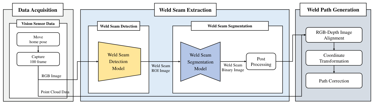
Proposed framework consisting of three subcomponents: data acquisition, weld seam extraction, and weld path generation.
Figure 1.
Proposed framework consisting of three subcomponents: data acquisition, weld seam extraction, and weld path generation.
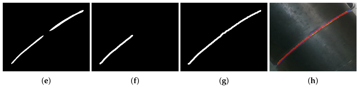
Figure 2.
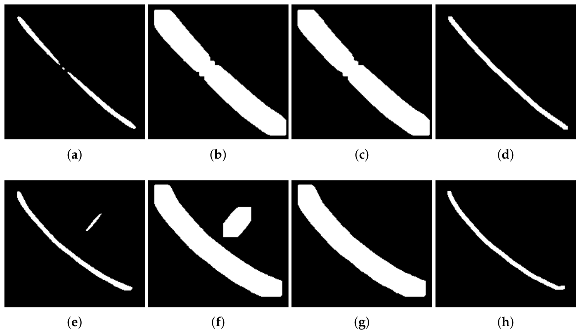
Image post-processing pipeline applied to weld seam mask images. (a,e) Segmentation outputs from the deep learning model; (b,f) after morphological dilation to enhance discontinuous weld regions; (c,g) after max contour filtering to remove noise; and (d,h) final results after thinning to extract centerlines for weld path generation.
Figure 2.
Image post-processing pipeline applied to weld seam mask images. (a,e) Segmentation outputs from the deep learning model; (b,f) after morphological dilation to enhance discontinuous weld regions; (c,g) after max contour filtering to remove noise; and (d,h) final results after thinning to extract centerlines for weld path generation.
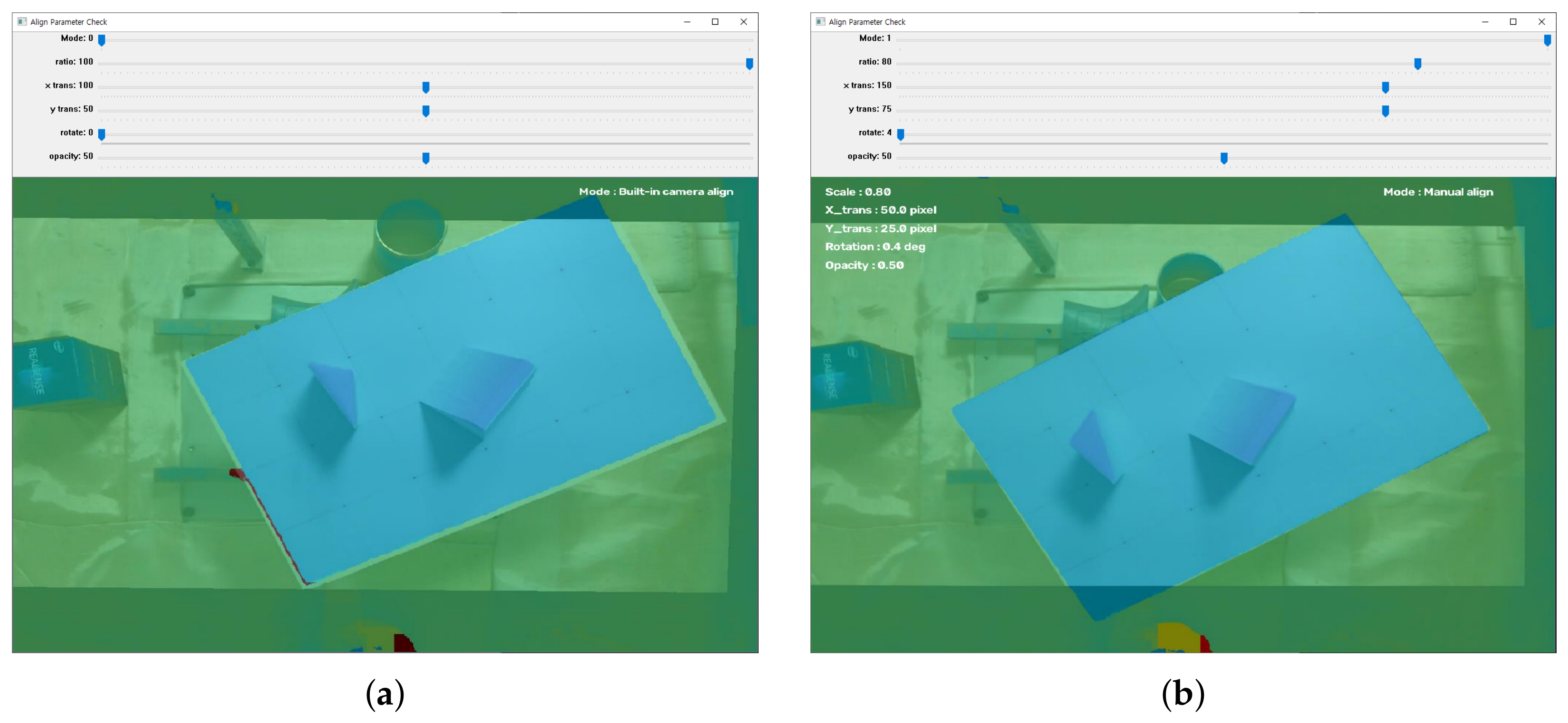
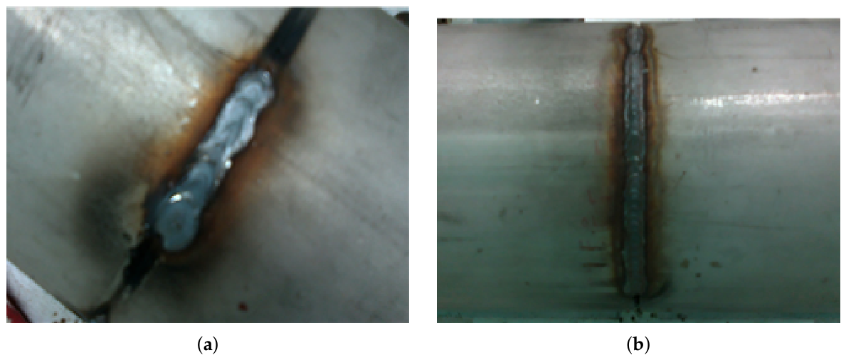
Figure 3.
Comparison of RGB–D image alignment using the built-in camera alignment and the proposed manual alignment tool. (a) The result obtained using the built-in camera alignment provided by the RGB-D sensor; (b) the manually adjusted alignment achieved by tuning the scale, translation, rotation, and opacity parameters.
Figure 3.
Comparison of RGB–D image alignment using the built-in camera alignment and the proposed manual alignment tool. (a) The result obtained using the built-in camera alignment provided by the RGB-D sensor; (b) the manually adjusted alignment achieved by tuning the scale, translation, rotation, and opacity parameters.
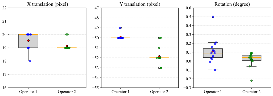
Figure 4.
Distribution of the manually selected RGB-to-depth registration parameters obtained by two independent operators over 15 repeated calibration trials. The boxplots present the distributions of the X translation, Y translation, and rotation parameters.
Figure 4.
Distribution of the manually selected RGB-to-depth registration parameters obtained by two independent operators over 15 repeated calibration trials. The boxplots present the distributions of the X translation, Y translation, and rotation parameters.
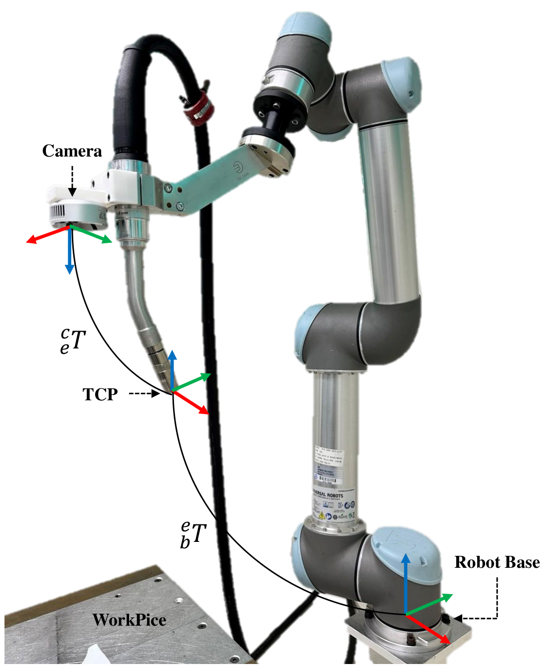
Figure 5.
Coordinate frame transformations between the robot base, end-effector, and camera coordinate frames.
Figure 5.
Coordinate frame transformations between the robot base, end-effector, and camera coordinate frames.
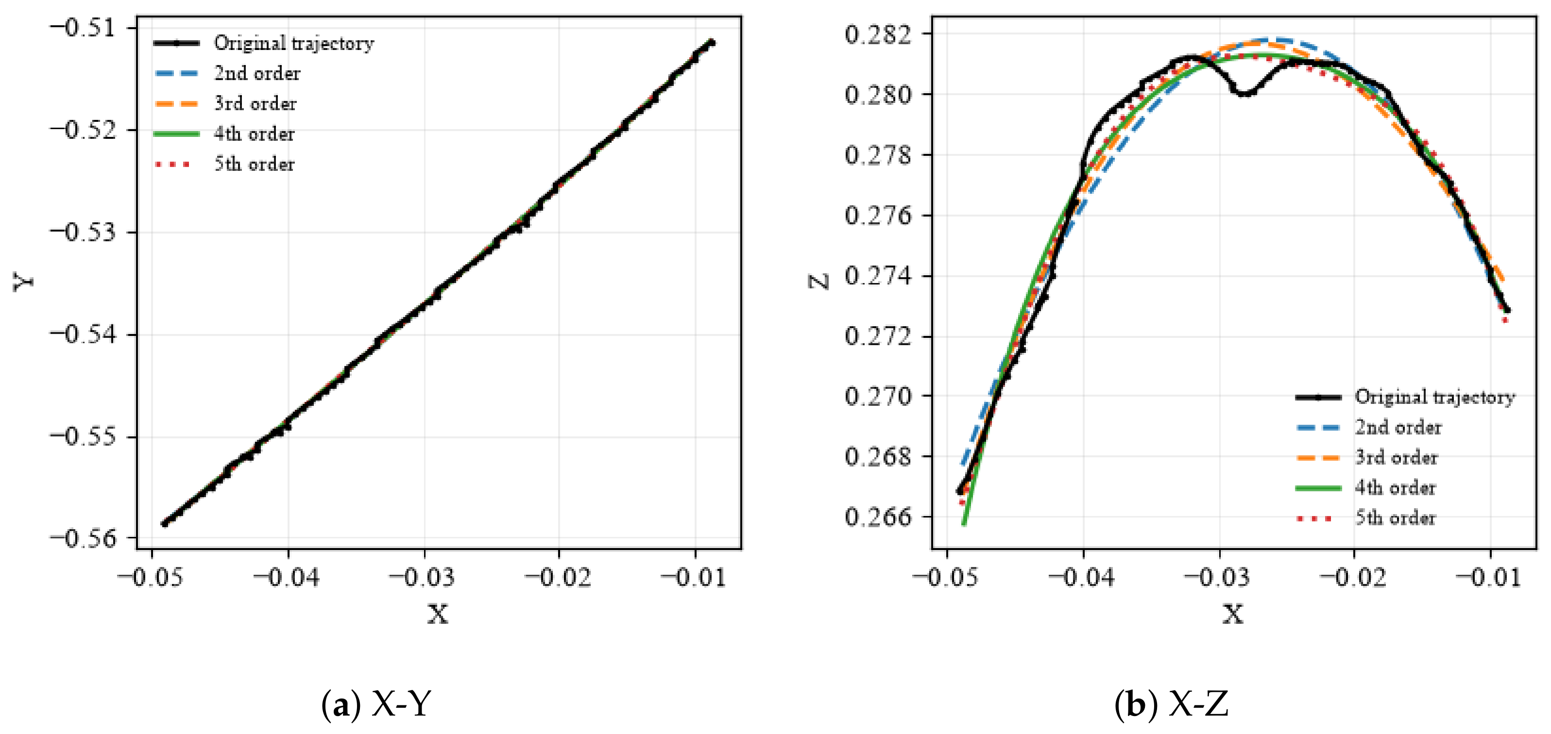
Figure 6.
Comparison of polynomial fitting results with different polynomial orders for the generated robotic welding path. (a) Fitting results on the X–Y plane. (b) Fitting results on the X–Z plane. The black solid line denotes the original trajectory, and the colored curves represent the trajectories obtained using second-, third-, fourth-, and fifth-order polynomial fitting.
Figure 6.
Comparison of polynomial fitting results with different polynomial orders for the generated robotic welding path. (a) Fitting results on the X–Y plane. (b) Fitting results on the X–Z plane. The black solid line denotes the original trajectory, and the colored curves represent the trajectories obtained using second-, third-, fourth-, and fifth-order polynomial fitting.
Figure 7.
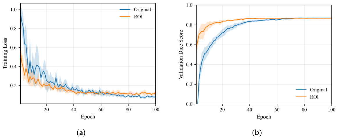
Training convergence of the U-Net segmentation model across five independent random seed experiments. (a) Training loss and (b) validation Dice score. Solid lines and shaded regions represent the mean and one standard deviation, respectively.
Figure 7.
Training convergence of the U-Net segmentation model across five independent random seed experiments. (a) Training loss and (b) validation Dice score. Solid lines and shaded regions represent the mean and one standard deviation, respectively.
Figure 8.
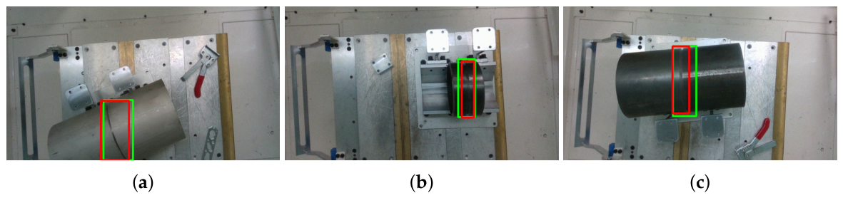
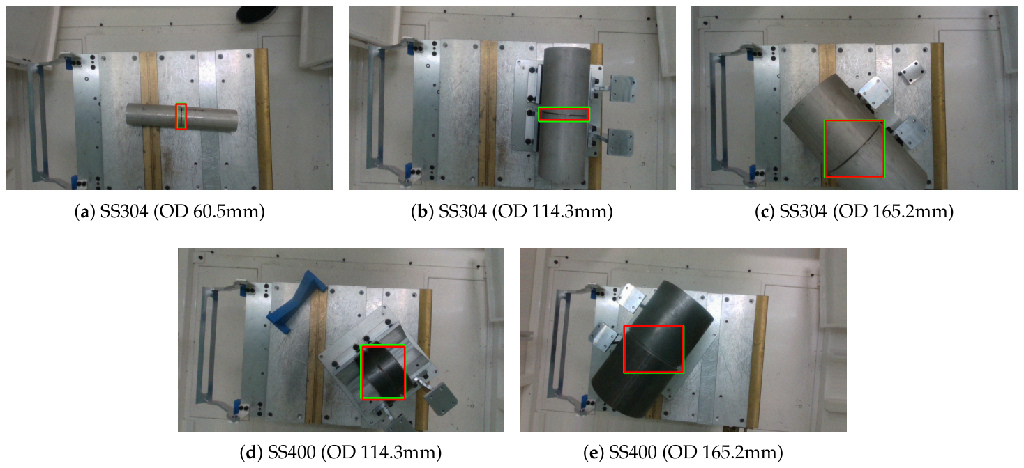
Representative successful weld seam detection results for five different pipe types. (a–e) Successful detection results for each pipe type. The red and green bounding boxes represent the predicted ROI and ground-truth annotation, respectively.
Figure 8.
Representative successful weld seam detection results for five different pipe types. (a–e) Successful detection results for each pipe type. The red and green bounding boxes represent the predicted ROI and ground-truth annotation, respectively.
Figure 9.
Representative ROI detection error cases showing minor localization differences between the predicted bounding boxes and the ground-truth bounding boxes. (a–c) Three representative examples of ROI detection results exhibiting slight localization differences. The red and green bounding boxes represent the predicted ROI and ground-truth annotation, respectively.
Figure 9.
Representative ROI detection error cases showing minor localization differences between the predicted bounding boxes and the ground-truth bounding boxes. (a–c) Three representative examples of ROI detection results exhibiting slight localization differences. The red and green bounding boxes represent the predicted ROI and ground-truth annotation, respectively.
Figure 10.
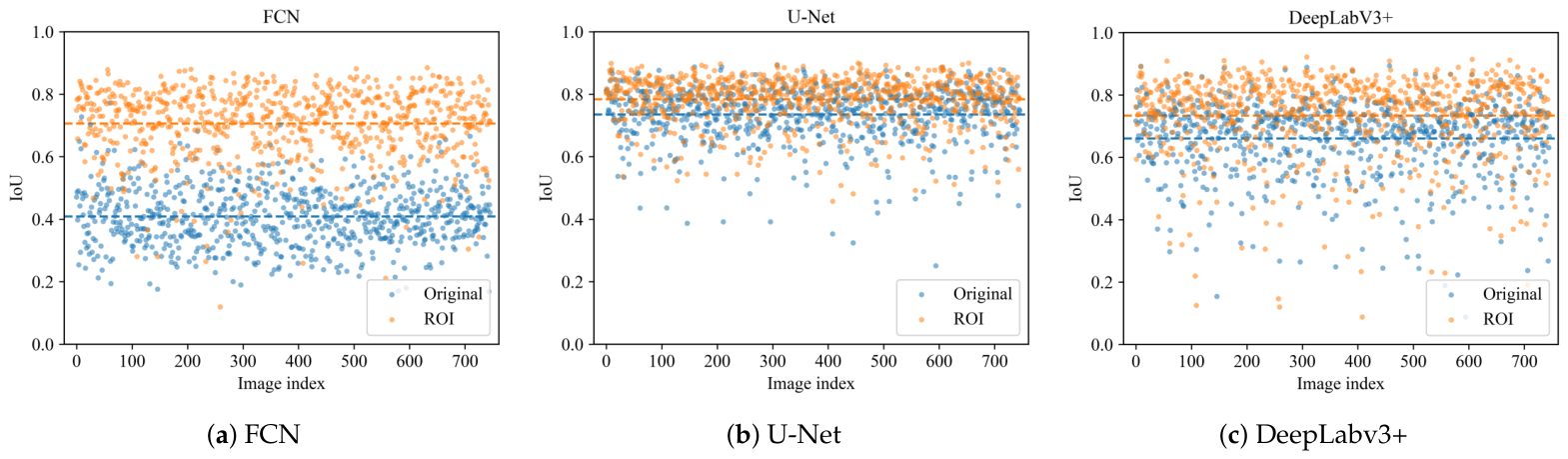
Comparison of IoU distributions between the original-image and ROI-based segmentation models.
Figure 10.
Comparison of IoU distributions between the original-image and ROI-based segmentation models.
Figure 11.
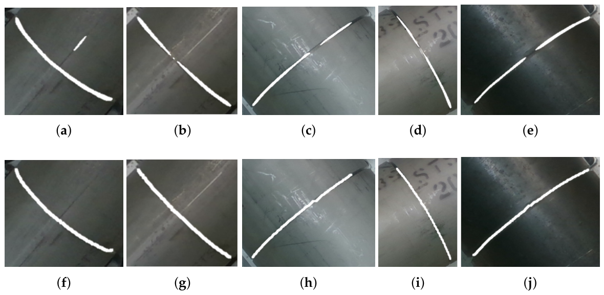
Comparison of weld seam segmentation results before and after image post-processing. (a–e) Raw segmentation outputs obtained from the detection module for five representative samples; (f–j) corresponding results after applying image post-processing.
Figure 11.
Comparison of weld seam segmentation results before and after image post-processing. (a–e) Raw segmentation outputs obtained from the detection module for five representative samples; (f–j) corresponding results after applying image post-processing.
Figure 12.
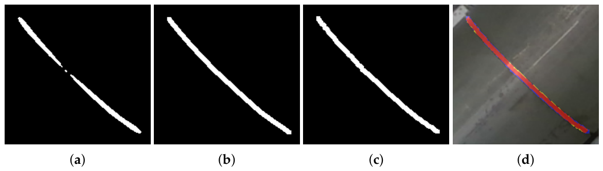
Comparison of post-processing results for weld seam mask images with and without consideration of discontinuous gaps. (a,e): Raw segmentation results predicted by the model; (b,f): post-processed results without considering the distance between broken weld segments; (c,g): post-processed results considering inter-segment distance by resizing and applying dilation; (d,h): final overlay images showing the corrected weld path on the original RGB image.
Figure 12.
Comparison of post-processing results for weld seam mask images with and without consideration of discontinuous gaps. (a,e): Raw segmentation results predicted by the model; (b,f): post-processed results without considering the distance between broken weld segments; (c,g): post-processed results considering inter-segment distance by resizing and applying dilation; (d,h): final overlay images showing the corrected weld path on the original RGB image.
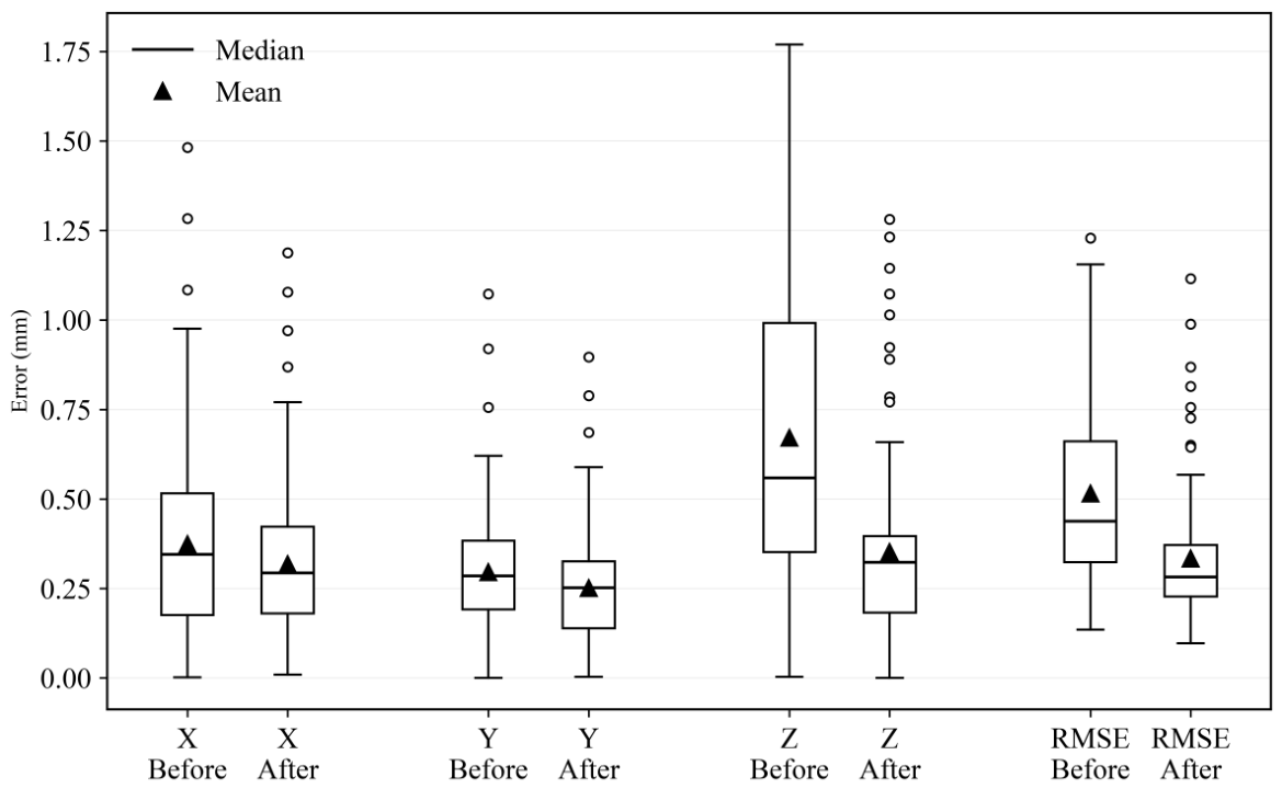
Figure 13.
Box plots of the X-, Y-, and Z-axes welding path errors and the overall RMSE before and after polynomial curve fitting, evaluated over all 88 corresponding weld seam points. The horizontal line and triangle represent the median and mean, respectively.
Figure 13.
Box plots of the X-, Y-, and Z-axes welding path errors and the overall RMSE before and after polynomial curve fitting, evaluated over all 88 corresponding weld seam points. The horizontal line and triangle represent the median and mean, respectively.
Figure 14.
Comparison of robotic welding results before and after polynomial fitting: (a) before polynomial fitting and (b) after polynomial fitting.
Figure 14.
Comparison of robotic welding results before and after polynomial fitting: (a) before polynomial fitting and (b) after polynomial fitting.
Table 1.
Average absolute coordinate error according to the number of depth frames used for averaging.
Table 1.
Average absolute coordinate error according to the number of depth frames used for averaging.
| Number of Frames | X Error (mm) | Y Error (mm) | Z Error (mm) |
|---|
| 1 | 10.745 | 6.982 | 6.558 |
| 10 | 7.373 | 4.348 | 7.472 |
| 25 | 5.830 | 2.298 | 5.620 |
| 50 | 0.023 | 0.176 | 4.631 |
| 100 | 0.012 | 0.031 | 3.938 |
Table 2.
Performance comparison of YOLOv8 model variants for weld seam ROI detection.
Table 2.
Performance comparison of YOLOv8 model variants for weld seam ROI detection.
| Model | Inference Time (ms/img) | Precision | Recall | | |
|---|
| YOLOv8-n | 8.7 | 0.996 | 1.000 | 0.995 | 0.731 |
| YOLOv8-s | 13.3 | 0.997 | 1.000 | 0.995 | 0.779 |
| YOLOv8-m | 19.7 | 0.998 | 1.000 | 0.995 | 0.750 |
| YOLOv8-l | 27.8 | 0.998 | 1.000 | 0.995 | 0.729 |
Table 3.
Repeatability evaluation of the manual RGB-to-depth registration parameters obtained by two operators over 15 repeated calibration trials.
Table 3.
Repeatability evaluation of the manual RGB-to-depth registration parameters obtained by two operators over 15 repeated calibration trials.
| Parameter | Operator 1 | Operator 2 |
|---|
| Scale ratio | | |
| X translation (pixel) | 19.53 ± 0.64 | 19.13 ± 0.35 |
| Y translation (pixel) | ± 0.26 | ± 0.92 |
| Rotation (°) | 0.109 ± 0.134 | 0.019 ± 0.078 |
Table 4.
Welding conditions used in the robotic welding experiments.
Table 4.
Welding conditions used in the robotic welding experiments.
| Parameter | Value |
|---|
| Welding process | Gas Metal Arc Welding (GMAW) |
| Welding power source | ABICOR BINZEL iROB Pulse 400 |
| Welding mode | Synergic mode |
| Base material | SS304, SS400 |
| Joint configuration | V-groove joint |
| Filler wire | KC-28 solid wire (EN ISO 14341-A G3Si1), (1.2 mm) |
| Shielding gas | 82% Ar + 18% |
| Welding current | 80 A |
| Arc voltage | 15.3–16.1 V (automatic in synergic mode) |
| Welding speed | 8 mm/s |
| Wire offset | 5 mm |
| Burn-back time | 0.25 s |
| Pipe configuration | Fixed pipe (non-rotary welding) |
| Robot | UR5e collaborative robot |
Table 5.
Composition of the pipe weld dataset, including SS304 and SS400 pipes of multiple diameters. A total of 1180 training images, 148 validation images, and 148 test images were used in this study.
Table 5.
Composition of the pipe weld dataset, including SS304 and SS400 pipes of multiple diameters. A total of 1180 training images, 148 validation images, and 148 test images were used in this study.
| Pipe Type | Outer Diameter | Train | Valid | Test |
|---|
| SS304 | 60.5 mm | 220 | 28 | 28 |
| 114.3 mm | 240 | 30 | 30 |
| 165.2 mm | 240 | 30 | 30 |
| SS400 | 114.3 mm | 240 | 30 | 30 |
| 165.2 mm | 240 | 30 | 30 |
| Total | | 1180 | 148 | 148 |
Table 6.
Performance comparison of segmentation models under different input conditions, including original images and ROI images.
Table 6.
Performance comparison of segmentation models under different input conditions, including original images and ROI images.
| Model | Input | IoU | Recall | 1-Precision |
|---|
| FCN | Original | | | |
| | ROI | | | |
| U-Net | Original | | | |
| | ROI | | | |
| DeepLabv3+ | Original | | | |
| | ROI | | | |
Table 7.
Comparison of segmentation performance after morphology-based post-processing over all test images. Values are reported as mean ± standard deviation.
Table 7.
Comparison of segmentation performance after morphology-based post-processing over all test images. Values are reported as mean ± standard deviation.
| Model | IoU | Recall | 1-Precision |
|---|
| FCN (ROI) | | | |
| FCN (ROI + Post) | | | |
| U-Net (ROI) | | | |
| U-Net (ROI + Post) | | | |
| DeepLabv3+ (ROI) | | | |
| DeepLabv3+ (ROI + Post) | | | |
Table 8.
Descriptive statistics of the welding path errors before and after polynomial curve fitting.
Table 8.
Descriptive statistics of the welding path errors before and after polynomial curve fitting.
| Metric | Stage | Mean ± SD (mm) | Min (mm) | Max (mm) |
|---|
| X | Before fitting | | 0.002 | 1.482 |
| X | After fitting | | 0.009 | 1.188 |
| Y | Before fitting | | 0.001 | 1.072 |
| Y | After fitting | | 0.003 | 0.896 |
| Z | Before fitting | | 0.003 | 1.769 |
| Z | After fitting | | 0.000 | 1.281 |
| RMSE | Before fitting | | 0.135 | 1.229 |
| RMSE | After fitting | | 0.097 | 1.115 |