Figure 1.
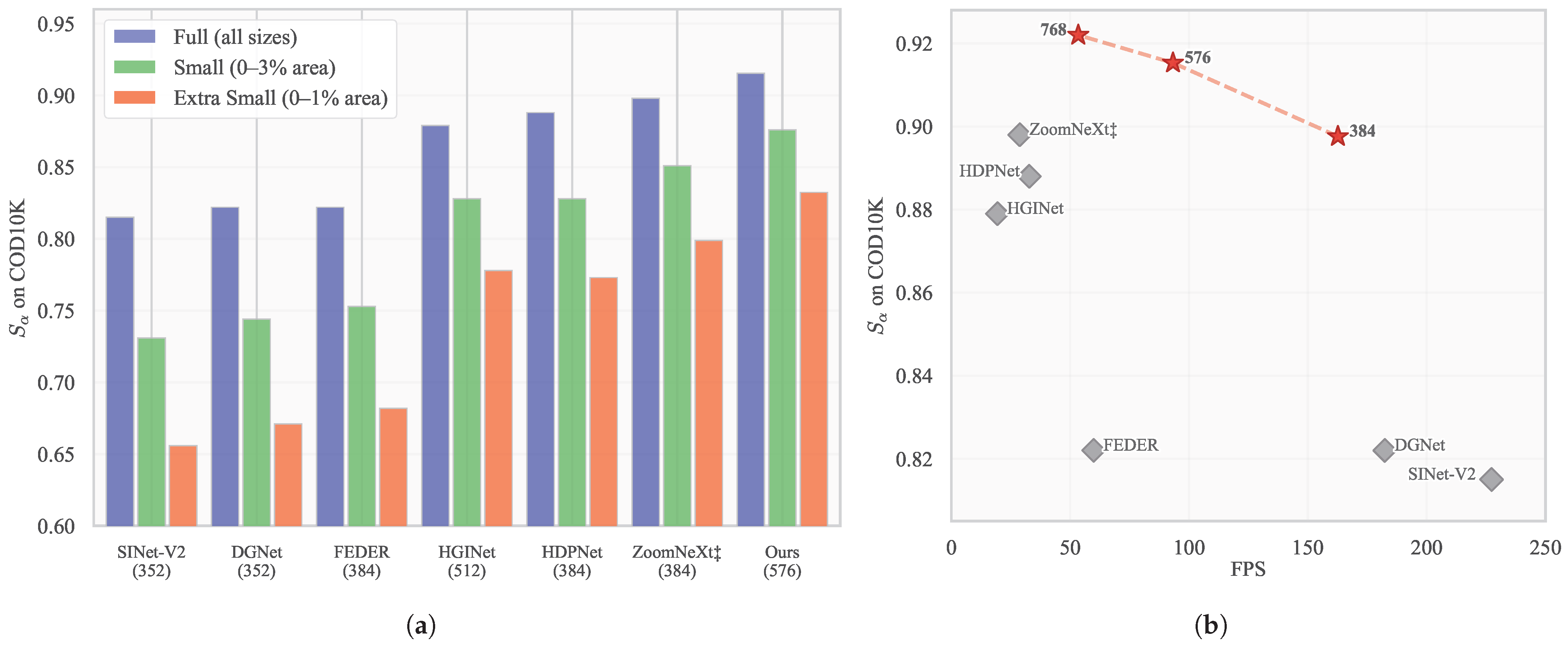
Performance comparison of LeanCOD with existing COD methods on COD10K. (a) Performance across small-object regimes. Small and extra-small objects exhibit larger degradation than the full test set, while LeanCOD reduces this degradation. Parenthesized numbers denote input resolutions. (b) Performance–FPS comparison on an RTX 4090. Gray points denote existing methods, and red stars denote LeanCOD at 384, 576, and 768 input resolutions. LeanCOD improves accuracy with increasing resolution while maintaining competitive throughput, showing the trade-off between accuracy and throughput. ‡ Tri-scale inference.
Figure 1.
Performance comparison of LeanCOD with existing COD methods on COD10K. (a) Performance across small-object regimes. Small and extra-small objects exhibit larger degradation than the full test set, while LeanCOD reduces this degradation. Parenthesized numbers denote input resolutions. (b) Performance–FPS comparison on an RTX 4090. Gray points denote existing methods, and red stars denote LeanCOD at 384, 576, and 768 input resolutions. LeanCOD improves accuracy with increasing resolution while maintaining competitive throughput, showing the trade-off between accuracy and throughput. ‡ Tri-scale inference.
Figure 2.
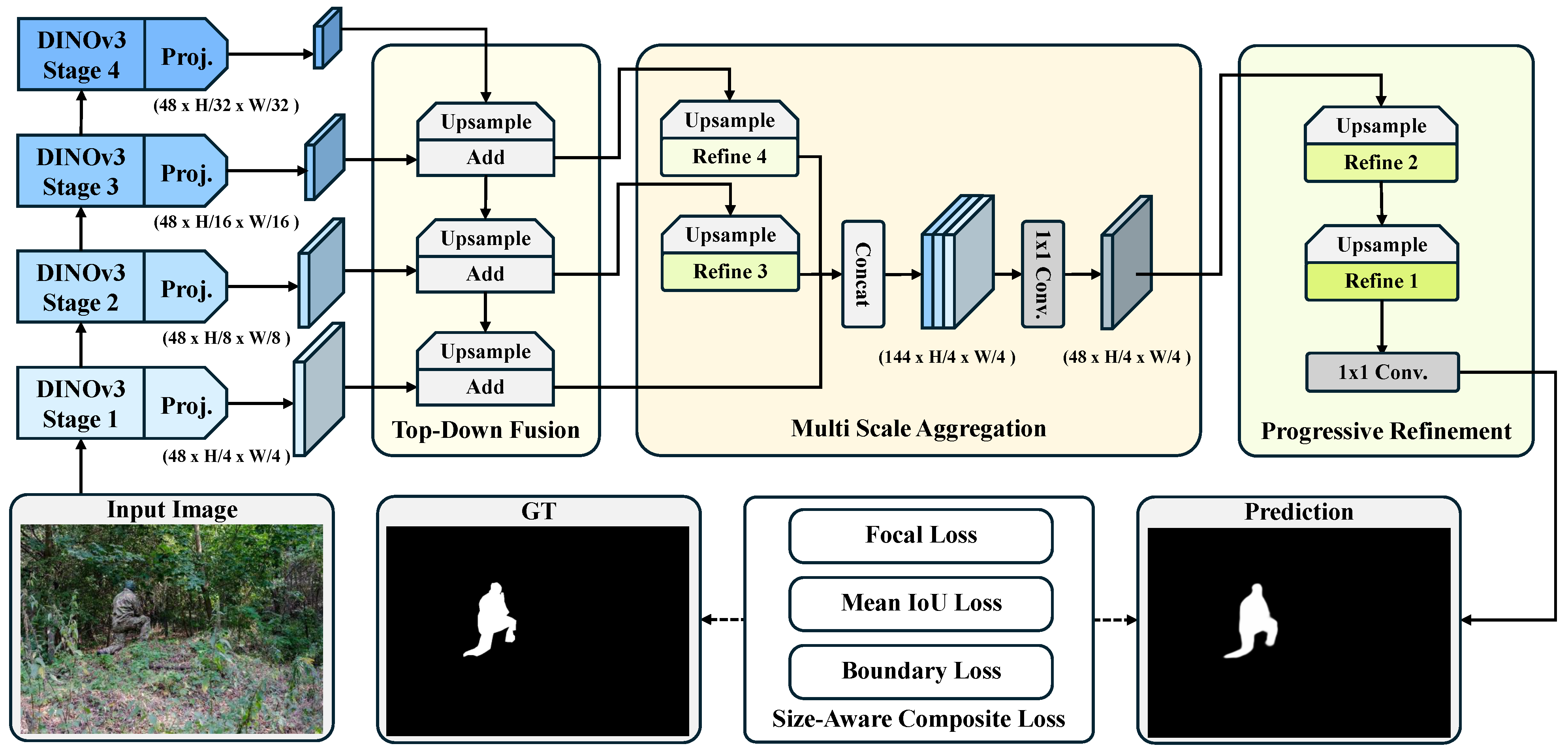
Overall framework of LeanCOD. The DINOv3-ConvNeXt encoder (left) extracts four feature maps with resolutions ranging from to . These features are projected to a 48-channel dimension. The top-down fusion module integrates semantic context from deep to shallow scales using bilinear upsampling and element-wise addition. The three fused maps are concatenated at the resolution and compressed by a 1 × 1 convolution in the aggregation block. Finally, the refinement stage progressively restores the spatial resolution to H × W to generate the prediction map, supervised by the size-aware composite loss. Solid arrows denote the forward data flow, and dashed arrows indicate supervision signals from the loss function. Color gradients illustrate the progressive processing within each stage.
Figure 2.
Overall framework of LeanCOD. The DINOv3-ConvNeXt encoder (left) extracts four feature maps with resolutions ranging from to . These features are projected to a 48-channel dimension. The top-down fusion module integrates semantic context from deep to shallow scales using bilinear upsampling and element-wise addition. The three fused maps are concatenated at the resolution and compressed by a 1 × 1 convolution in the aggregation block. Finally, the refinement stage progressively restores the spatial resolution to H × W to generate the prediction map, supervised by the size-aware composite loss. Solid arrows denote the forward data flow, and dashed arrows indicate supervision signals from the loss function. Color gradients illustrate the progressive processing within each stage.
Figure 3.
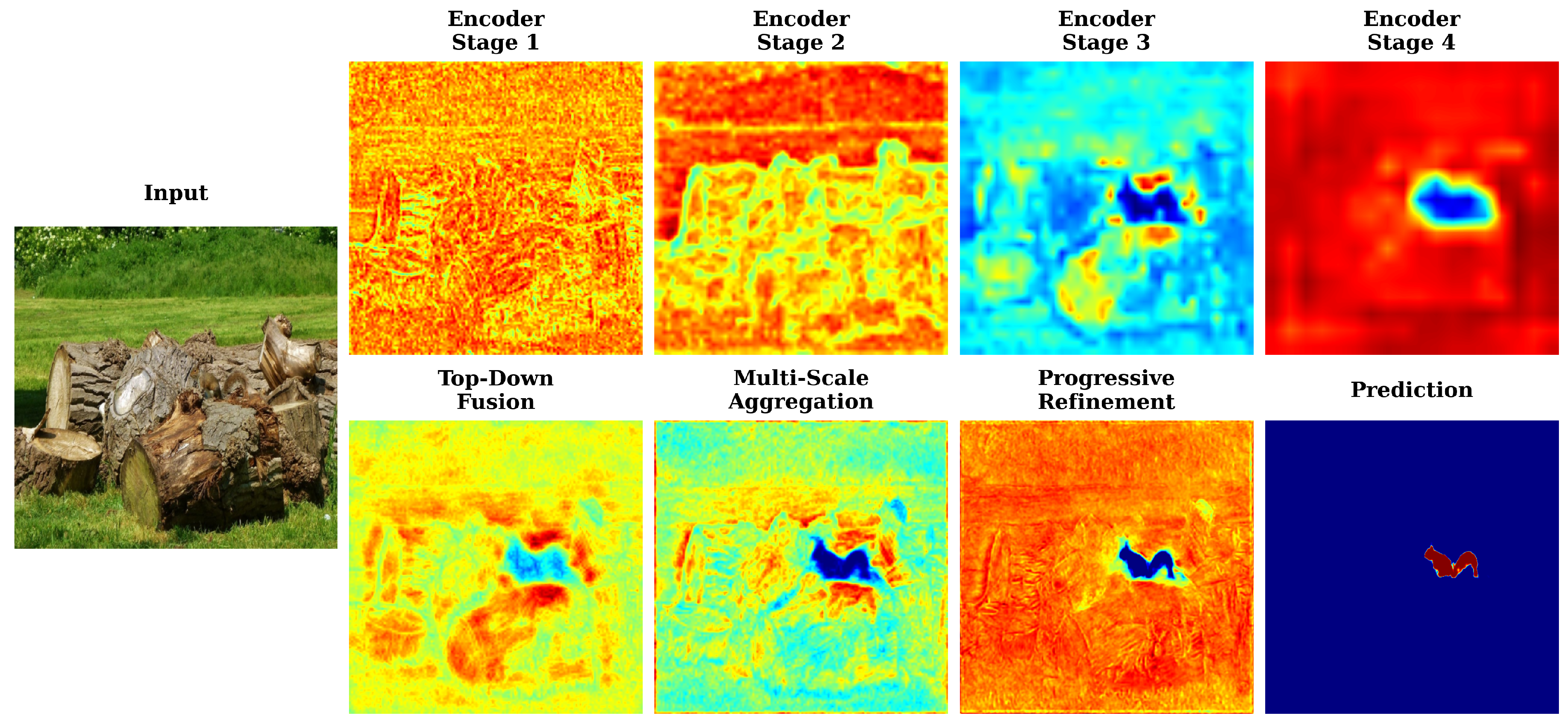
Feature flow visualization of LeanCOD. Early encoder stages capture fine spatial textures, while deeper stages yield robust semantic representations of camouflaged targets. Through top-down fusion, aggregation, and progressive refinement, the decoder propagates the localized target response back to higher spatial resolutions and produces a compact final prediction. Each panel shows the first principal component of feature activations computed by Eigen-CAM, ranging from blue for low values to red for high values.
Figure 3.
Feature flow visualization of LeanCOD. Early encoder stages capture fine spatial textures, while deeper stages yield robust semantic representations of camouflaged targets. Through top-down fusion, aggregation, and progressive refinement, the decoder propagates the localized target response back to higher spatial resolutions and produces a compact final prediction. Each panel shows the first principal component of feature activations computed by Eigen-CAM, ranging from blue for low values to red for high values.
Figure 4.
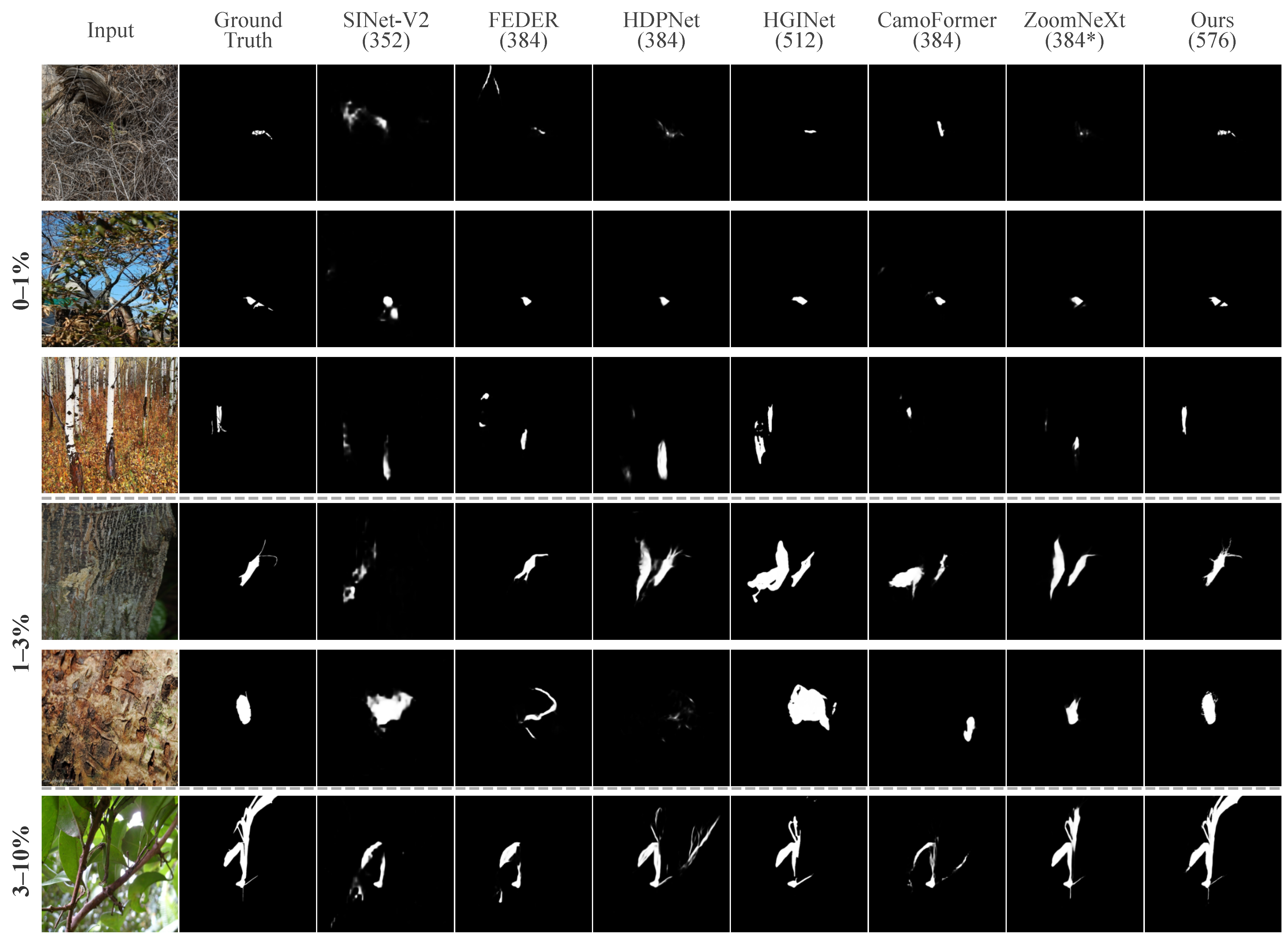
Qualitative comparison on COD10K samples grouped by object area ratio. Rows are organized into three size groups (0–1%, 1–3%, and 3–10%), separated by dashed lines. Columns: input, ground truth, and predictions from six methods. Parenthesized numbers denote input resolution. * denotes tri-scale inference.
Figure 4.
Qualitative comparison on COD10K samples grouped by object area ratio. Rows are organized into three size groups (0–1%, 1–3%, and 3–10%), separated by dashed lines. Columns: input, ground truth, and predictions from six methods. Parenthesized numbers denote input resolution. * denotes tri-scale inference.
Figure 5.
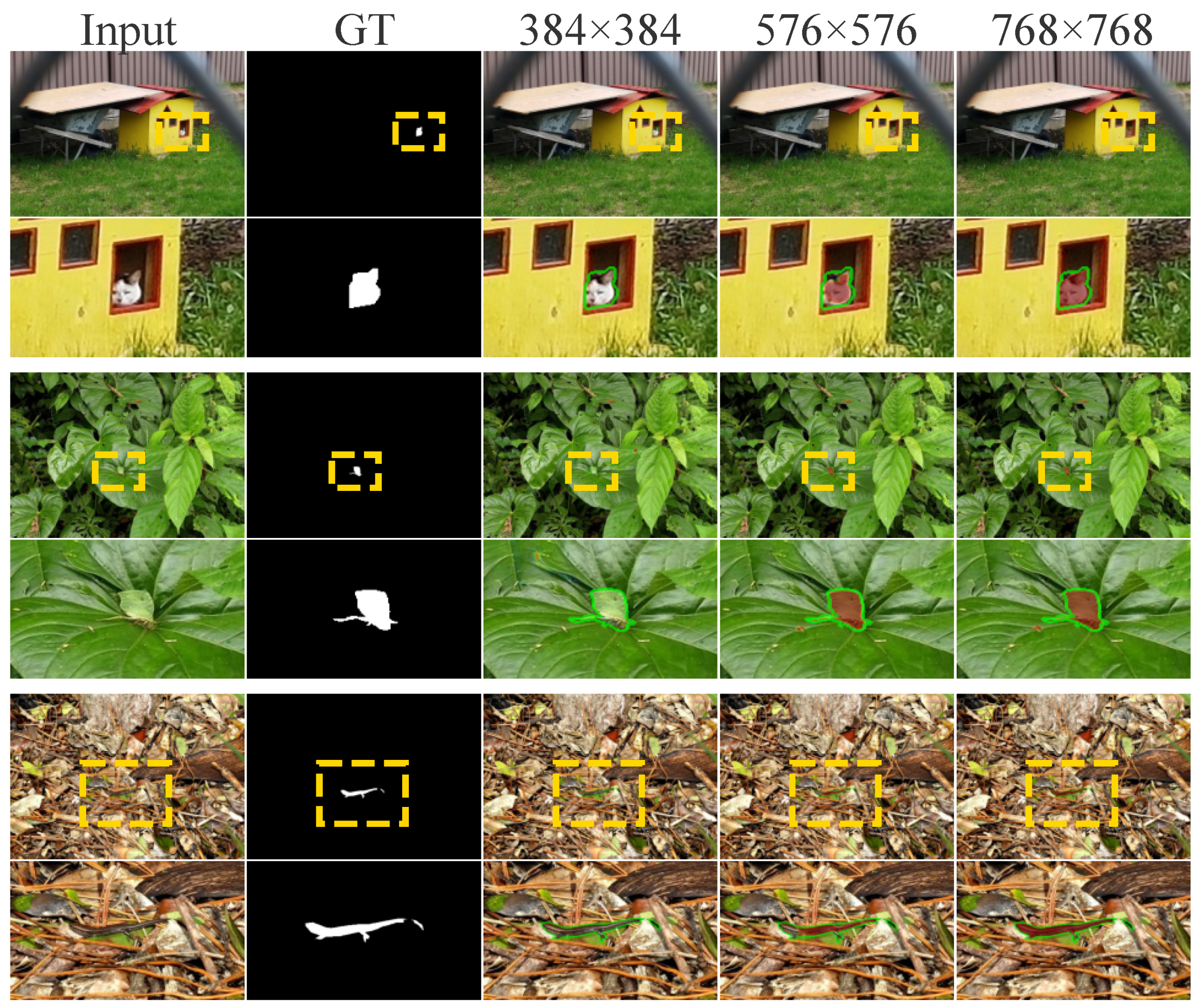
Resolution scaling on three extra-small-object samples (0–1% area) from COD10K. Each example presents the full image, zoomed crop, prediction overlay, and ground-truth boundary in green. Segmentation quality improves progressively as the input resolution increases from 384 to 768. Yellow dashed boxes indicate the zoomed region of interest, and green contours denote the ground-truth boundary.
Figure 5.
Resolution scaling on three extra-small-object samples (0–1% area) from COD10K. Each example presents the full image, zoomed crop, prediction overlay, and ground-truth boundary in green. Segmentation quality improves progressively as the input resolution increases from 384 to 768. Yellow dashed boxes indicate the zoomed region of interest, and green contours denote the ground-truth boundary.
Figure 6.
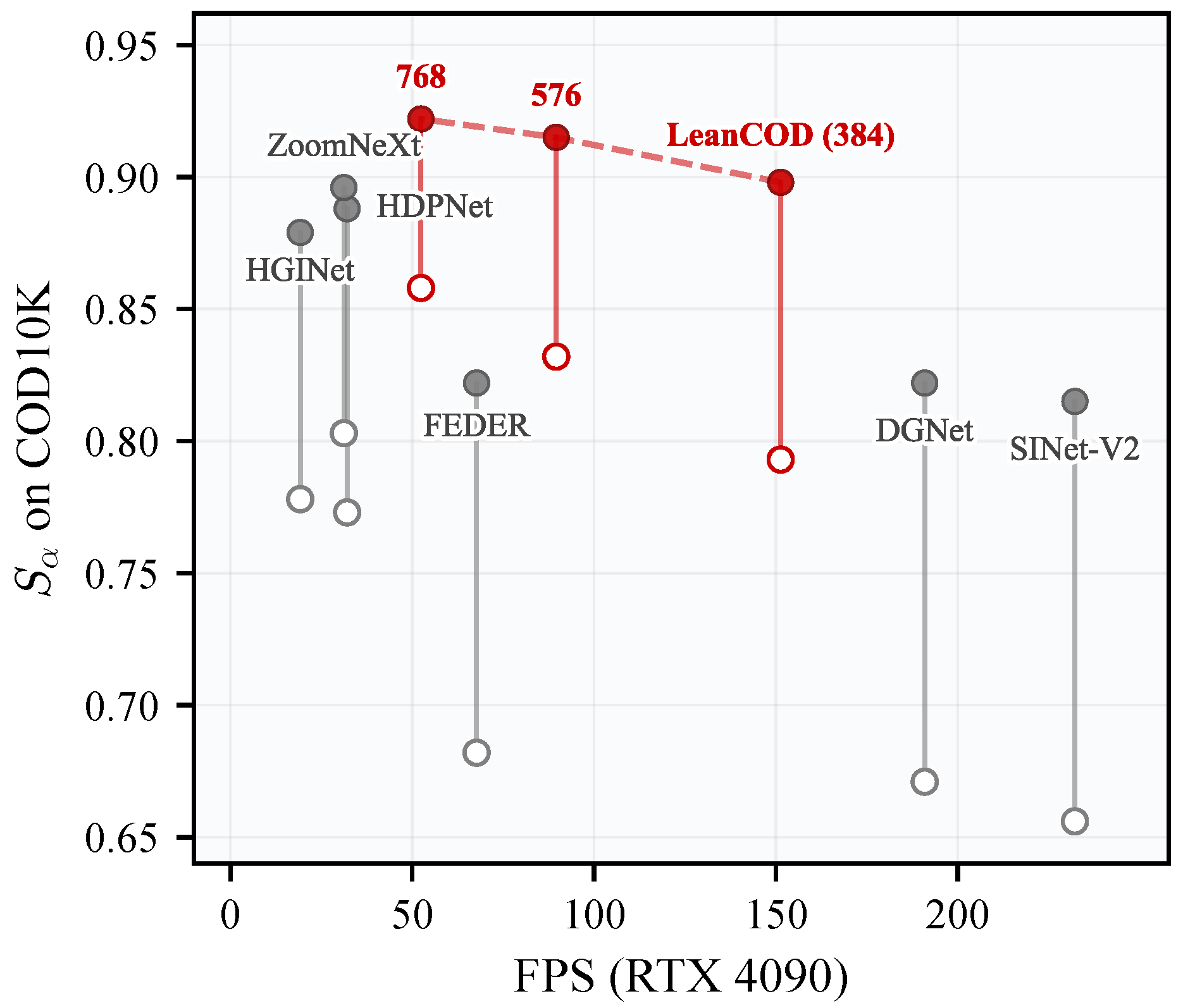
Speed vs. overall and extra-small on RTX 4090 (COD10K). Filled: overall ; hollow: extra-small (0–1%) ; vertical lines: degradation gap. Red points denote LeanCOD at 384, 576, and 768 input resolutions.
Figure 6.
Speed vs. overall and extra-small on RTX 4090 (COD10K). Filled: overall ; hollow: extra-small (0–1%) ; vertical lines: degradation gap. Red points denote LeanCOD at 384, 576, and 768 input resolutions.
Figure 7.
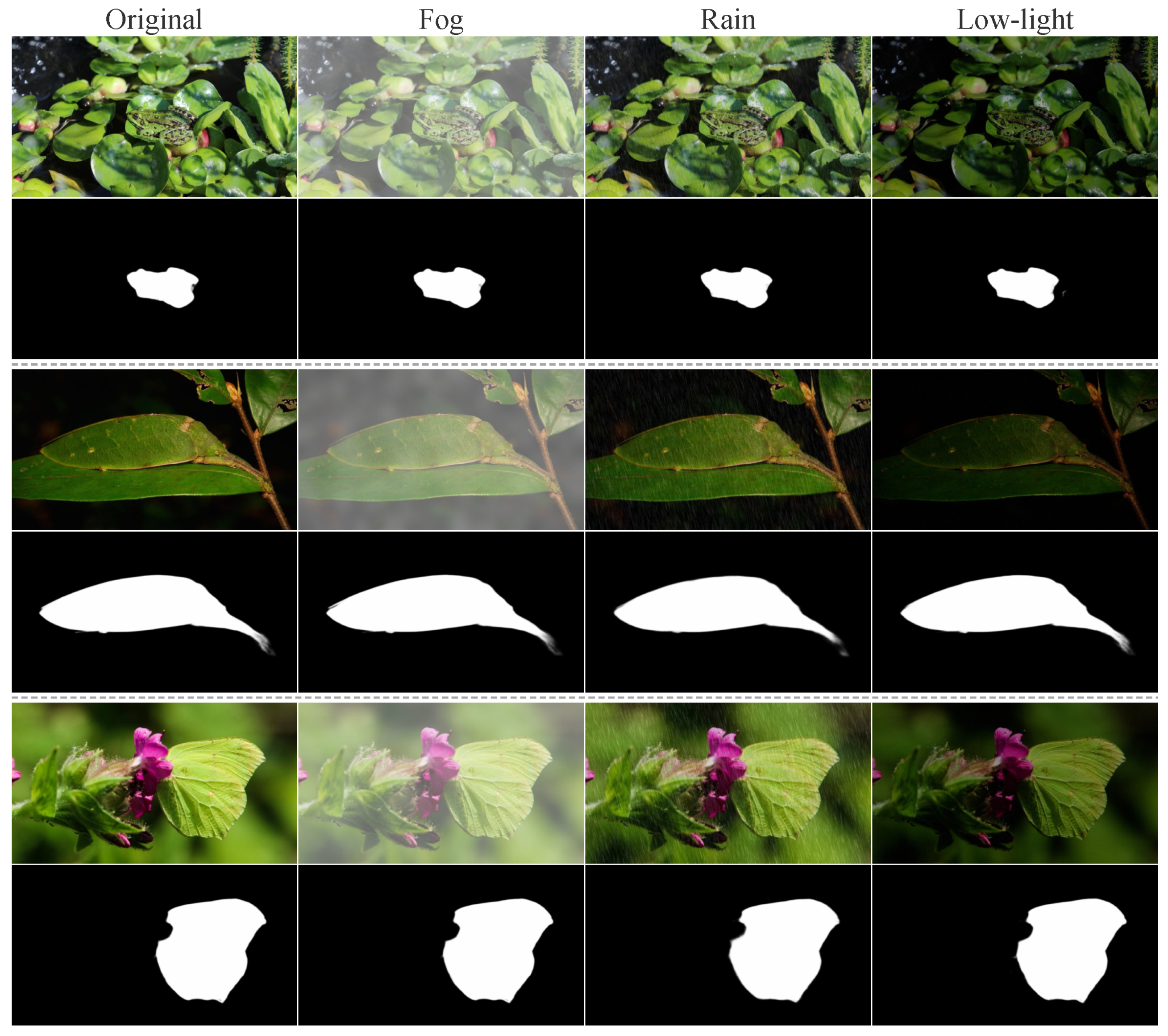
Qualitative results under synthetic adverse conditions on COD10K. Each row pair shows the input image and the predicted mask from LeanCOD. Columns denote original, fog, rain, and low-light conditions. Object location and overall shape are preserved across conditions, although some rain and low-light inputs show weaker interior responses.
Figure 7.
Qualitative results under synthetic adverse conditions on COD10K. Each row pair shows the input image and the predicted mask from LeanCOD. Columns denote original, fog, rain, and low-light conditions. Object location and overall shape are preserved across conditions, although some rain and low-light inputs show weaker interior responses.
Table 1.
Comparison with state-of-the-art methods on four COD benchmarks. † Results are reported by the original papers. § Results are evaluated from official weights using our evaluation code. †§ Results are paper-reported for CAMO/COD10K/NC4K and evaluated by us for CHAMELEON. ‡ Tri-scale inference. †‡ Results are reported by the original paper using tri-scale inference. The first three methods are lightweight baselines listed as an efficiency-oriented reference. The LeanCOD rows at 576 and 768 are listed as a resolution-scaling extension and are not used for rank marking. The arrows indicate whether higher (↑) or lower (↓) values are better. – indicates that the result is not reported in the original paper. Bold and underlined values indicate the best and second-best results, respectively.
Table 1.
Comparison with state-of-the-art methods on four COD benchmarks. † Results are reported by the original papers. § Results are evaluated from official weights using our evaluation code. †§ Results are paper-reported for CAMO/COD10K/NC4K and evaluated by us for CHAMELEON. ‡ Tri-scale inference. †‡ Results are reported by the original paper using tri-scale inference. The first three methods are lightweight baselines listed as an efficiency-oriented reference. The LeanCOD rows at 576 and 768 are listed as a resolution-scaling extension and are not used for rank marking. The arrows indicate whether higher (↑) or lower (↓) values are better. – indicates that the result is not reported in the original paper. Bold and underlined values indicate the best and second-best results, respectively.
| Method | Venue | Res. | CHAMELEON (76) | CAMO (250) | COD10K (2026) | NC4K (4121) |
|---|
| | | MAE ↓ | | | | MAE ↓ | | | | MAE ↓ | | | | MAE ↓ |
|---|
| TinyCOD † [19] | ICASSP’23 | 384 | 0.887 | 0.931 | 0.814 | 0.030 | 0.822 | 0.890 | 0.752 | 0.066 | 0.811 | 0.877 | 0.678 | 0.036 | 0.843 | 0.903 | 0.766 | 0.047 |
| DGNet-S † [12] | MIR’22 | 352 | – | – | – | – | 0.826 | 0.896 | 0.754 | 0.063 | 0.810 | 0.869 | 0.672 | 0.036 | 0.845 | 0.902 | 0.764 | 0.047 |
| LiteCOD † [8] | AI’25 | 512 | – | – | – | – | 0.841 | 0.907 | 0.796 | 0.056 | 0.852 | 0.920 | 0.765 | 0.026 | 0.870 | 0.926 | 0.822 | 0.036 |
| SINet-v2 † [5] | TPAMI’22 | 352 | 0.888 | 0.942 | 0.882 | 0.030 | 0.820 | 0.882 | 0.743 | 0.070 | 0.815 | 0.887 | 0.680 | 0.037 | 0.847 | 0.903 | 0.770 | 0.048 |
| DGNet † [12] | MIR’22 | 352 | 0.891 | 0.952 | 0.838 | 0.024 | 0.839 | 0.901 | 0.769 | 0.057 | 0.822 | 0.903 | 0.693 | 0.033 | 0.857 | 0.907 | 0.784 | 0.042 |
| FEDER † [3] | CVPR’23 | 384 | 0.894 | 0.947 | 0.855 | 0.028 | 0.807 | 0.873 | 0.785 | 0.069 | 0.823 | 0.900 | 0.740 | 0.032 | 0.846 | 0.905 | 0.789 | 0.045 |
| FSPNet † [10] | CVPR’23 | 384 | 0.908 | 0.965 | 0.851 | 0.023 | 0.856 | 0.899 | 0.799 | 0.050 | 0.851 | 0.895 | 0.735 | 0.026 | 0.879 | 0.915 | 0.816 | 0.035 |
| CamoFormer § [2] | TPAMI’24 | 384 | 0.910 | 0.970 | 0.866 | 0.022 | 0.872 | 0.931 | 0.831 | 0.046 | 0.869 | 0.931 | 0.786 | 0.023 | 0.892 | 0.941 | 0.847 | 0.030 |
| ZoomNeXt †‡ [6] | TPAMI’24 | 384 ‡ | 0.924 | 0.975 | 0.896 | 0.018 | 0.889 | 0.945 | 0.875 | 0.041 | 0.898 | 0.956 | 0.848 | 0.018 | 0.903 | 0.951 | 0.863 | 0.028 |
| HGINet † [4] | TIP’24 | 512 | 0.915 | 0.970 | 0.889 | 0.018 | 0.874 | 0.937 | 0.848 | 0.041 | 0.882 | 0.949 | 0.821 | 0.019 | 0.894 | 0.947 | 0.865 | 0.027 |
| FGSA-Net † [32] | TMM’25 | 512 | 0.916 | 0.975 | 0.903 | 0.016 | 0.889 | 0.944 | 0.870 | 0.036 | 0.893 | 0.953 | 0.849 | 0.015 | 0.903 | 0.951 | 0.883 | 0.023 |
| HDPNet †§ [11] | WACV’25 | 384 | 0.922 | 0.943 | 0.861 | 0.021 | 0.893 | 0.934 | 0.851 | 0.040 | 0.888 | 0.925 | 0.794 | 0.020 | 0.902 | 0.950 | 0.850 | 0.029 |
| ESCNet † [33] | ICCV’25 | 416 | – | – | – | – | 0.871 | 0.934 | 0.843 | 0.044 | 0.873 | 0.939 | 0.804 | 0.021 | 0.892 | 0.941 | 0.859 | 0.028 |
| Ours | – | 384 | 0.925 | 0.969 | 0.871 | 0.020 | 0.904 | 0.949 | 0.870 | 0.035 | 0.898 | 0.944 | 0.824 | 0.018 | 0.910 | 0.958 | 0.870 | 0.026 |
| Ours (high-res) | – | 576 | 0.935 | 0.974 | 0.895 | 0.018 | 0.911 | 0.953 | 0.881 | 0.033 | 0.915 | 0.956 | 0.859 | 0.016 | 0.915 | 0.959 | 0.881 | 0.026 |
| Ours (high-res) | – | 768 | 0.937 | 0.971 | 0.901 | 0.017 | 0.913 | 0.952 | 0.885 | 0.033 | 0.922 | 0.961 | 0.874 | 0.015 | 0.916 | 0.959 | 0.884 | 0.025 |
Table 2.
Size-wise performance on the COD10K test set. All external methods use official pretrained weights under identical evaluation. ; smaller indicates better robustness to small objects. ‡ Tri-scale inference (0.5× + 1× + 1.5× of nominal resolution, e.g., 192 + 384 + 576 for 384). The LeanCOD rows at 576 and 768 are used as a resolution-scaling extension. The arrows indicate whether higher (↑) values are better.
Table 2.
Size-wise performance on the COD10K test set. All external methods use official pretrained weights under identical evaluation. ; smaller indicates better robustness to small objects. ‡ Tri-scale inference (0.5× + 1× + 1.5× of nominal resolution, e.g., 192 + 384 + 576 for 384). The LeanCOD rows at 576 and 768 are used as a resolution-scaling extension. The arrows indicate whether higher (↑) values are better.
| Method | Venue | Res. | | by Object Area Ratio (%) | |
|---|
| Full | >25 | 10–25 | 5–10 | 3–5 | 1–3 | 0–1 | |
|---|
| SINet-v2 [5] | TPAMI’22 | 352 | 0.815 | 0.845 | 0.873 | 0.841 | 0.825 | 0.767 | 0.656 | −0.159 |
| DGNet [12] | MIR’22 | 352 | 0.822 | 0.855 | 0.875 | 0.850 | 0.823 | 0.779 | 0.671 | −0.151 |
| FEDER [3] | CVPR’23 | 384 | 0.822 | 0.825 | 0.866 | 0.849 | 0.835 | 0.786 | 0.682 | −0.140 |
| CamoFormer [2] | TPAMI’24 | 384 | 0.869 | 0.892 | 0.912 | 0.894 | 0.869 | 0.833 | 0.748 | −0.121 |
| HGINet [4] | TIP’24 | 512 | 0.879 | 0.891 | 0.912 | 0.901 | 0.879 | 0.851 | 0.778 | −0.101 |
| HDPNet [11] | WACV’25 | 384 | 0.888 | 0.905 | 0.925 | 0.911 | 0.894 | 0.854 | 0.773 | −0.115 |
| ESCNet [33] | ICCV’25 | 416 | 0.874 | 0.891 | 0.910 | 0.897 | 0.882 | 0.843 | 0.753 | −0.121 |
| ZoomNeXt ‡ [6] | TPAMI’24 | 384 ‡ | 0.898 | 0.901 | 0.927 | 0.920 | 0.901 | 0.875 | 0.799 | −0.099 |
| Ours | – | 384 | 0.898 | 0.910 | 0.929 | 0.919 | 0.905 | 0.871 | 0.793 | −0.105 |
| Ours (high-res) | – | 576 | 0.915 | 0.914 | 0.937 | 0.934 | 0.922 | 0.897 | 0.832 | −0.083 |
| Ours (high-res) | – | 768 | 0.922 | 0.917 | 0.940 | 0.937 | 0.928 | 0.908 | 0.858 | −0.064 |
Table 3.
Size-wise performance on the COD10K test set. is reported alongside as it is particularly sensitive to small-object boundary quality. ; smaller indicates better robustness to scale variation. ‡ Tri-scale inference. The LeanCOD rows at 576 and 768 are used as a resolution-scaling extension. The arrows indicate whether higher (↑) values are better.
Table 3.
Size-wise performance on the COD10K test set. is reported alongside as it is particularly sensitive to small-object boundary quality. ; smaller indicates better robustness to scale variation. ‡ Tri-scale inference. The LeanCOD rows at 576 and 768 are used as a resolution-scaling extension. The arrows indicate whether higher (↑) values are better.
| Method | Venue | Res. | | by Object Area Ratio (%) | |
|---|
| Full | >25 | 10–25 | 5–10 | 3–5 | 1–3 | 0–1 | |
|---|
| SINet-v2 [5] | TPAMI’22 | 352 | 0.680 | 0.843 | 0.815 | 0.728 | 0.682 | 0.556 | 0.326 | −0.354 |
| DGNet [12] | MIR’22 | 352 | 0.692 | 0.852 | 0.821 | 0.746 | 0.680 | 0.573 | 0.349 | −0.343 |
| FEDER [3] | CVPR’23 | 384 | 0.715 | 0.832 | 0.824 | 0.768 | 0.729 | 0.614 | 0.384 | −0.331 |
| CamoFormer [2] | TPAMI’24 | 384 | 0.786 | 0.896 | 0.884 | 0.832 | 0.781 | 0.698 | 0.516 | −0.270 |
| HGINet [4] | TIP’24 | 512 | 0.815 | 0.913 | 0.897 | 0.854 | 0.812 | 0.740 | 0.579 | −0.236 |
| HDPNet [11] | WACV’25 | 384 | 0.794 | 0.909 | 0.892 | 0.842 | 0.798 | 0.701 | 0.503 | −0.291 |
| ESCNet [33] | ICCV’25 | 416 | 0.808 | 0.913 | 0.894 | 0.853 | 0.818 | 0.729 | 0.533 | −0.275 |
| ZoomNeXt ‡ [6] | TPAMI’24 | 384 ‡ | 0.827 | 0.912 | 0.904 | 0.868 | 0.825 | 0.762 | 0.585 | −0.242 |
| Ours | – | 384 | 0.824 | 0.915 | 0.899 | 0.864 | 0.831 | 0.752 | 0.593 | −0.231 |
| Ours (high-res) | – | 576 | 0.859 | 0.919 | 0.916 | 0.892 | 0.863 | 0.809 | 0.675 | −0.184 |
| Ours (high-res) | – | 768 | 0.874 | 0.924 | 0.921 | 0.898 | 0.878 | 0.834 | 0.724 | −0.150 |
Table 4.
Resolution-ordered efficiency and COD10K accuracy comparison on an RTX 4090. We select SINet-V2 and DGNet as high-throughput representatives and ZoomNeXt as a high-accuracy representative for cross-resolution comparison. All measurements use identical settings: batch size 1, 50 warm-up iterations, and 200 timed runs. Peak memory denotes the maximum CUDA memory allocated during inference. ‡ indicates tri-scale inference (0.5× + 1.0× + 1.5× of nominal resolution). ★ indicates models retrained by us at the listed resolution using the same optimizer, loss, and augmentation as the original papers; these are not the published models and serve as diagnostic baselines. Extra-small denotes the 0–1% object-area-ratio bin of COD10K. The arrows indicate whether higher (↑) or lower (↓) values are better.
Table 4.
Resolution-ordered efficiency and COD10K accuracy comparison on an RTX 4090. We select SINet-V2 and DGNet as high-throughput representatives and ZoomNeXt as a high-accuracy representative for cross-resolution comparison. All measurements use identical settings: batch size 1, 50 warm-up iterations, and 200 timed runs. Peak memory denotes the maximum CUDA memory allocated during inference. ‡ indicates tri-scale inference (0.5× + 1.0× + 1.5× of nominal resolution). ★ indicates models retrained by us at the listed resolution using the same optimizer, loss, and augmentation as the original papers; these are not the published models and serve as diagnostic baselines. Extra-small denotes the 0–1% object-area-ratio bin of COD10K. The arrows indicate whether higher (↑) or lower (↓) values are better.
| | | Complexity | RTX 4090 | COD10K |
|---|
| Method | Res. | Params ↓ | GFLOPs ↓ | FPS ↑ | Peak Mem. (MB) ↓ | Full ↑ | Extra-Small ↑ |
|---|
| SINet-v2 [5] | 352 | 26.98 M | 24.3 | 232.2 | 136.1 | 0.815 | 0.656 |
| DGNet [12] | 352 | 19.22 M | 12.8 | 190.9 | 132.6 | 0.822 | 0.671 |
| ZoomNeXt ‡ [6] | 384 ‡ | 65.37 M | 264.1 | 31.2 | 404.9 | 0.896 | 0.803 |
| Ours | 384 | 88.43 M | 96.5 | 151.3 | 420.8 | 0.898 | 0.793 |
| SINet-v2 ★ [5] | 576 | 26.98 M | 65.2 | 213.9 | 192.8 | 0.840 | 0.701 |
| DGNet ★ [12] | 576 | 19.22 M | 34.1 | 178.0 | 234.6 | 0.862 | 0.742 |
| ZoomNeXt ‡ [6] | 576 ‡ | 65.37 M | 686.7 | 16.1 | 591.2 | 0.900 | 0.831 |
| Ours | 576 | 88.43 M | 217.1 | 89.6 | 511.2 | 0.915 | 0.832 |
| SINet-v2 ★ [5] | 768 | 26.98 M | 115.9 | 152.2 | 258.0 | 0.843 | 0.716 |
| DGNet ★ [12] | 768 | 19.22 M | 60.7 | 113.9 | 357.1 | 0.869 | 0.750 |
| ZoomNeXt ‡ [6] | 768 ‡ | 65.37 M | 1451.1 | 8.5 | 845.8 | 0.889 | 0.825 |
| Ours | 768 | 88.43 M | 385.9 | 52.4 | 640.4 | 0.922 | 0.858 |
Table 5.
Robustness evaluation under synthetic COD10K corruptions using LeanCOD at a input resolution. The fog, rain, and low-light conditions are evaluation-only input variants that reuse the original COD10K ground-truth masks; no adverse-condition images are used for training, fine-tuning, or inference-time adaptation. denotes the change from the original condition; smaller indicates better stability under the corruption. Rain produces the largest drop ( on full COD10K), while fog and low light yield smaller changes. The arrows indicate whether higher (↑) or lower (↓) values are better. – in the column indicates the reference condition.
Table 5.
Robustness evaluation under synthetic COD10K corruptions using LeanCOD at a input resolution. The fog, rain, and low-light conditions are evaluation-only input variants that reuse the original COD10K ground-truth masks; no adverse-condition images are used for training, fine-tuning, or inference-time adaptation. denotes the change from the original condition; smaller indicates better stability under the corruption. Rain produces the largest drop ( on full COD10K), while fog and low light yield smaller changes. The arrows indicate whether higher (↑) or lower (↓) values are better. – in the column indicates the reference condition.
| Condition | COD10K Full | Extra-Small (0–1%) |
|---|
| | MAE ↓ | | | | MAE ↓ | |
|---|
| Original | 0.9153 | 0.8590 | 0.0158 | – | 0.8324 | 0.6746 | 0.0043 | – |
| Fog | 0.9101 | 0.8519 | 0.0165 | | 0.8259 | 0.6605 | 0.0040 | |
| Rain | 0.8908 | 0.8194 | 0.0207 | | 0.8074 | 0.6306 | 0.0058 | |
| Low Light | 0.9028 | 0.8403 | 0.0176 | | 0.8135 | 0.6430 | 0.0051 | |
Table 6.
Backbone comparison on COD10K with the LeanCOD decoder fixed. All models are trained for 100 epochs at input resolution. Backbones are grouped by architecture family. Extra-small denotes the 0–1% object-area-ratio subset of COD10K (188 images). CN denotes ConvNeXt. The arrows indicate whether higher (↑) or lower (↓) values are better. Best results are shown in bold, and second-best results are underlined.
Table 6.
Backbone comparison on COD10K with the LeanCOD decoder fixed. All models are trained for 100 epochs at input resolution. Backbones are grouped by architecture family. Extra-small denotes the 0–1% object-area-ratio subset of COD10K (188 images). CN denotes ConvNeXt. The arrows indicate whether higher (↑) or lower (↓) values are better. Best results are shown in bold, and second-best results are underlined.
| | | | | COD10K Full | Extra-Small (0–1%) |
|---|
| Backbone | Params ↓ | GFLOPs ↓ | FPS ↑ | | | | |
|---|
| EfficientNet-B1 | 6.62 M | 8.74 | 236.7 | 0.819 | 0.640 | 0.686 | 0.335 |
| EfficientNet-B4 | 17.66 M | 14.13 | 184.2 | 0.838 | 0.684 | 0.708 | 0.400 |
| ResNet-50 | 23.77 M | 29.93 | 458.4 | 0.820 | 0.668 | 0.690 | 0.368 |
| ResNet-101 | 42.76 M | 51.75 | 299.8 | 0.837 | 0.685 | 0.707 | 0.397 |
| PVTv2-B2 | 24.98 M | 30.88 | 223.2 | 0.863 | 0.748 | 0.735 | 0.463 |
| PVTv2-B3 | 44.86 M | 48.60 | 153.2 | 0.876 | 0.769 | 0.746 | 0.486 |
| PVTv2-B4 | 62.17 M | 68.51 | 112.1 | 0.879 | 0.776 | 0.760 | 0.514 |
| PVTv2-B5 | 81.57 M | 78.69 | 89.2 | 0.877 | 0.775 | 0.759 | 0.510 |
| DINOv3-ViT-S | 22.12 M | 37.71 | 232.2 | 0.869 | 0.741 | 0.741 | 0.471 |
| DINOv3-CN-Tiny | 28.50 M | 32.26 | 350.5 | 0.871 | 0.774 | 0.745 | 0.499 |
| DINOv3-ViT-S+ | 29.22 M | 45.93 | 218.2 | 0.874 | 0.753 | 0.761 | 0.499 |
| DINOv3-CN-Small | 50.13 M | 57.11 | 229.2 | 0.888 | 0.805 | 0.780 | 0.581 |
| DINOv3-ViT-B | 86.59 M | 119.17 | 145.1 | 0.895 | 0.799 | 0.789 | 0.566 |
| DINOv3-CN-Base | 88.43 M | 96.48 | 162.7 | 0.898 | 0.824 | 0.793 | 0.593 |
| DINOv3-CN-Large | 197.45 M | 208.51 | 108.4 | 0.908 | 0.845 | 0.813 | 0.631 |
| DINOv3-ViT-L | 304.33 M | 392.94 | 57.8 | 0.912 | 0.839 | 0.822 | 0.644 |
Table 7.
Decoder ablation on COD10K with DINOv3-CN-Base at resolution. TDF: top-down fusion; MSA: multi-scale aggregation; PR: progressive refinement. Extra-small denotes the 0–1% object-area-ratio subset of COD10K. ★ Learned sigmoid gate replaces parameter-free top-down addition. The arrows indicate whether higher (↑) values are better. ✓ indicates that the corresponding decoder component is included. The selected configuration is shown in bold.
Table 7.
Decoder ablation on COD10K with DINOv3-CN-Base at resolution. TDF: top-down fusion; MSA: multi-scale aggregation; PR: progressive refinement. Extra-small denotes the 0–1% object-area-ratio subset of COD10K. ★ Learned sigmoid gate replaces parameter-free top-down addition. The arrows indicate whether higher (↑) values are better. ✓ indicates that the corresponding decoder component is included. The selected configuration is shown in bold.
| | | | | COD10K Full | Extra-Small (0–1%) |
|---|
| Configuration | TDF | MSA | PR | | | | |
|---|
| FPN Baseline | | | | 0.895 | 0.817 | 0.782 | 0.577 |
| LeanCOD w/o MSA | ✓ | | ✓ | 0.894 | 0.815 | 0.785 | 0.574 |
| LeanCOD w/o Progressive | ✓ | ✓ | | 0.896 | 0.819 | 0.790 | 0.583 |
| LeanCOD w/o Top-Down | | ✓ | ✓ | 0.896 | 0.820 | 0.789 | 0.577 |
| LeanCOD + Gated Fusion ★ | ✓ | ✓ | ✓ | 0.896 | 0.824 | 0.788 | 0.584 |
| LeanCOD Decoder (Ours) | ✓ | ✓ | ✓ | 0.898 | 0.824 | 0.793 | 0.593 |
Table 8.
Simpler decoder controls and LeanCOD decoder cost with DINOv3-CN-Base at input. Decoder parameters and GFLOP ratios are relative to the full network. S0 is a single 1 × 1 linear segmentation head; S1 is a single-upsample multi-scale head. Extra-small denotes the 0–1% object-area-ratio subset of COD10K. The LeanCOD decoder adds 0.1464% of parameters and 5.80% of GFLOPs; the S0 linear head shows that a simple readout is insufficient, while S1 recovers most accuracy at lower cost. The arrows indicate whether higher (↑) values are better. The selected configuration is shown in bold.
Table 8.
Simpler decoder controls and LeanCOD decoder cost with DINOv3-CN-Base at input. Decoder parameters and GFLOP ratios are relative to the full network. S0 is a single 1 × 1 linear segmentation head; S1 is a single-upsample multi-scale head. Extra-small denotes the 0–1% object-area-ratio subset of COD10K. The LeanCOD decoder adds 0.1464% of parameters and 5.80% of GFLOPs; the S0 linear head shows that a simple readout is insufficient, while S1 recovers most accuracy at lower cost. The arrows indicate whether higher (↑) values are better. The selected configuration is shown in bold.
| | Decoder Params | Decoder GFLOPs | COD10K Full | Extra-Small (0–1%) |
|---|
| Configuration | Count | Ratio | Value | >Ratio | | | | |
|---|
| S0 Linear Head | 65 | 0.0001% | 0.0012 | 0.0013% | 0.477 | 0.157 | 0.384 | 0.014 |
| S1 Single-Upsample Multi-Scale Head | 98,257 | 0.1112% | 1.0024 | 1.09% | 0.895 | 0.817 | 0.787 | 0.582 |
| LeanCOD Decoder (Ours) | 129,481 | 0.1464% | 5.5951 | 5.80% | 0.898 | 0.824 | 0.793 | 0.593 |
Table 9.
Top-down upsampling ablation on COD10K with DINOv3-CN-Base at resolution. All variants are independently trained for 100 epochs under the same setting, changing only the upsampling operator. DySample (TD) replaces only the top-down path; DySample (All) replaces all decoder upsampling paths. Extra-small denotes the 0–1% object-area-ratio subset of COD10K. The selected method is shown in bold. The arrows indicate whether higher (↑) or lower (↓) values are better. Learnable upsampling does not improve accuracy but reduces throughput, supporting the use of bilinear interpolation.
Table 9.
Top-down upsampling ablation on COD10K with DINOv3-CN-Base at resolution. All variants are independently trained for 100 epochs under the same setting, changing only the upsampling operator. DySample (TD) replaces only the top-down path; DySample (All) replaces all decoder upsampling paths. Extra-small denotes the 0–1% object-area-ratio subset of COD10K. The selected method is shown in bold. The arrows indicate whether higher (↑) or lower (↓) values are better. Learnable upsampling does not improve accuracy but reduces throughput, supporting the use of bilinear interpolation.
| | COD10K Full | Extra-Small (0–1%) | |
|---|
| Top-Down Upsampling | | | MAE | | | MAE | FPS
|
|---|
| Bilinear (Ours) | 0.898 | 0.825 | 0.018 | 0.791 | 0.587 | 0.006 | 158.44 |
| DySample (TD) | 0.897 | 0.825 | 0.018 | 0.790 | 0.589 | 0.006 | 149.71 |
| DySample (All) | 0.899 | 0.826 | 0.018 | 0.797 | 0.602 | 0.006 | 138.10 |
Table 10.
Loss ablation on COD10K using DINOv3-CN-Base with the LeanCOD decoder at input resolution. Loss components are incrementally added to focal BCE. Extra-small denotes the 0–1% object-area-ratio subset of COD10K (188 images). The arrows indicate whether higher (↑) values are better. ✓ indicates that the corresponding loss component is used. The final configuration is shown in bold.
Table 10.
Loss ablation on COD10K using DINOv3-CN-Base with the LeanCOD decoder at input resolution. Loss components are incrementally added to focal BCE. Extra-small denotes the 0–1% object-area-ratio subset of COD10K (188 images). The arrows indicate whether higher (↑) values are better. ✓ indicates that the corresponding loss component is used. The final configuration is shown in bold.
| | | | | COD10K Full | Extra-Small (0–1%) |
|---|
| Configuration | Focal | Mean IoU | Boundary | | | | |
|---|
| Focal Only | ✓ | | | 0.770 | 0.420 | 0.536 | 0.066 |
| Focal + Mean IoU | ✓ | ✓ | | 0.891 | 0.831 | 0.786 | 0.591 |
| Full (Ours) | ✓ | ✓ | ✓ | 0.898 | 0.824 | 0.793 | 0.593 |
Table 11.
Edge deployment on an NVIDIA Jetson AGX Orin using TensorRT FP16. FPS is measured with batch size 1 under 50 W power mode.
denotes the gap relative to PyTorch FP32 evaluation in
Table 4. Extra-small denotes the 0–1% object-area-ratio bin. The arrows indicate whether higher (↑) values are better.
Table 11.
Edge deployment on an NVIDIA Jetson AGX Orin using TensorRT FP16. FPS is measured with batch size 1 under 50 W power mode.
denotes the gap relative to PyTorch FP32 evaluation in
Table 4. Extra-small denotes the 0–1% object-area-ratio bin. The arrows indicate whether higher (↑) values are better.
| | Jetson Orin | (TRT FP16) | (TRT FP16) | vs. PyTorch (FP32) |
|---|
| Res. | FPS ↑ | Full | Extra-Small | Full | Extra-Small | Full | Extra-Small |
|---|
| 384 | 56.0 | 0.897 | 0.791 | 0.822 | 0.590 | −0.001 | −0.002 |
| 576 | 31.6 | 0.908 | 0.822 | 0.850 | 0.660 | −0.007 | −0.010 |
| 768 | 19.4 | 0.907 | 0.828 | 0.859 | 0.691 | −0.015 | −0.030 |
Table 12.
Inference performance of LeanCOD on an NVIDIA Jetson AGX Orin across
nvpmodel power modes (15 W/30 W/50 W). TensorRT FP16, batch size 1, and engine-only FPS. VDD_GPU_SOC is the power rail supplying the GPU and SoC compute units; measuring this rail isolates inference-relevant power from peripheral subsystems. Power is the
tegrastats median; energy per inference is power × engine-only latency; energy efficiency is FPS/W. The bolded 50 W/
is the default deployment configuration (see
Table 11 for detection accuracy). The arrows indicate whether higher (↑) or lower (↓) values are better. ✓ and ✕ indicate whether the configuration meets or does not meet the 30 FPS real-time threshold, respectively.
Table 12.
Inference performance of LeanCOD on an NVIDIA Jetson AGX Orin across
nvpmodel power modes (15 W/30 W/50 W). TensorRT FP16, batch size 1, and engine-only FPS. VDD_GPU_SOC is the power rail supplying the GPU and SoC compute units; measuring this rail isolates inference-relevant power from peripheral subsystems. Power is the
tegrastats median; energy per inference is power × engine-only latency; energy efficiency is FPS/W. The bolded 50 W/
is the default deployment configuration (see
Table 11 for detection accuracy). The arrows indicate whether higher (↑) or lower (↓) values are better. ✓ and ✕ indicate whether the configuration meets or does not meet the 30 FPS real-time threshold, respectively.
| Power Mode | Res. | FPS ↑ | VDD_GPU_SOC (W) | Energy/inf. (mJ) ↓ | FPS/W ↑ | Real-Time (≥30 FPS) |
|---|
| 15 W | 384 | 15.3 | 5.63 | 367.8 | 2.72 | ✕ |
| 15 W | 576 | 7.6 | 6.03 | 795.9 | 1.26 | ✕ |
| 15 W | 768 | 4.2 | 6.03 | 1424.7 | 0.70 | ✕ |
| 30 W | 384 | 27.6 | 8.84 | 320.4 | 3.12 | ✕ |
| 30 W | 576 | 14.0 | 9.24 | 658.7 | 1.51 | ✕ |
| 30 W | 768 | 8.2 | 9.65 | 1173.9 | 0.85 | ✕ |
| 50 W | 384 | 56.0 | 18.09 | 323.0 | 3.10 | ✓ |
| 50 W | 576 | 31.6 | 20.10 | 636.0 | 1.57 | ✓ |
| 50 W | 768 | 19.4 | 21.30 | 1098.0 | 0.91 | ✕ |