Figure 1.
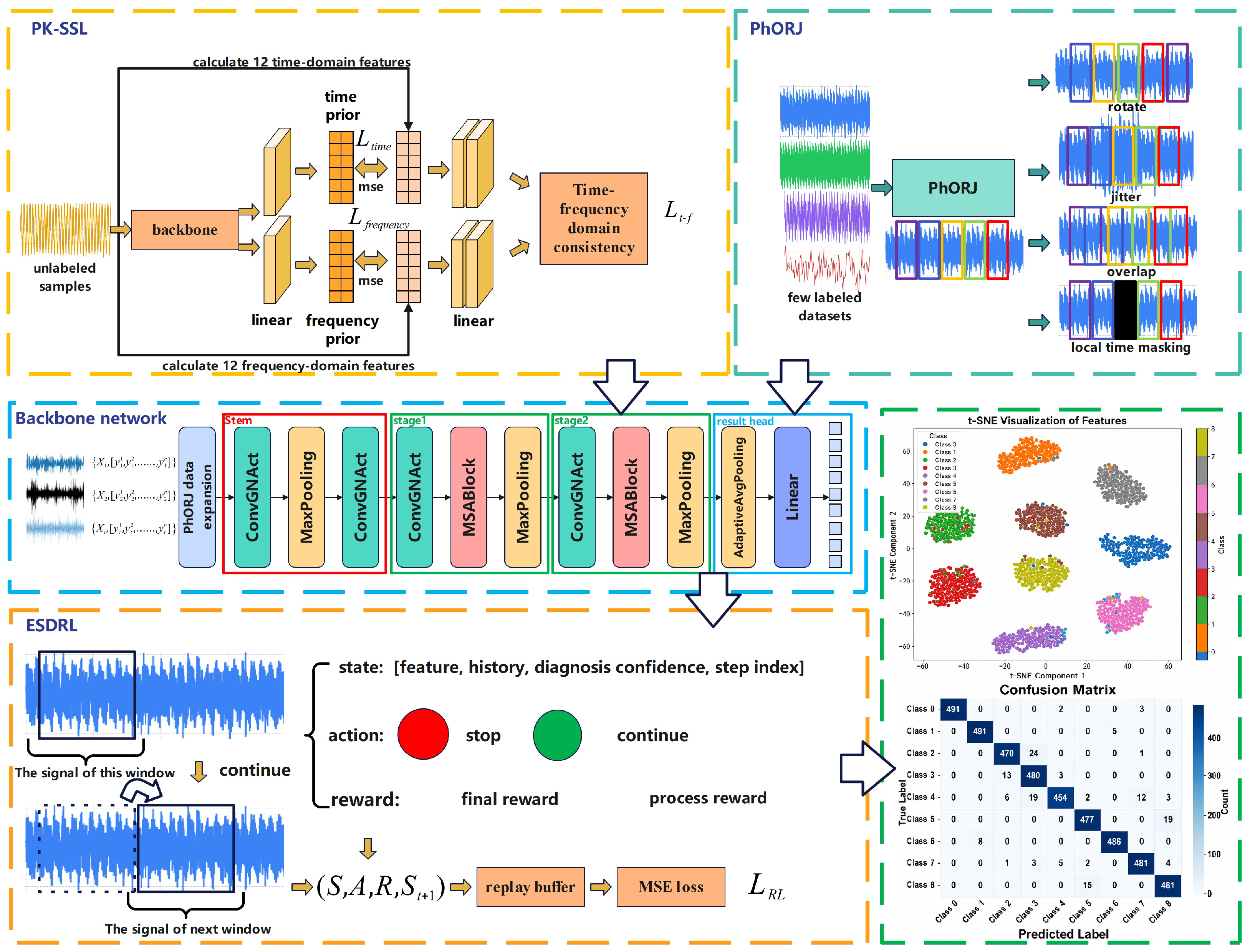
Overall framework of the proposed measurement-efficient few-shot diagnosis system. PK-SSL, PhORJ, and ESDRL are coupled through a shared 1D backbone, so that representation learning, augmentation, and stopping decisions support the same accuracy–measurement–cost objective.
Figure 1.
Overall framework of the proposed measurement-efficient few-shot diagnosis system. PK-SSL, PhORJ, and ESDRL are coupled through a shared 1D backbone, so that representation learning, augmentation, and stopping decisions support the same accuracy–measurement–cost objective.
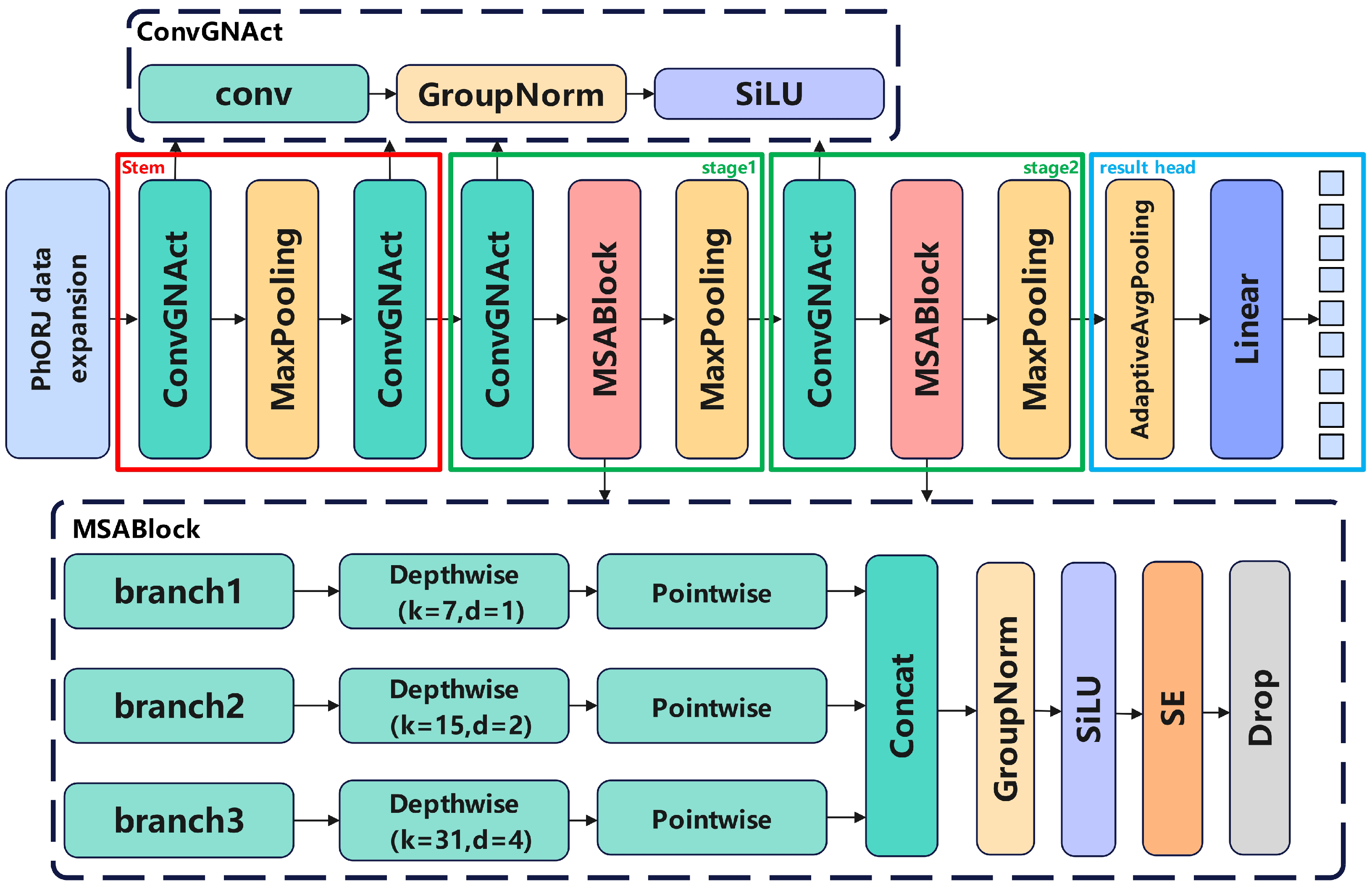
Figure 2.
Architecture of the 1D multi-scale attention backbone. The parallel convolutional branches capture vibration patterns at different temporal scales, and the resulting feature vector is shared by PK-SSL pretraining, few-shot classification, and ESDRL stopping decisions.
Figure 2.
Architecture of the 1D multi-scale attention backbone. The parallel convolutional branches capture vibration patterns at different temporal scales, and the resulting feature vector is shared by PK-SSL pretraining, few-shot classification, and ESDRL stopping decisions.
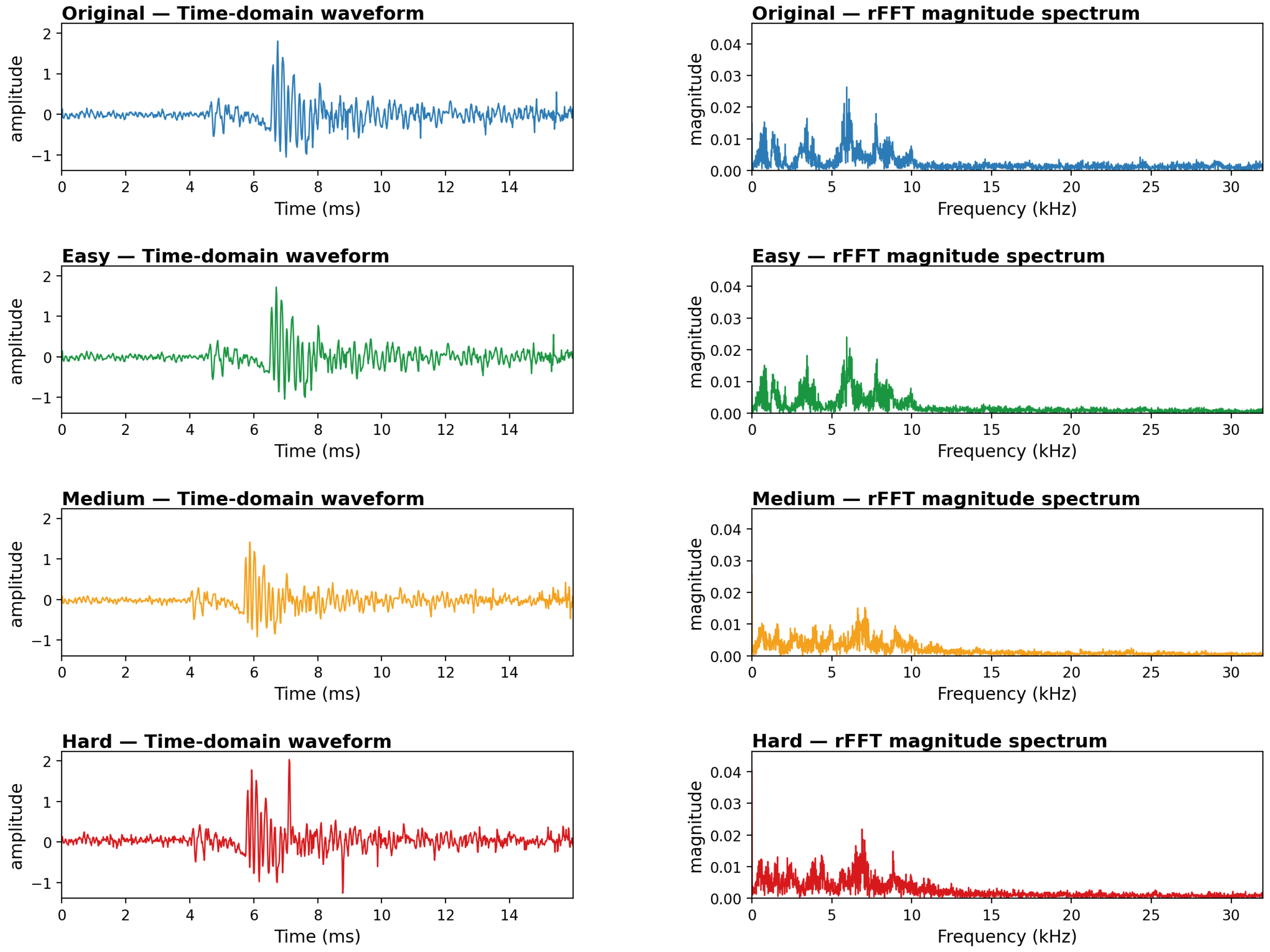
Figure 3.
Representative examples of the four difficulty levels on the same PU bearing sample. Rows correspond to Original, Easy, Medium, and Hard, while the left and right columns show the time-domain waveform and rFFT magnitude spectrum, respectively. From top to bottom, the examples show progressively stronger measurement corruptions, including noise, local information loss, and spectral distortion.
Figure 3.
Representative examples of the four difficulty levels on the same PU bearing sample. Rows correspond to Original, Easy, Medium, and Hard, while the left and right columns show the time-domain waveform and rFFT magnitude spectrum, respectively. From top to bottom, the examples show progressively stronger measurement corruptions, including noise, local information loss, and spectral distortion.
Figure 4.
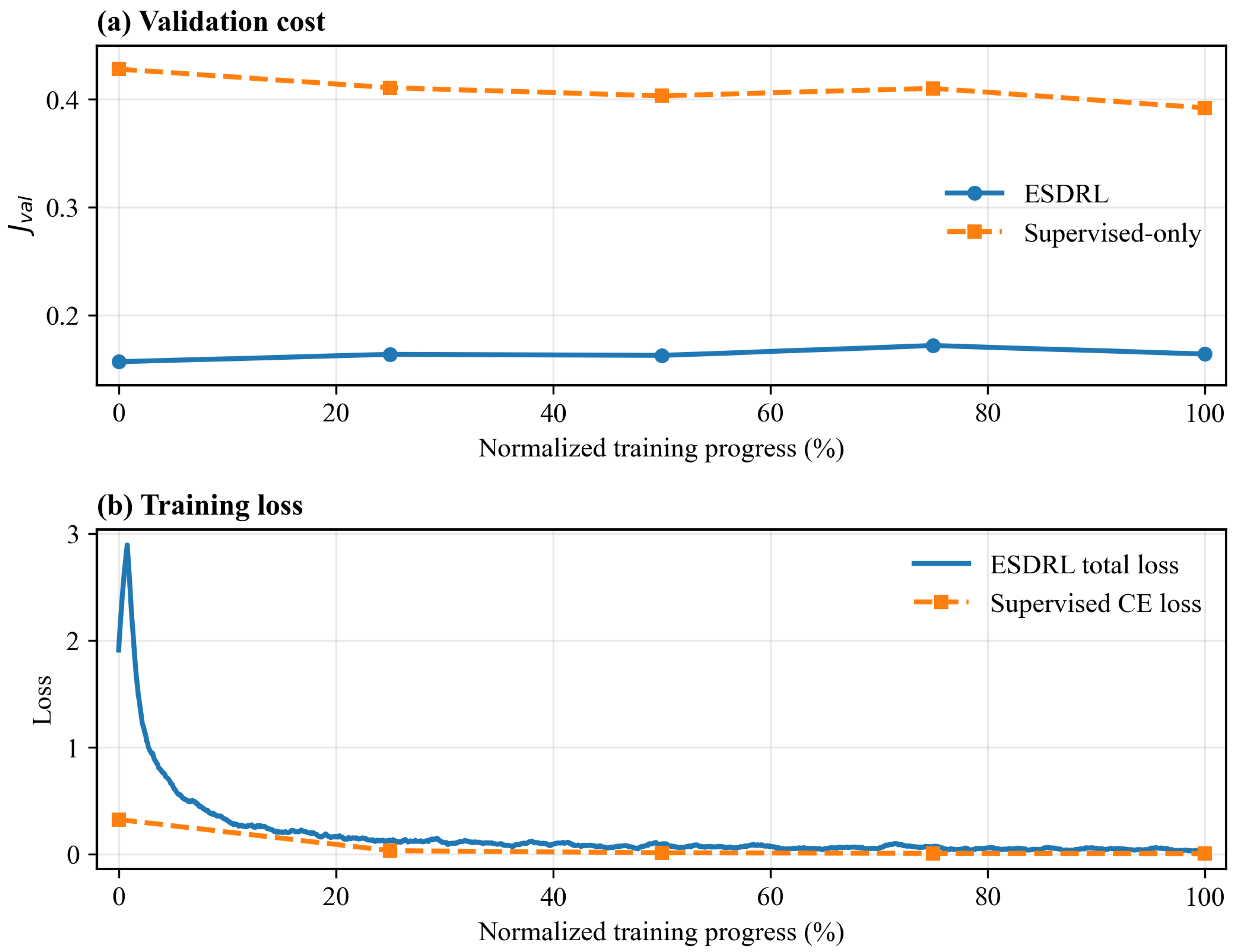
Convergence comparison between the supervised-only training loop and the proposed ESDRL under the representative PU 8-shot setting. (a) Validation cost . (b) Training loss. The supervised-only baseline removes the Double-DQN stopping policy and is trained only with cross-entropy loss. ESDRL uses the joint loss . Lower indicates a better validation accuracy–measurement–cost trade-off.
Figure 4.
Convergence comparison between the supervised-only training loop and the proposed ESDRL under the representative PU 8-shot setting. (a) Validation cost . (b) Training loss. The supervised-only baseline removes the Double-DQN stopping policy and is trained only with cross-entropy loss. ESDRL uses the joint loss . Lower indicates a better validation accuracy–measurement–cost trade-off.
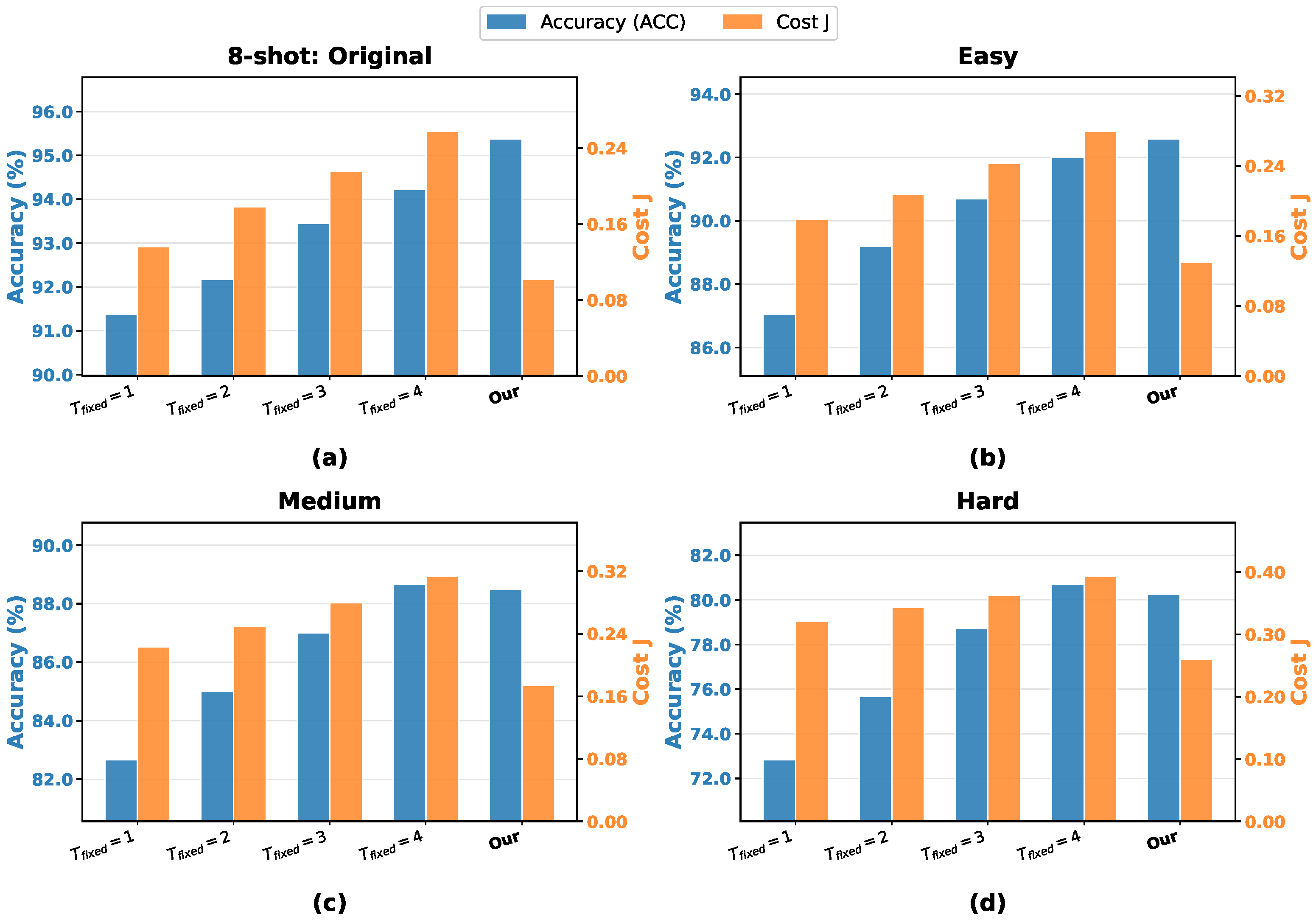
Figure 5.
Accuracy–cost comparison between fixed-window inference and ESDRL on PU under the 8-shot setting. Subfigures (a–d) correspond to Original, Easy, Medium, and Hard, respectively. Blue bars show Accuracy, and orange bars show the evaluation cost J. ESDRL uses an adaptive stopping policy with , while the fixed-window baselines always use or 4 windows.
Figure 5.
Accuracy–cost comparison between fixed-window inference and ESDRL on PU under the 8-shot setting. Subfigures (a–d) correspond to Original, Easy, Medium, and Hard, respectively. Blue bars show Accuracy, and orange bars show the evaluation cost J. ESDRL uses an adaptive stopping policy with , while the fixed-window baselines always use or 4 windows.
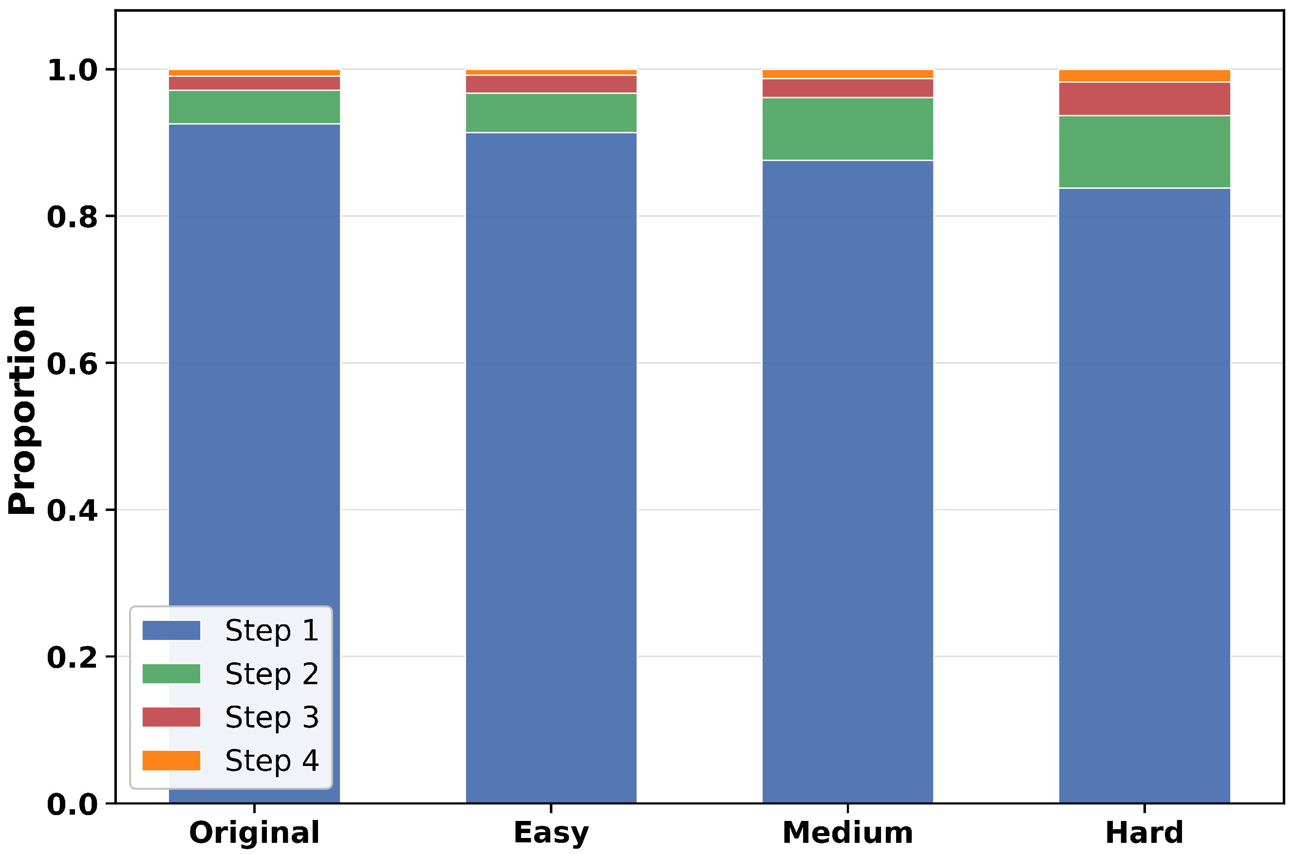
Figure 6.
Stop-at-1/2/3/4 proportions of ESDRL on PU under the 8-shot setting. The four bars correspond to Original, Easy, Medium, and Hard. Harder conditions trigger more step-2/3/4 decisions, showing that the learned policy increases the measurement length when the input is less certain.
Figure 6.
Stop-at-1/2/3/4 proportions of ESDRL on PU under the 8-shot setting. The four bars correspond to Original, Easy, Medium, and Hard. Harder conditions trigger more step-2/3/4 decisions, showing that the learned policy increases the measurement length when the input is less certain.
Figure 7.
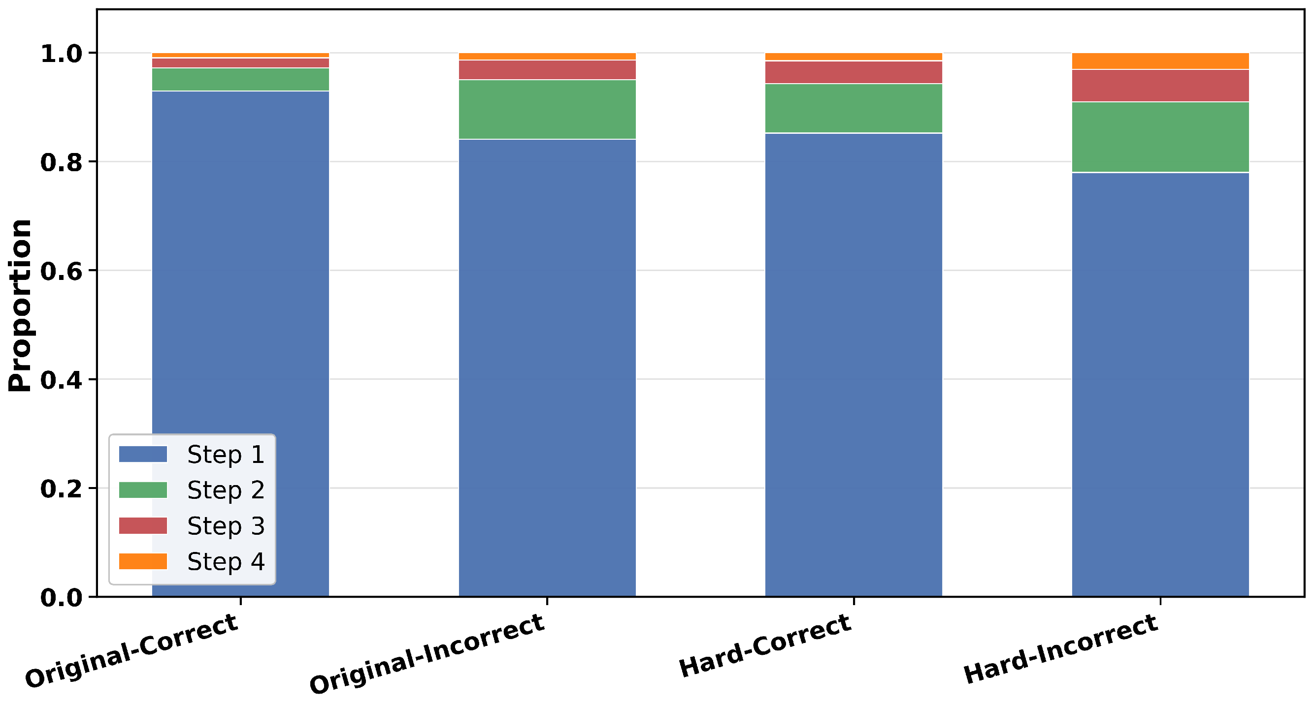
Stopping-step distributions for correctly and incorrectly classified samples on PU under the 8-shot setting. The bars compare Original-correct, Original-incorrect, Hard-correct, and Hard-incorrect samples. Incorrect samples have a larger proportion of later stopping steps, indicating that ambiguous samples tend to consume more measurement budget.
Figure 7.
Stopping-step distributions for correctly and incorrectly classified samples on PU under the 8-shot setting. The bars compare Original-correct, Original-incorrect, Hard-correct, and Hard-incorrect samples. Incorrect samples have a larger proportion of later stopping steps, indicating that ambiguous samples tend to consume more measurement budget.
Figure 8.
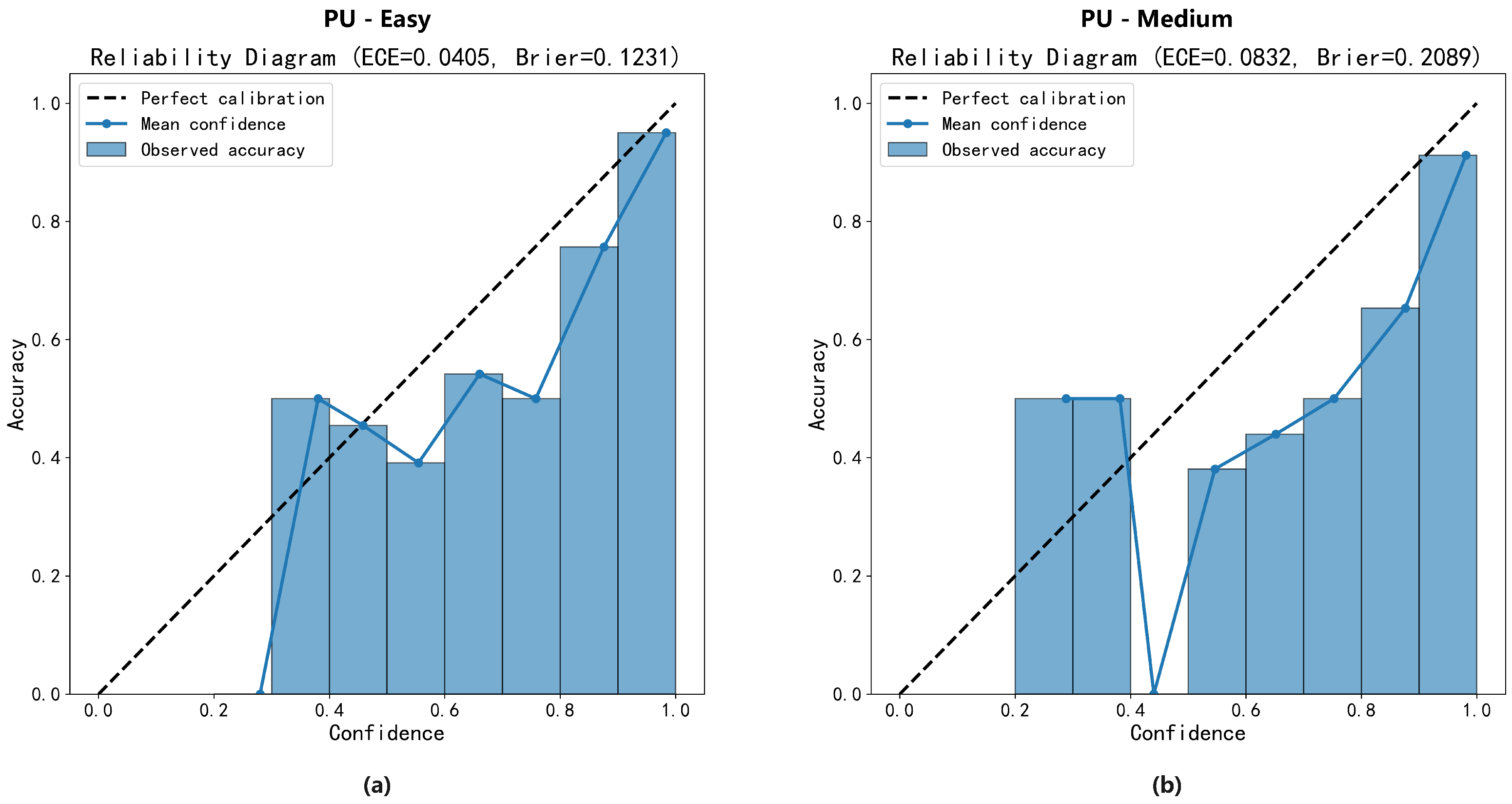
Reliability diagrams of terminal predictions on PU under the 8-shot setting. Subfigures (a,b) correspond to Easy and Medium, respectively. The dashed diagonal line denotes perfect calibration, the blue line shows mean confidence, and the bars show observed accuracy in each confidence bin.
Figure 8.
Reliability diagrams of terminal predictions on PU under the 8-shot setting. Subfigures (a,b) correspond to Easy and Medium, respectively. The dashed diagonal line denotes perfect calibration, the blue line shows mean confidence, and the bars show observed accuracy in each confidence bin.
Figure 9.
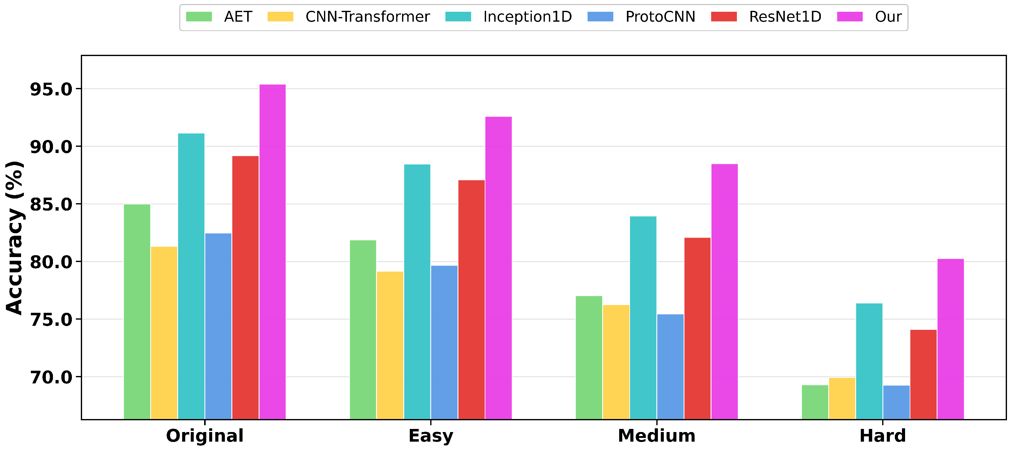
Backbone comparison on PU under the representative 8-shot setting. The x-axis groups the four evaluation difficulty levels: Original, Easy, Medium, and Hard. The y-axis reports classification Accuracy (%). All backbones are trained and evaluated using the same PK-SSL + PhORJ + ESDRL pipeline; only the backbone architecture is changed.
Figure 9.
Backbone comparison on PU under the representative 8-shot setting. The x-axis groups the four evaluation difficulty levels: Original, Easy, Medium, and Hard. The y-axis reports classification Accuracy (%). All backbones are trained and evaluated using the same PK-SSL + PhORJ + ESDRL pipeline; only the backbone architecture is changed.
Figure 10.
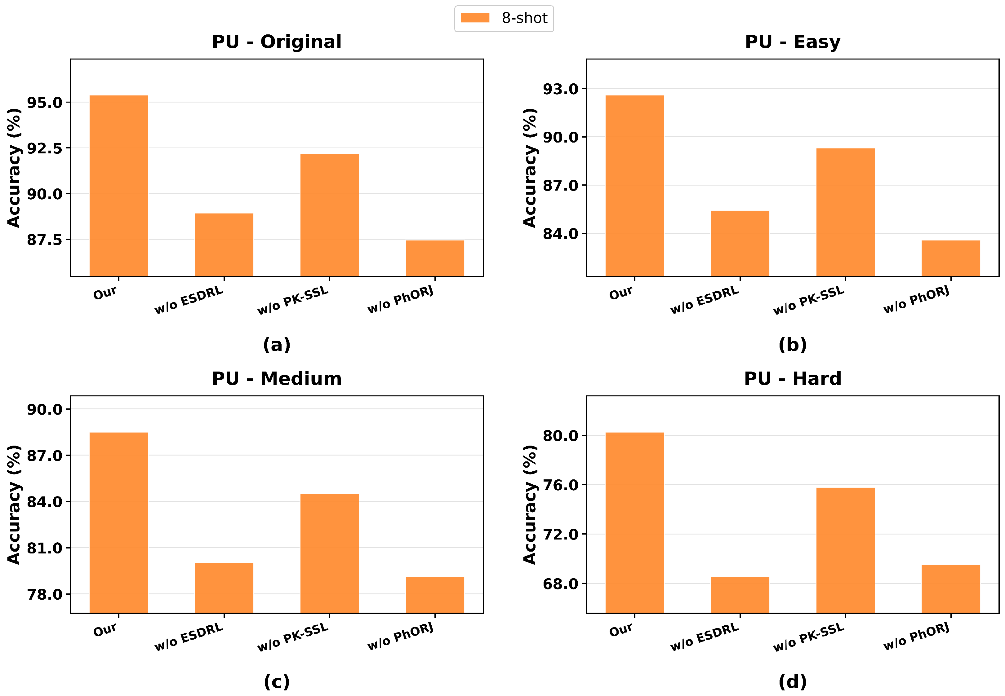
Module-level ablation on PU under the representative 8-shot setting. Subfigures (a–d) correspond to Original, Easy, Medium, and Hard, respectively. Each bar reports classification Accuracy (%). The comparison isolates the contributions of ESDRL, PK-SSL, and PhORJ under the same data split and training protocol.
Figure 10.
Module-level ablation on PU under the representative 8-shot setting. Subfigures (a–d) correspond to Original, Easy, Medium, and Hard, respectively. Each bar reports classification Accuracy (%). The comparison isolates the contributions of ESDRL, PK-SSL, and PhORJ under the same data split and training protocol.
Figure 11.
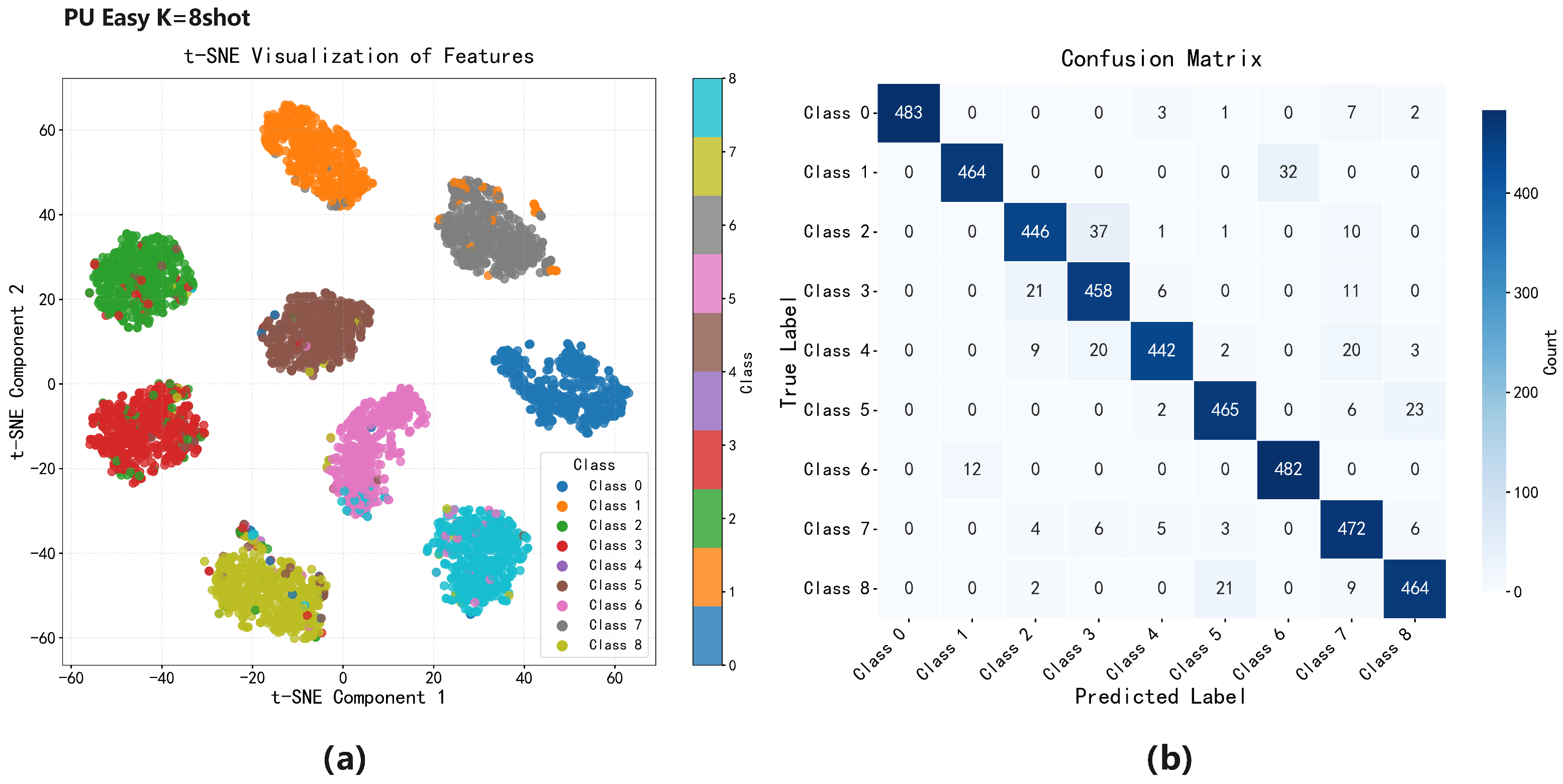
Feature visualization and confusion matrix on PU-Easy under the 8-shot setting. Subfigure (a) shows the t-SNE embedding of the learned features, where colors denote the nine PU classes. Subfigure (b) shows the confusion matrix, where diagonal entries denote correct predictions and off-diagonal entries denote misclassifications.
Figure 11.
Feature visualization and confusion matrix on PU-Easy under the 8-shot setting. Subfigure (a) shows the t-SNE embedding of the learned features, where colors denote the nine PU classes. Subfigure (b) shows the confusion matrix, where diagonal entries denote correct predictions and off-diagonal entries denote misclassifications.
Table 1.
Twelve time-domain prior indicators used in PK-SSL.
Table 1.
Twelve time-domain prior indicators used in PK-SSL.
| Index | Name | Equation |
|---|
| Root mean square (RMS) | |
| Mean value | |
| Standard deviation | |
| Skewness | |
| Kurtosis | |
| Crest factor | |
| Shape factor | |
| Impulse factor | |
| Margin factor | |
| Zero-crossing rate | |
| Peak-to-peak value | |
| Absolute mean value | |
Table 2.
Twelve frequency-domain prior indicators used in PK-SSL.
Table 2.
Twelve frequency-domain prior indicators used in PK-SSL.
| Index | Name | Equation |
|---|
| Main-peak amplitude | |
| Main-peak frequency | |
| Spectral centroid | |
| Spectral spread (2nd central moment) | |
| Band energy 1 (lowest quarter) | |
| Band energy 2 | |
| Band energy 3 | |
| Band energy 4 (highest quarter) | |
| Spectral flatness |
|
| 85% roll-off frequency |
|
| Normalized spectral centroid | |
| High-frequency band energy | |
Table 3.
Data statistics of the UORED-VAFCLS dataset used in the five-class experiment. Base sequences are length- segments extracted by a sliding window with stride .
Table 3.
Data statistics of the UORED-VAFCLS dataset used in the five-class experiment. Base sequences are length- segments extracted by a sliding window with stride .
| Class | Condition | Base Sequences |
|---|
| 1 | Healthy condition | 204 |
| 2 | Inner-race fault | 204 |
| 3 | Outer-race fault | 204 |
| 4 | Ball fault | 204 |
| 5 | Cage fault | 204 |
–Unlabeled healthy base sequences
(for PK-SSL only) | 204 |
Table 4.
Operating conditions and evaluation statistics of the PU dataset (nine-way classification). Base sequences are length- segments extracted by a sliding window with stride .
Table 4.
Operating conditions and evaluation statistics of the PU dataset (nine-way classification). Base sequences are length- segments extracted by a sliding window with stride .
| Class | Operating Condition | Base Sequences |
|---|
| 1 | KA01 (OR, EDM, level 1) | 2470 |
| 2 | KA03 (OR, Electric engraver, level 2) | 2481 |
| 3 | KA05 (OR, Electric engraver, level 1) | 2472 |
| 4 | KA07 (OR, Drilling, level 1) | 2494 |
| 5 | KA08 (OR, Drilling, level 2) | 2471 |
| 6 | KI01 (IR, EDM, level 1) | 2470 |
| 7 | KI03 (IR, Electric engraver, level 1) | 2468 |
| 8 | KI07 (IR, Electric engraver, level 2) | 2481 |
| 9 | K001 (healthy) | 2470 |
–Unlabeled healthy base sequences
(for PK-SSL only) | 2480 |
Table 5.
Parameter ranges used to construct the four difficulty levels. The complexity increases from Easy to Hard through a larger perturbation budget and stronger perturbation ranges.
Table 5.
Parameter ranges used to construct the four difficulty levels. The complexity increases from Easy to Hard through a larger perturbation budget and stronger perturbation ranges.
| Parameter | Original | Easy | Medium | Hard |
|---|
| Additional corruption | None | Yes | Yes | Yes |
| AWGN SNR (dB) | – | 28–32 | 18–22 | 10–14 |
| Impulse count per corrupted window | – | 0–2 | 2–4 | 4–6 |
| Impulse amplitude () | – | 2.0–3.0 | 3.0–4.0 | 4.0–6.0 |
| Notch bandwidth | – | 0.02–0.05 | 0.05–0.10 | 0.08–0.15 |
| Time-warp strength | – | 0.00–0.02 | 0.02–0.05 | 0.05–0.08 |
| Time-mask ratio | – | 0.02–0.05 | 0.05–0.10 | 0.10–0.15 |
| Amplitude scaling | – | 0.90–1.10 | 0.85–1.15 | 0.80–1.20 |
| Bias drift (×RMS) | – | 0.05–0.10 | 0.10–0.20 | 0.20–0.30 |
| Maximum circular shift (samples) | – | 16–32 | 32–64 | 64–128 |
| Operations per corrupted window | 0 | 1 | 1–2 | 2–3 |
| Narrow-band noise center | 0.05–0.45, used only when narrow-band noise is selected |
| Narrow-band noise bandwidth | 0.01–0.05, used only when narrow-band noise is selected |
| Narrow-band noise amplitude | 0.2–0.6 × RMS, used only when narrow-band noise is selected |
| Corruption templates | T1–T6 over four measurement steps; see note below |
Table 6.
Key hyperparameters for Double-DQN training in ESDRL.
Table 6.
Key hyperparameters for Double-DQN training in ESDRL.
| Hyperparameter | Value | Unit/Meaning |
|---|
| Replay buffer capacity | 5000 | transitions |
| Warm-up before updates | 2000 | transitions |
| Mini-batch size B | 64 | transitions/update |
| Maximum horizon | 4 | decision steps |
| Discount factor | 0.90 | dimensionless |
| DRL loss | Huber | TD loss |
| Target-network update | 0.005 | soft-update factor |
| Exploration | -greedy | action exploration |
| Optimizer | Adam | optimizer type |
| Learning rate | | dimensionless |
| Gradient clipping | 1.0 | global norm |
| Step cost | 0.05 | reward cost/step |
| RL loss weight | 0.10 | dimensionless |
Table 7.
Compact fairness protocol for baseline comparison. Under the same random seed and the same K-shot setting, all methods use the same raw-record split, the same K-shot support set, and the same evaluation subsets.
Table 7.
Compact fairness protocol for baseline comparison. Under the same random seed and the same K-shot setting, all methods use the same raw-record split, the same K-shot support set, and the same evaluation subsets.
| Method Group | Extra Training Information | Inference Protocol |
|---|
| CNN baselines | Same K-shot support set only; no PhORJ and no PK-SSL | Fixed-window classification |
| ProtoNet + PhORJ | Same support set with PhORJ augmentation under the same augmentation budget; no PK-SSL | Static prototype classification |
| CTQN | Same K-shot support set; no PhORJ and no PK-SSL | Fixed-horizon Q-value aggregation with |
| Ours | Same K-shot support set with PhORJ; PK-SSL uses a separate healthy-only unlabeled pool without fault labels | Adaptive STOP/CONTINUE stopping with maximum horizon |
Table 8.
Few-shot results on UORED-VAFCLS under : Accuracy and AUC. Each cell reports Accuracy ± standard deviation/Macro-AUC (%).
Table 8.
Few-shot results on UORED-VAFCLS under : Accuracy and AUC. Each cell reports Accuracy ± standard deviation/Macro-AUC (%).
| Method | Diff. | 6-Shot Acc./AUC | 8-Shot Acc./AUC | 10-Shot Acc./AUC |
|---|
| MSFFNET | Original | | | |
| MSFFNET | Easy | | | |
| MSFFNET | Medium | | | |
| MSFFNET | Hard | | | |
| MSCNN | Original | | | |
| MSCNN | Easy | | | |
| MSCNN | Medium | | | |
| MSCNN | Hard | | | |
| WDCNN | Original | | | |
| WDCNN | Easy | | | |
| WDCNN | Medium | | | |
| WDCNN | Hard | | | |
| MSAFCN | Original | | | |
| MSAFCN | Easy | | | |
| MSAFCN | Medium | | | |
| MSAFCN | Hard | | | |
| ProtoNet + PhORJ | Original | | | |
| ProtoNet + PhORJ | Easy | | | |
| ProtoNet + PhORJ | Medium | | | |
| ProtoNet + PhORJ | Hard | | | |
| CTQN | Original | | | |
| CTQN | Easy | | | |
| CTQN | Medium | | | |
| CTQN | Hard | | | |
| Ours | Original | | | |
| Ours | Easy | | | |
| Ours | Medium | | | |
| Ours | Hard | | | |
Table 9.
Few-shot results on UORED-VAFCLS under : Macro-Precision, Macro-Recall and Macro-F1. Each cell reports Macro-Precision/Macro-Recall/Macro-F1 (%).
Table 9.
Few-shot results on UORED-VAFCLS under : Macro-Precision, Macro-Recall and Macro-F1. Each cell reports Macro-Precision/Macro-Recall/Macro-F1 (%).
| Method | Diff. | 6-Shot P/R/F1 | 8-Shot P/R/F1 | 10-Shot P/R/F1 |
|---|
| MSFFNET | Original | | | |
| MSFFNET | Easy | | | |
| MSFFNET | Medium | | | |
| MSFFNET | Hard | | | |
| MSCNN | Original | | | |
| MSCNN | Easy | | | |
| MSCNN | Medium | | | |
| MSCNN | Hard | | | |
| WDCNN | Original | | | |
| WDCNN | Easy | | | |
| WDCNN | Medium | | | |
| WDCNN | Hard | | | |
| MSAFCN | Original | | | |
| MSAFCN | Easy | | | |
| MSAFCN | Medium | | | |
| MSAFCN | Hard | | | |
| ProtoNet + PhORJ | Original | | | |
| ProtoNet + PhORJ | Easy | | | |
| ProtoNet + PhORJ | Medium | | | |
| ProtoNet + PhORJ | Hard | | | |
| CTQN | Original | | | |
| CTQN | Easy | | | |
| CTQN | Medium | | | |
| CTQN | Hard | | | |
| Ours | Original | | | |
| Ours | Easy | | | |
| Ours | Medium | | | |
| Ours | Hard | | | |
Table 10.
Few-shot results on the PU dataset under : Accuracy and AUC. Each cell reports Accuracy ± standard deviation/Macro-AUC (%).
Table 10.
Few-shot results on the PU dataset under : Accuracy and AUC. Each cell reports Accuracy ± standard deviation/Macro-AUC (%).
| Method | Diff. | 6-Shot Acc./AUC | 8-Shot Acc./AUC | 10-Shot Acc./AUC |
|---|
| MSFFNET | Original | | | |
| MSFFNET | Easy | | | |
| MSFFNET | Medium | | | |
| MSFFNET | Hard | | | |
| MSCNN | Original | | | |
| MSCNN | Easy | | | |
| MSCNN | Medium | | | |
| MSCNN | Hard | | | |
| WDCNN | Original | | | |
| WDCNN | Easy | | | |
| WDCNN | Medium | | | |
| WDCNN | Hard | | | |
| MSAFCN | Original | | | |
| MSAFCN | Easy | | | |
| MSAFCN | Medium | | | |
| MSAFCN | Hard | | | |
| ProtoNet + PhORJ | Original | | | |
| ProtoNet + PhORJ | Easy | | | |
| ProtoNet + PhORJ | Medium | | | |
| ProtoNet + PhORJ | Hard | | | |
| CTQN | Original | | | |
| CTQN | Easy | | | |
| CTQN | Medium | | | |
| CTQN | Hard | | | |
| Ours | Original | | | |
| Ours | Easy | | | |
| Ours | Medium | | | |
| Ours | Hard | | | |
Table 11.
Few-shot results on the PU dataset under : Macro-Precision, Macro-Recall and Macro-F1. Each cell reports Macro-Precision/Macro-Recall/Macro-F1 (%).
Table 11.
Few-shot results on the PU dataset under : Macro-Precision, Macro-Recall and Macro-F1. Each cell reports Macro-Precision/Macro-Recall/Macro-F1 (%).
| Method | Diff. | 6-Shot P/R/F1 | 8-Shot P/R/F1 | 10-Shot P/R/F1 |
|---|
| MSFFNET | Original | | | |
| MSFFNET | Easy | | | |
| MSFFNET | Medium | | | |
| MSFFNET | Hard | | | |
| MSCNN | Original | | | |
| MSCNN | Easy | | | |
| MSCNN | Medium | | | |
| MSCNN | Hard | | | |
| WDCNN | Original | | | |
| WDCNN | Easy | | | |
| WDCNN | Medium | | | |
| WDCNN | Hard | | | |
| MSAFCN | Original | | | |
| MSAFCN | Easy | | | |
| MSAFCN | Medium | | | |
| MSAFCN | Hard | | | |
| ProtoNet + PhORJ | Original | | | |
| ProtoNet + PhORJ | Easy | | | |
| ProtoNet + PhORJ | Medium | | | |
| ProtoNet + PhORJ | Hard | | | |
| CTQN | Original | | | |
| CTQN | Easy | | | |
| CTQN | Medium | | | |
| CTQN | Hard | | | |
| Ours | Original | | | |
| Ours | Easy | | | |
| Ours | Medium | | | |
| Ours | Hard | | | |
Table 12.
Robustness to mislabeled support samples on PU under the 8-shot setting: Accuracy and AUC. Each cell reports Accuracy ± standard deviation/Macro-AUC (%).
Table 12.
Robustness to mislabeled support samples on PU under the 8-shot setting: Accuracy and AUC. Each cell reports Accuracy ± standard deviation/Macro-AUC (%).
| Method | Diff. | 0% Acc./AUC | 10% Acc./AUC | 20% Acc./AUC |
|---|
| WDCNN | Original | | | |
| ProtoNet + PhORJ | Original | | | |
| CTQN | Original | | | |
| Ours | Original | | | |
| WDCNN | Easy | | | |
| ProtoNet + PhORJ | Easy | | | |
| CTQN | Easy | | | |
| Ours | Easy | | | |
| WDCNN | Medium | | | |
| ProtoNet + PhORJ | Medium | | | |
| CTQN | Medium | | | |
| Ours | Medium | | | |
| WDCNN | Hard | | | |
| ProtoNet + PhORJ | Hard | | | |
| CTQN | Hard | | | |
| Ours | Hard | | | |
Table 13.
Robustness to mislabeled support samples on PU under the 8-shot setting: Macro-Precision, Macro-Recall and Macro-F1. Each cell reports Macro-Precision/Macro-Recall/Macro-F1 (%).
Table 13.
Robustness to mislabeled support samples on PU under the 8-shot setting: Macro-Precision, Macro-Recall and Macro-F1. Each cell reports Macro-Precision/Macro-Recall/Macro-F1 (%).
| Method | Diff. | 0% P/R/F1 | 10% P/R/F1 | 20% P/R/F1 |
|---|
| WDCNN | Original | | | |
| ProtoNet + PhORJ | Original | | | |
| CTQN | Original | | | |
| Ours | Original | | | |
| WDCNN | Easy | | | |
| ProtoNet + PhORJ | Easy | | | |
| CTQN | Easy | | | |
| Ours | Easy | | | |
| WDCNN | Medium | | | |
| ProtoNet + PhORJ | Medium | | | |
| CTQN | Medium | | | |
| Ours | Medium | | | |
| WDCNN | Hard | | | |
| ProtoNet + PhORJ | Hard | | | |
| CTQN | Hard | | | |
| Ours | Hard | | | |
Table 14.
Average stopping step of ESDRL on PU across shot settings and difficulty levels. Larger values indicate that the policy acquires more windows before stopping.
Table 14.
Average stopping step of ESDRL on PU across shot settings and difficulty levels. Larger values indicate that the policy acquires more windows before stopping.
| Shot Setting | Original | Easy | Medium | Hard |
|---|
| 6-shot | 1.1343 | 1.1692 | 1.2047 | 1.2717 |
| 8-shot | 1.1132 | 1.1275 | 1.1762 | 1.2432 |
| 10-shot | 1.1098 | 1.1260 | 1.1645 | 1.2289 |
Table 15.
Online inference efficiency of different stopping strategies on PU under the 8-shot setting. All strategies use the same backbone and differ only in the stopping rule. Here denotes the average number of acquired windows, and indicates that a lower J value is better.
Table 15.
Online inference efficiency of different stopping strategies on PU under the 8-shot setting. All strategies use the same backbone and differ only in the stopping rule. Here denotes the average number of acquired windows, and indicates that a lower J value is better.
| Difficulty | Strategy | Acc. (%) | Avg. Windows | Latency/Sample (ms) | |
|---|
| Original | Fixed | | 1.000 | 1.685 | 0.1363 |
| Original | Fixed | | 2.000 | 3.352 | 0.1783 |
| Original | Fixed | | 3.000 | 5.125 | 0.2155 |
| Original | Fixed | | 4.000 | 6.360 | 0.2578 |
| Original | Confidence threshold | | 1.155 | 1.820 | 0.1218 |
| Original | ESDRL (Ours) | | 1.1132 | 1.848 | 0.1019 |
| Easy | Fixed | | 1.000 | 1.642 | 0.1796 |
| Easy | Fixed | | 2.000 | 3.344 | 0.2081 |
| Easy | Fixed | | 3.000 | 4.788 | 0.2431 |
| Easy | Fixed | | 4.000 | 6.717 | 0.2800 |
| Easy | Confidence threshold | | 1.185 | 1.851 | 0.1593 |
| Easy | ESDRL (Ours) | | 1.1275 | 1.949 | 0.1305 |
| Medium | Fixed | | 1.000 | 1.633 | 0.2234 |
| Medium | Fixed | | 2.000 | 3.392 | 0.2499 |
| Medium | Fixed | | 3.000 | 4.845 | 0.2799 |
| Medium | Fixed | | 4.000 | 6.700 | 0.3133 |
| Medium | Confidence threshold | | 1.244 | 1.906 | 0.2030 |
| Medium | ESDRL (Ours) | | 1.1762 | 1.933 | 0.1738 |
| Hard | Fixed | | 1.000 | 1.726 | 0.3217 |
| Hard | Fixed | | 2.000 | 3.436 | 0.3432 |
| Hard | Fixed | | 3.000 | 4.777 | 0.3626 |
| Hard | Fixed | | 4.000 | 6.760 | 0.3929 |
| Hard | Confidence threshold | | 1.311 | 1.921 | 0.2773 |
| Hard | ESDRL (Ours) | | 1.2432 | 1.976 | 0.2596 |
Table 16.
Static computational complexity of representative methods for one 1024-point input window. Ours is heavier than MSCNN per window, but ESDRL usually evaluates far fewer windows per sample, as shown in
Table 15.
Table 16.
Static computational complexity of representative methods for one 1024-point input window. Ours is heavier than MSCNN per window, but ESDRL usually evaluates far fewer windows per sample, as shown in
Table 15.
| Method | Params (M) | MACs (M) | Latency/Window (ms) | Throughput (Windows/s) |
|---|
| MSCNN | 0.035 | 8.05 | 0.435 | 2299.8 |
| CTQN | 0.530 | 16.25 | 1.049 | 953.2 |
| Ours | 0.276 | 53.96 | 1.632 | 612.6 |
Table 17.
Calibration metrics of terminal predictions on PU under the 8-shot setting. Lower ECE and Brier scores indicate better calibrated confidence.
Table 17.
Calibration metrics of terminal predictions on PU under the 8-shot setting. Lower ECE and Brier scores indicate better calibrated confidence.
| Setting | ECE | Brier Score |
|---|
| PU-Original | 0.0162 | 0.0711 |
| PU-Easy | 0.0405 | 0.1231 |
| PU-Medium | 0.0832 | 0.2089 |
| PU-Hard | 0.1509 | 0.3534 |
Table 18.
Fine-grained ablation of PK-SSL on PU under the representative 8-shot setting. Results are reported as mean ± standard deviation.
Table 18.
Fine-grained ablation of PK-SSL on PU under the representative 8-shot setting. Results are reported as mean ± standard deviation.
| Pretraining Strategy | Original | Easy | Medium | Hard |
|---|
| No pretraining | | | | |
| Generic SSL pretraining | | | | |
| Time-only PK-SSL | | | | |
| Frequency-only PK-SSL | | | | |
| Time + Freq w/o consistency | | | | |
| Full PK-SSL | | | | |
Table 19.
Fine-grained ablation of PhORJ on PU under the representative 8-shot setting. Results are reported as mean ± standard deviation.
Table 19.
Fine-grained ablation of PhORJ on PU under the representative 8-shot setting. Results are reported as mean ± standard deviation.
| Augmentation Variant | Original | Easy | Medium | Hard |
|---|
| Classical ORJ | | | | |
| PhORJ w/o band ops | | | | |
| PhORJ w/o phase jitter | | | | |
| PhORJ w/o global time warp | | | | |
| PhORJ w/o local time masking | | | | |
| Full PhORJ | | | | |
Table 20.
Compact sensitivity summary of the main ESDRL-related coefficients on PU under the representative 8-shot setting. For each parameter value, we report the average accuracy, average stopping step , and average cost J over the four difficulty levels.
Table 20.
Compact sensitivity summary of the main ESDRL-related coefficients on PU under the representative 8-shot setting. For each parameter value, we report the average accuracy, average stopping step , and average cost J over the four difficulty levels.
| Parameter | Value | Avg. Acc. (%) | Avg. Step | Avg. J |
|---|
| 0.01 | 88.37 | 1.2192 | 0.1773 |
| 0.03 | 88.61 | 1.1735 | 0.1726 |
| 0.05 | 89.18 | 1.1650 | 0.1664 |
| 0.07 | 88.14 | 1.1978 | 0.1785 |
| 0.10 | 88.41 | 1.1853 | 0.1751 |
| 0.05 | 88.19 | 1.1808 | 0.1771 |
| 0.10 | 89.18 | 1.1650 | 0.1664 |
| 0.20 | 88.35 | 1.1803 | 0.1755 |
| 0.50 | 88.04 | 1.2240 | 0.1808 |
| 0.50 | 88.58 | 1.1727 | 0.1729 |
| 0.70 | 88.63 | 1.1717 | 0.1723 |
| 0.90 | 89.18 | 1.1650 | 0.1664 |
| 0.99 | 88.48 | 1.2065 | 0.1755 |



 ,
,