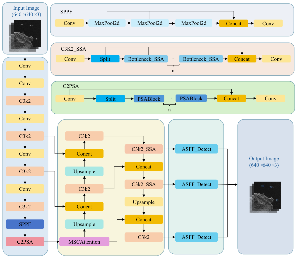
Figure 1 gives an overview of the MSA-DET architecture. The detector builds on YOLOv11 and introduces three coordinated modifications, each targeting a different bottleneck in SAR ship detection. All three modules draw on existing techniques that are adapted to the SAR context in specific ways: MSCAttention is originally proposed for medical image segmentation [
29] and is here repurposed for SAR by placing it at the deepest backbone stage (after Stage 4) where receptive-field diversity is most needed for multi-scale ship echoes; C3k2_SSA adapts the SparseViT attention [
30] from image manipulation localization into a CSP bottleneck, exploiting its sparsification property specifically to zero-weight speckle-dominated background tokens; and ASFF [
27] is applied here to replace the YOLOv11 detection head with learnable per-pixel fusion weights, addressing the scale inconsistency problem that is particularly pronounced in SAR harbor scenes. The modifications are described below, with explicit comparison to the original published implementations where relevant.
These three modifications work as an integrated whole rather than independent add-ons. The sections that follow describe the design rationale behind each module in detail; comparative and ablation experiments then quantify both the individual and combined effects of these components.
3.1. MSCAttention Module
Standard self-attention captures global context but scales quadratically,
, a cost that becomes prohibitive on high-resolution SAR feature maps [
42,
43]. Axial Attention brings this down to
by decomposing 2D attention into successive horizontal and vertical passes [
43]. The sequential nature of that decomposition, though, limits how much the two spatial dimensions can interact with each other. Most existing attention designs also process features at a single scale [
42,
44]—a poor match for SAR images where ship targets range from small fishing boats to large cargo vessels within the same scene.
We address both shortcomings by adapting the cross-axis attention mechanism from MCANet [
29] into the SAR detection backbone. MCANet’s decode head attention runs two axial branches in parallel—each aggregating multi-scale 1D strip features along one axis—and couples them cross-dimensionally by routing each branch’s queries from the opposite axis’s feature map. The kernel configuration (1 × 7, 1 × 11, 1 × 21 horizontal and their vertical counterparts), the depthwise-separable grouping, and the cross-axis Q-K-V coupling are inherited directly from that design. Our contribution is the domain transfer: transplanting this mechanism from a medical image segmentation decoder, where it was designed for pixel-level boundary discrimination, to the deepest stage of a SAR object detection backbone, where its multi-scale receptive fields and bidirectional spatial coupling address the scale and orientation diversity of ship echoes in cluttered SAR scenes. MSCAttention is inserted at Layer 11, after the backbone has applied five stride-2 downsampling operations that reduce the
input to a
feature map (1/32 of the input resolution); operating at this compressed spatial scale keeps the attention overhead modest while allowing the module to capture global ship-level context.
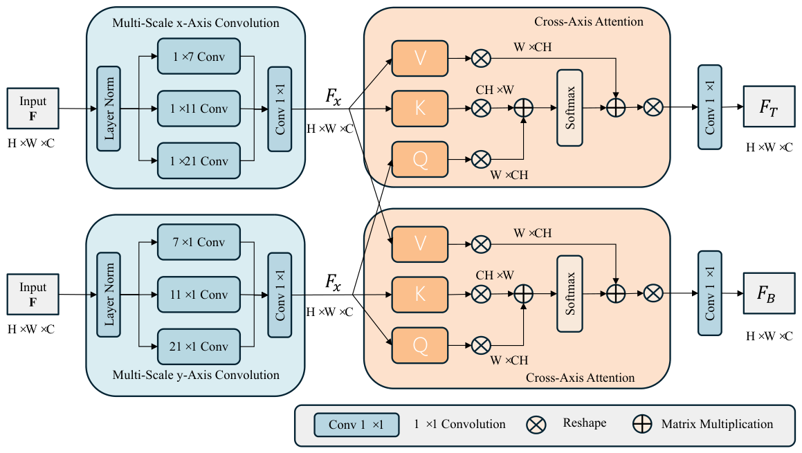
The internal structure is shown in
Figure 2. Given an input feature map
(where
H and
W are the spatial height and width of the feature map in pixels, and
C is the number of channels), the module splits processing into an
x-axis branch and a
y-axis branch. Each branch applies three 1D convolution kernels of different sizes (
x-axis:
,
,
;
y-axis:
,
,
) to the layer-normalized input. The three kernel sizes are chosen to cover three distinct receptive-field regimes on the
feature map (1/32 of the input resolution): 7-pixel kernels target short-range context corresponding to small vessels, 11-pixel kernels capture mid-range context for medium-sized ships, and 21-pixel kernels provide long-range context for large targets; together they span the full scale range of SAR ship echoes observed in HRSID and SSDD without requiring separate branches per target category. In the
x-axis branch the multi-scale outputs are summed and compressed through a
convolution:
The
y-axis branch produces
in a mirror fashion. Cross-axis attention is then constructed as follows. For the horizontal branch, Keys (
K) and Values (
V) come from
while Queries (
Q) come from
; dot-product similarity is computed, normalized with Softmax, and used to weight
V. A residual connection yields the horizontal cross-axis feature
. The vertical branch reverses the roles:
Q is drawn from
, and
from
, producing
. Eight attention heads operate in parallel to widen the representational capacity. Because each branch’s queries originate in the opposite axis, the module captures global dependencies along both directions simultaneously—something sequential axial attention cannot achieve. The final output folds the two refined branches back together with the original input through a residual path:
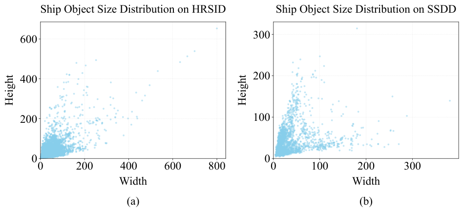
The three kernel widths—7, 11, and 21 pixels—are chosen to span the typical spatial extent of SAR ship targets: short-range (7-pixel) kernels capture fine structural details such as superstructure edges, medium-range (11-pixel) kernels cover the body width of small-to-medium vessels, and long-range (21-pixel) kernels address the full length of large cargo ships. These scales align with the bounding-box size distribution observed in HRSID, where ship lengths range roughly from 10 to 200 pixels at the native
resolution. The number of attention heads is set to
following standard transformer practice [
45]: with
channels per head, each head captures a distinct subspace of the joint spatial representation, and 8 heads provide a good balance between representational diversity and computational efficiency.
Within MSA-DET, MSCAttention is placed at Layer 11—after the SPPF layer (Layer 9) and C2PSA block (Layer 10) at the deepest backbone stage. The YOLOv11 backbone applies five stride-2 downsampling steps (Layers 0, 1, 3, 5, and 7), so Layer 11 operates on feature maps ( of the input). At this compact resolution the computational overhead of multi-scale cross-axis attention is modest, while the rich semantics of deep features and the large effective receptive fields are precisely what is needed to discriminate ship echoes from complex sea clutter.
3.2. C3k2_SSA Module
How well a detector extracts features largely determines its final accuracy. Conventional CNNs such as ResNet [
46] are adept at encoding local texture, yet their fixed-geometry kernels cap the effective receptive field, leaving long-range spatial relationships under-represented. Vision Transformers (ViT) [
47] remedy this through self-attention over the full feature map, but at
cost—impractical once resolution climbs. Window-based variants like Swin Transformer [
48] cut that cost by confining attention to local patches, though stitching information across windows adds its own design overhead.
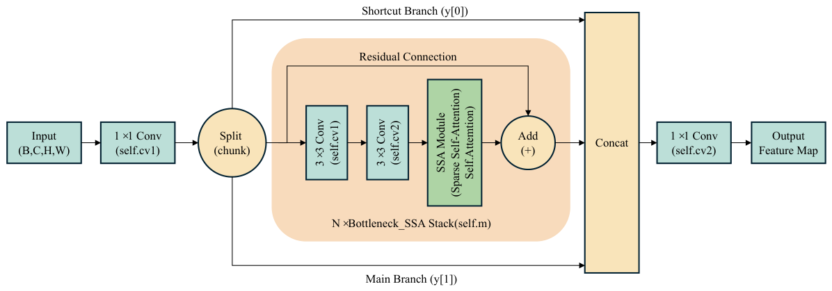
We seek a middle ground: global context at sub-quadratic expense. To that end, the Sparse Self-Attention (SSA) block of Su et al. [
30] is integrated into the C3k2 CSP bottleneck, yielding the C3k2_SSA module depicted in
Figure 3. The SSA block itself retains its original design from SparseViT [
30]: layer-scale parameters initialized at
for training stability, a depthwise convolutional positional embedding (
,
groups=dim), and fused linear projections for Q, K, and V. The contribution of C3k2_SSA is the integration strategy: SSA is appended to the two-convolution path of a C3k2 CSP bottleneck, creating a serial CNN-then-attention block that first extracts local texture with standard convolutions before applying sparse global attention. This hybrid is then selectively deployed at the P3 and P4 neck levels, while P5 retains a standard C3k2 block—a deliberate choice that concentrates sparse attention at the feature scales where small and medium ship discrimination is most critical.
The key idea is to let self-attention operate only on the most informative token pairs. For an input feature map
(notation consistent with
Section 3.1;
denotes the total number of spatial tokens), linear projections first produce the familiar Query (
Q), Key (
K), and Value (
V) matrices:
where
are learnable projection matrices and
is the per-head dimension (
h denotes the number of attention heads, set to 4 following the default configuration of the original SSA implementation [
30]). Whereas standard attention computes dense pairwise scores, SSA applies a Top-
k sparsification with
(retaining the top 25% of key positions per query, following [
30]): for every query position
i, only the
k highest-scoring key positions
j are retained; all other entries are masked to
, effectively zeroing their contribution after Softmax. The resulting sparse attention matrix
M takes the form
Here
collects all raw attention scores for the
i-th query before sparsification. The attended output follows the usual weighted aggregation
A residual connection then merges
with the original input, preserving gradient flow and encouraging feature reuse. The net effect resembles a selective filter: the network attends to the few most relevant spatial locations—typically ship pixels and their immediate surroundings—while background clutter and speckle receive near-zero weight.
Inside MSA-DET, C3k2_SSA blocks are deployed at three neck positions: Layer 14 (, after concatenation with backbone features), Layer 17 (, for small-target detection), and Layer 20 (, after bottom-up path aggregation). Layer 23 (, large-vessel scale) retains a standard C3k2 block, because large ships produce high-confidence detections even without sparse attention, and allocating SSA computation to the coarsest level yields diminishing returns. This selective deployment concentrates sparse attention where small and medium ship discrimination is most challenging, while keeping the overall FLOPs increase moderate.
3.3. ASFF-Head Module
Single-stage detectors built on feature pyramids usually merge information across scales with element-wise addition or simple concatenation [
25,
49]. Neither operation accounts for a fundamental mismatch: a ship that serves as a positive training sample at one pyramid level may overlap with pure background at another, creating gradient conflicts that confuse the optimizer [
50]. Some work sidesteps this by masking out nearby-level regions [
51], but such hand-crafted rules tend to produce false alarms at whichever level was suppressed. A more principled solution is to let the network decide, at every spatial position, how much each level should contribute. That is precisely what the Adaptive Spatial Feature Fusion (ASFF) detection head [
27] does—it learns per-pixel fusion weights that filter out conflicting signals, with negligible extra latency.
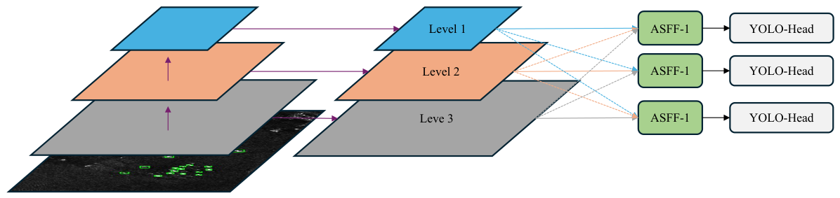
The mechanism operates as follows (see
Figure 4). Three feature maps from the neck (Levels 1–3) are first aligned to a common spatial resolution: for a target level
l, every other level’s features
are resized through upsampling or downsampling to yield
. Fusion then proceeds through learned spatial weights. Taking Level 1 as an illustration, the output at each position is
where
are non-negative weights that sum to one. They are parameterized via Softmax over learnable control variables:
The parameters
are produced by
convolution layers and updated through standard backpropagation. At positions where a genuine target exists, the weight for the most appropriate level gravitates toward one; at background positions, conflicting levels are driven toward zero. Gradient inconsistency across scales is therefore suppressed at its source [
5].
Figure 4.
Architectureof the ASFF-Head. Per-pixel spatial weights learned via Softmax adaptively fuse features from different pyramid levels, resolving scale inconsistency. Arrow convention: solid arrows denote forward feature flow between modules; dashed arrows denote upsampling/downsampling operations used to align multi-scale features to a common resolution before adaptive fusion.
Figure 4.
Architectureof the ASFF-Head. Per-pixel spatial weights learned via Softmax adaptively fuse features from different pyramid levels, resolving scale inconsistency. Arrow convention: solid arrows denote forward feature flow between modules; dashed arrows denote upsampling/downsampling operations used to align multi-scale features to a common resolution before adaptive fusion.
Within MSA-DET, ASFF replaces the stock YOLOv11 detection head. The learned Softmax fusion weights are inherited from the original ASFF formulation [
27]; the detection branches are updated to match YOLOv11’s anchor-free design: Distribution Focal Loss (DFL) regression and depthwise-separable convolutional classification heads replace the original YOLOv3-style anchor-based outputs. Three ASFF instances—ASFF-1, ASFF-2, and ASFF-3—sit at the
,
, and
output stages, each learning its own set of spatial fusion weights before passing the result to the classification and regression branches. The added FLOPs overhead is slight (3.3 G relative to the 6.3 G YOLOv11n baseline),yet the payoff is substantial: fused features carry less scale-induced noise, and targets of different sizes receive more consistent supervision. For SAR imagery, where small coastal vessels and large open-sea ships routinely coexist, this consistency matters a great deal.