Figure 1.
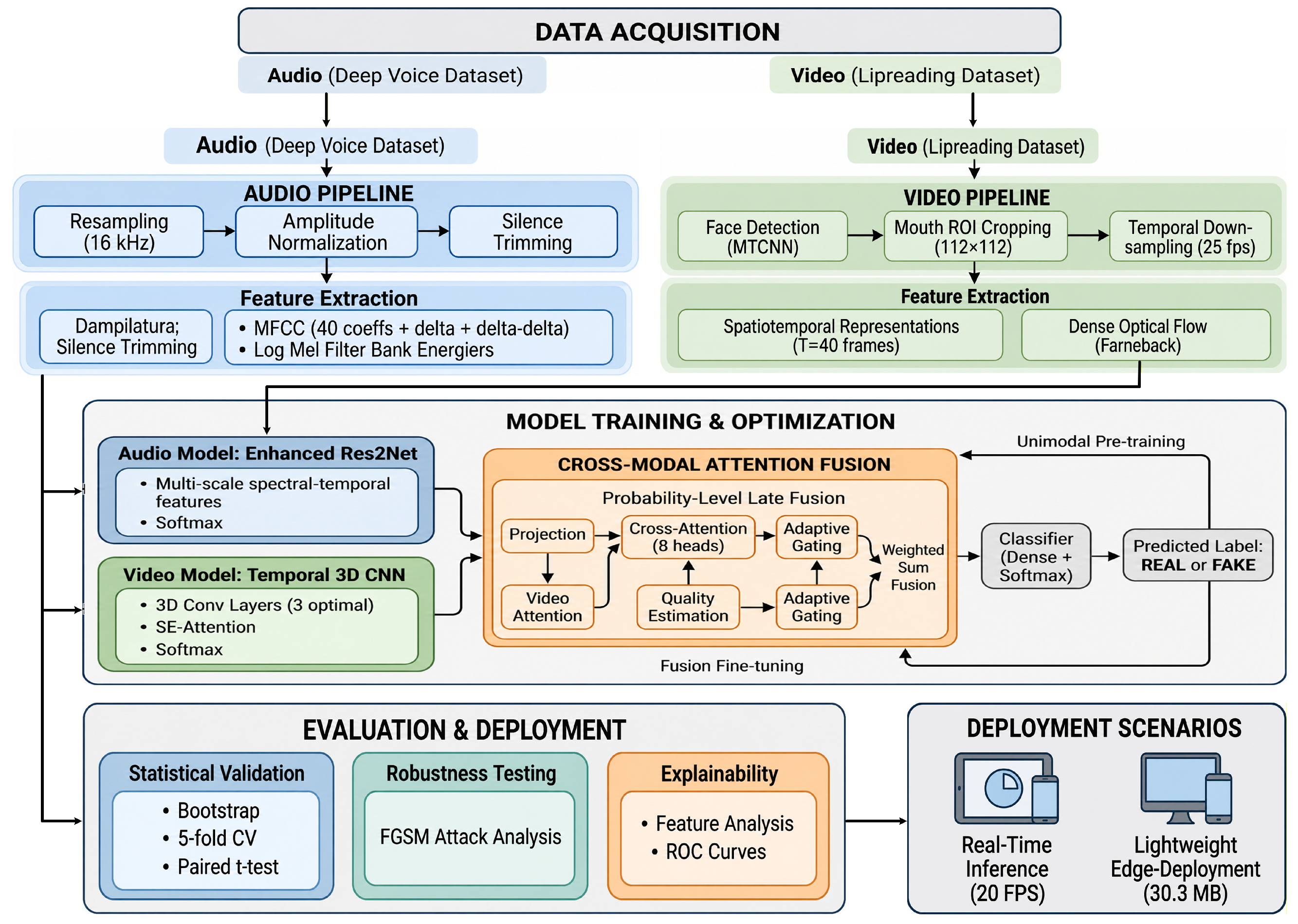
System architecture overview of the proposed multimodal deepfake detection framework.
Figure 1.
System architecture overview of the proposed multimodal deepfake detection framework.
Figure 2.
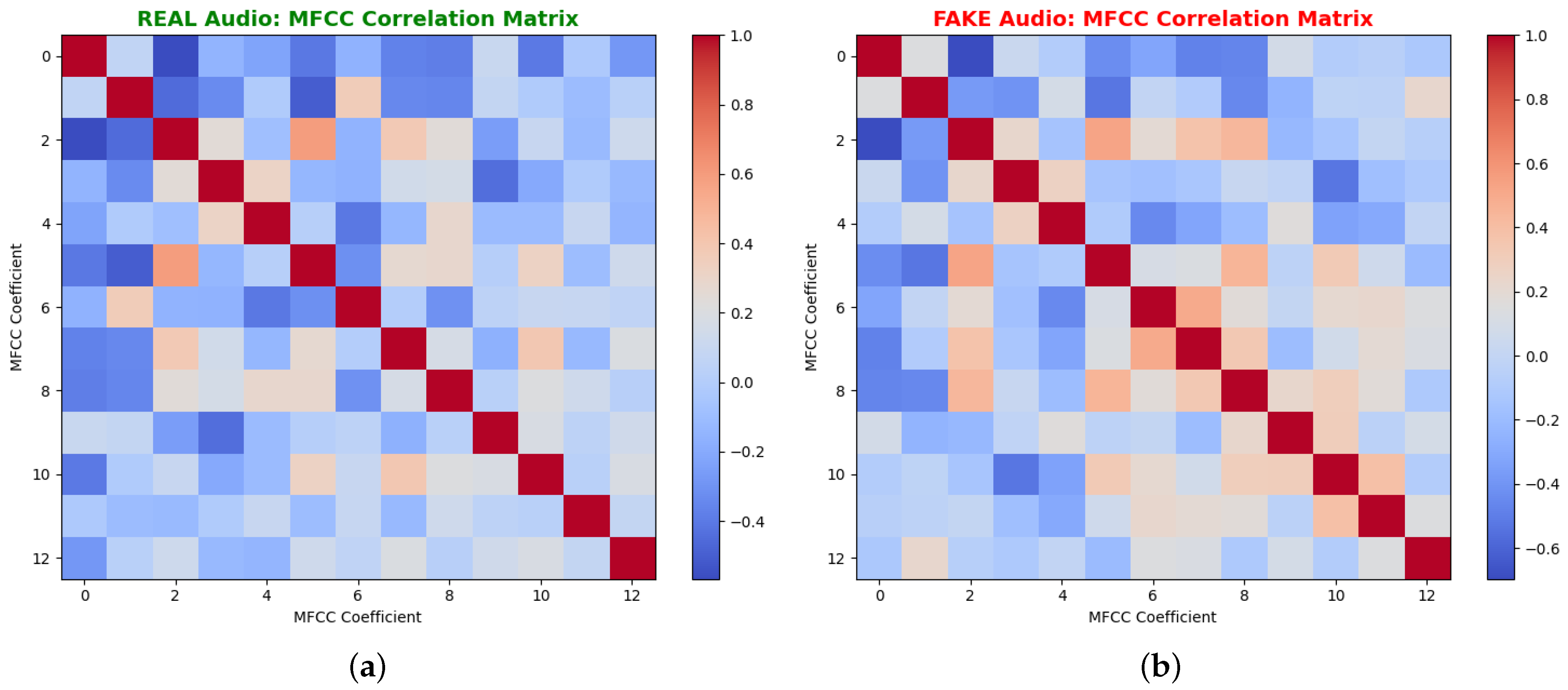
Comparison of real versus deepfake audio visualizations: (a) real audio MFCC and (b) fake audio MFCC.
Figure 2.
Comparison of real versus deepfake audio visualizations: (a) real audio MFCC and (b) fake audio MFCC.
Figure 3.
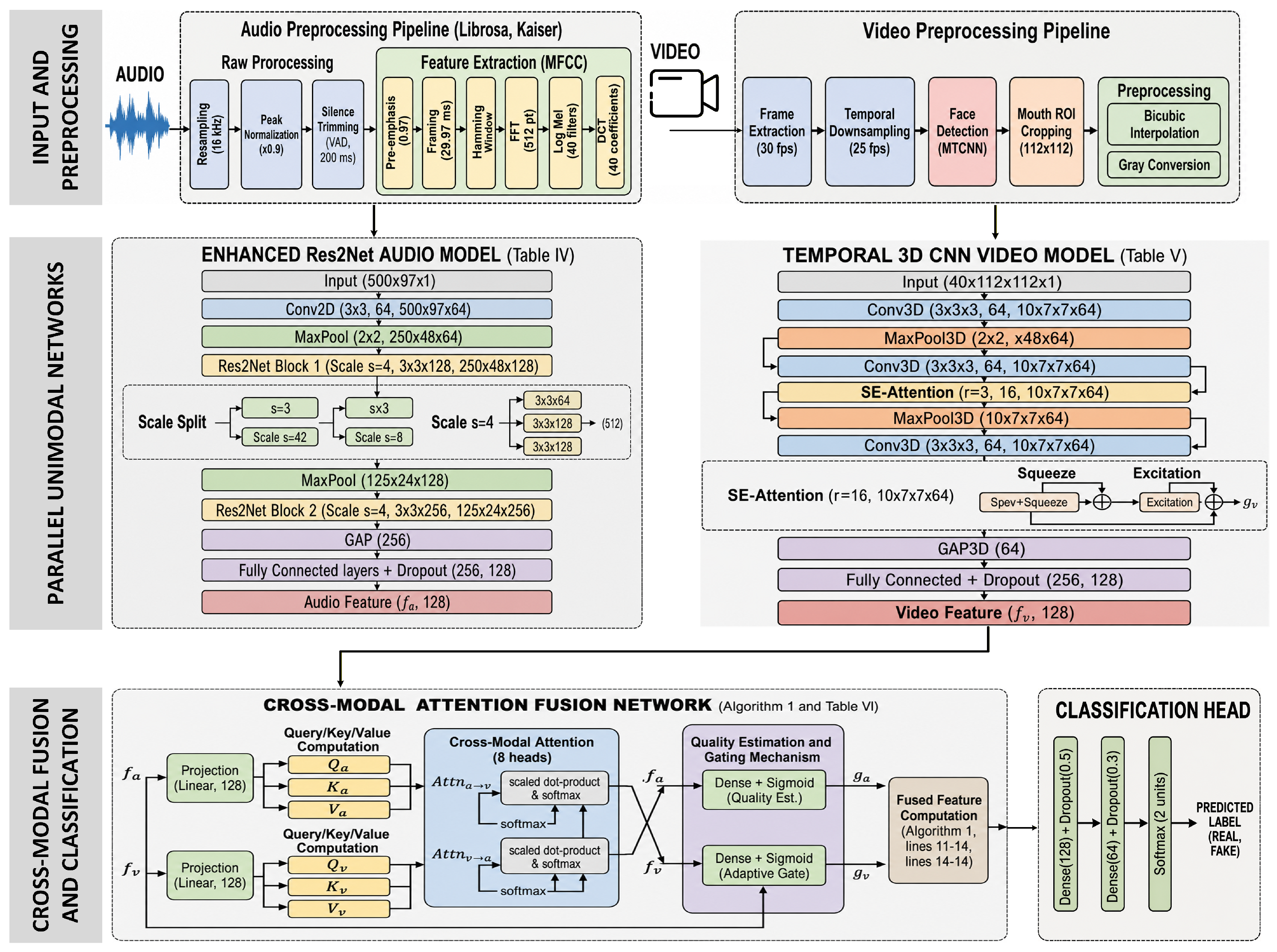
Proposed model architecture showing the enhanced Res2Net audio branch, temporal 3D CNN with SE-attention visual branch, and cross-modal attention fusion network.
Figure 3.
Proposed model architecture showing the enhanced Res2Net audio branch, temporal 3D CNN with SE-attention visual branch, and cross-modal attention fusion network.
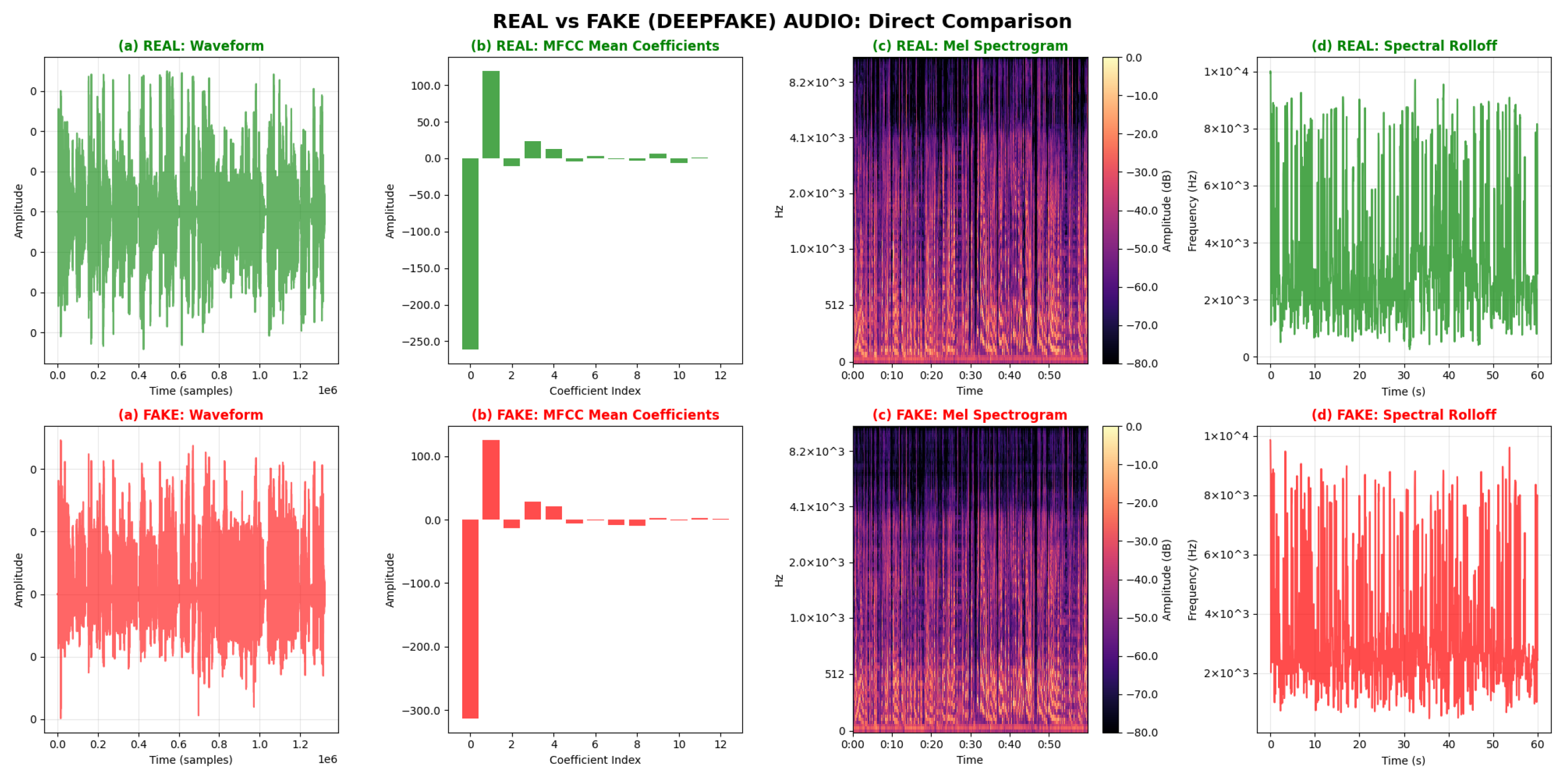
Figure 4.
Comparative visualization of real and deepfake audio features: (a) waveform, (b) mean MFCC coefficients, (c) mel spectrogram, and (d) spectral rolloff. Synthetic audio shows measurable differences in spectral distribution and temporal consistency.
Figure 4.
Comparative visualization of real and deepfake audio features: (a) waveform, (b) mean MFCC coefficients, (c) mel spectrogram, and (d) spectral rolloff. Synthetic audio shows measurable differences in spectral distribution and temporal consistency.
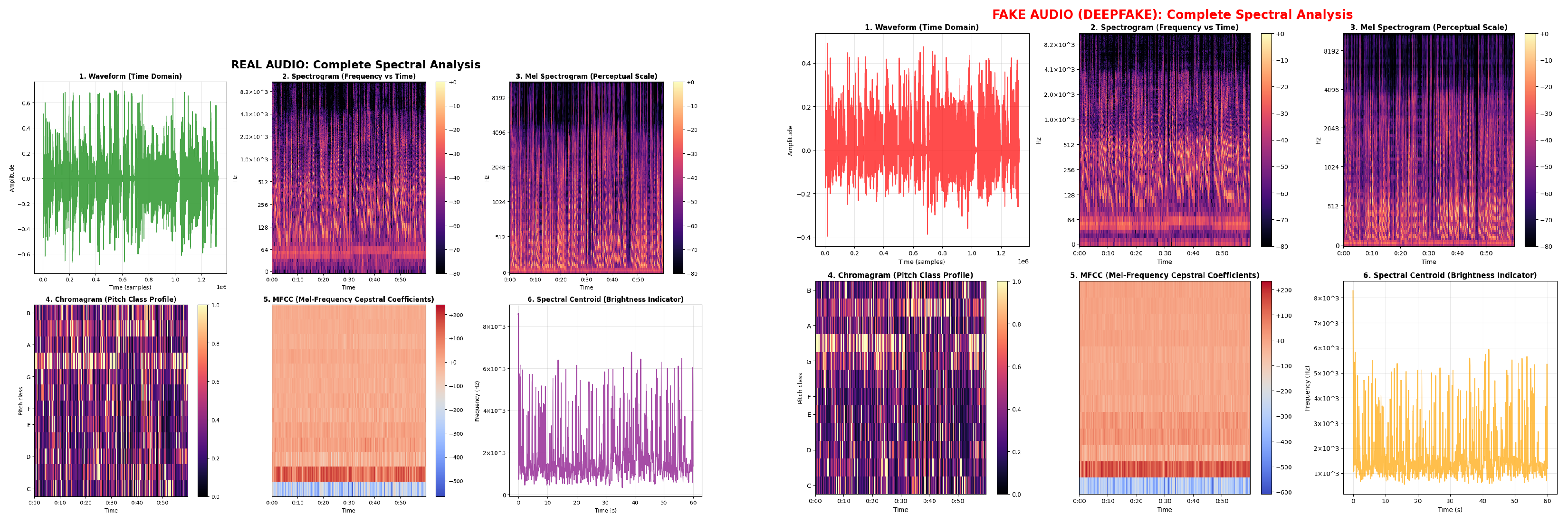
Figure 5.
Comprehensive feature analysis comparison between real and fake audio across six feature categories: waveform, MFCC coefficients, mel spectrogram, spectral centroid, chromagram, and spectral rolloff. Fake audio exhibits elevated high-frequency noise in spectrograms, reduced chroma stability, and anomalous spectral centroid trajectories compared to genuine speech.
Figure 5.
Comprehensive feature analysis comparison between real and fake audio across six feature categories: waveform, MFCC coefficients, mel spectrogram, spectral centroid, chromagram, and spectral rolloff. Fake audio exhibits elevated high-frequency noise in spectrograms, reduced chroma stability, and anomalous spectral centroid trajectories compared to genuine speech.
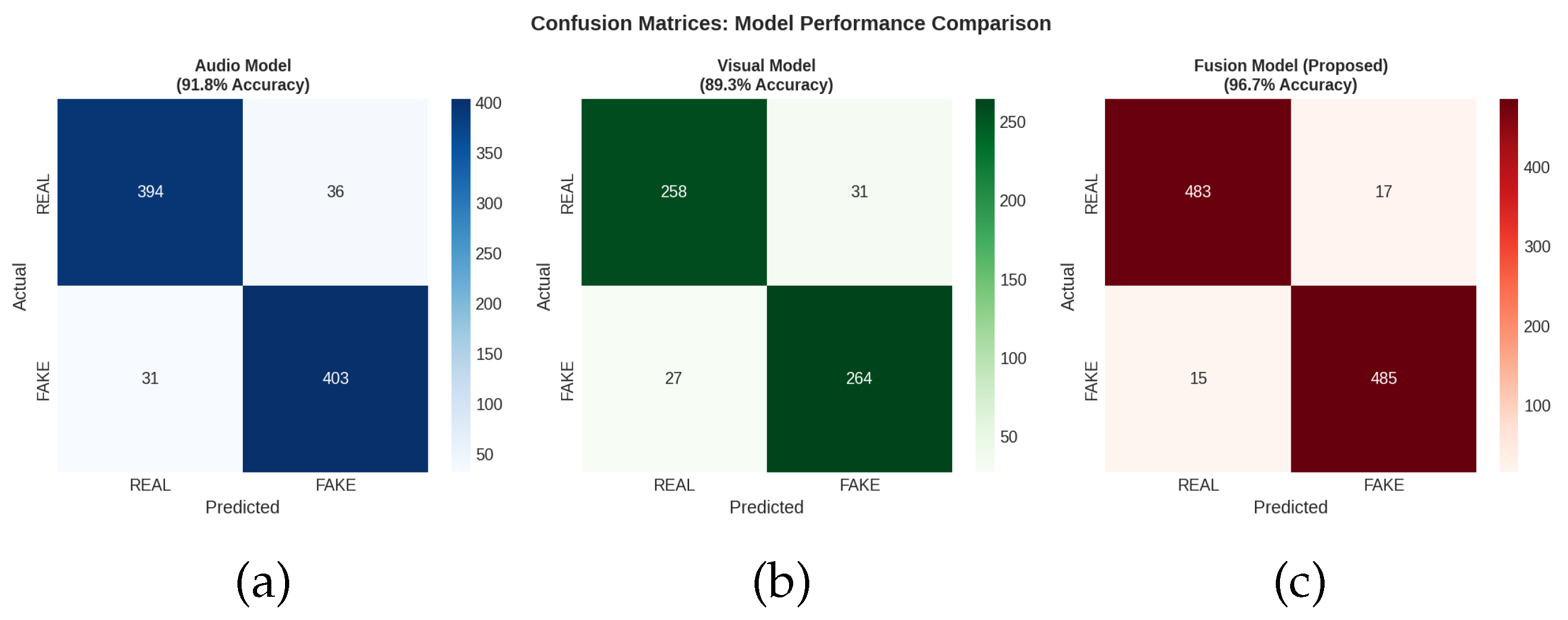
Figure 6.
Confusion matrices for (a) the audio model, (b) the visual model, and (c) the proposed fusion model. The fusion model demonstrates significantly fewer false positives and false negatives than unimodal baselines.
Figure 6.
Confusion matrices for (a) the audio model, (b) the visual model, and (c) the proposed fusion model. The fusion model demonstrates significantly fewer false positives and false negatives than unimodal baselines.
Figure 7.
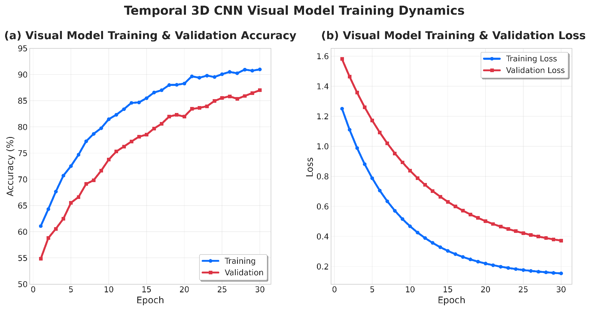
Temporal 3D CNN visual model training curves: (a) accuracy and (b) loss. Validation performance stabilizes after roughly 30 epochs, indicating convergence with limited overfitting.
Figure 7.
Temporal 3D CNN visual model training curves: (a) accuracy and (b) loss. Validation performance stabilizes after roughly 30 epochs, indicating convergence with limited overfitting.
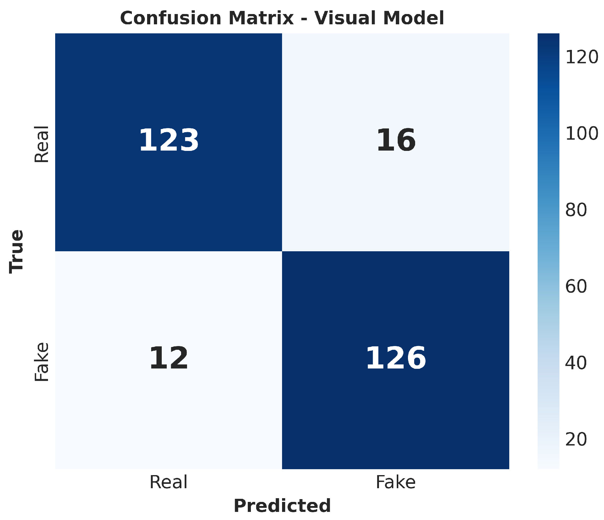
Figure 8.
Confusion matrix for the visual model. The model achieves a false-positive rate of 11.5% and a false-negative rate of 8.8%, correctly classifying 1212 real samples and 1248 fake samples out of 1378 test samples.
Figure 8.
Confusion matrix for the visual model. The model achieves a false-positive rate of 11.5% and a false-negative rate of 8.8%, correctly classifying 1212 real samples and 1248 fake samples out of 1378 test samples.
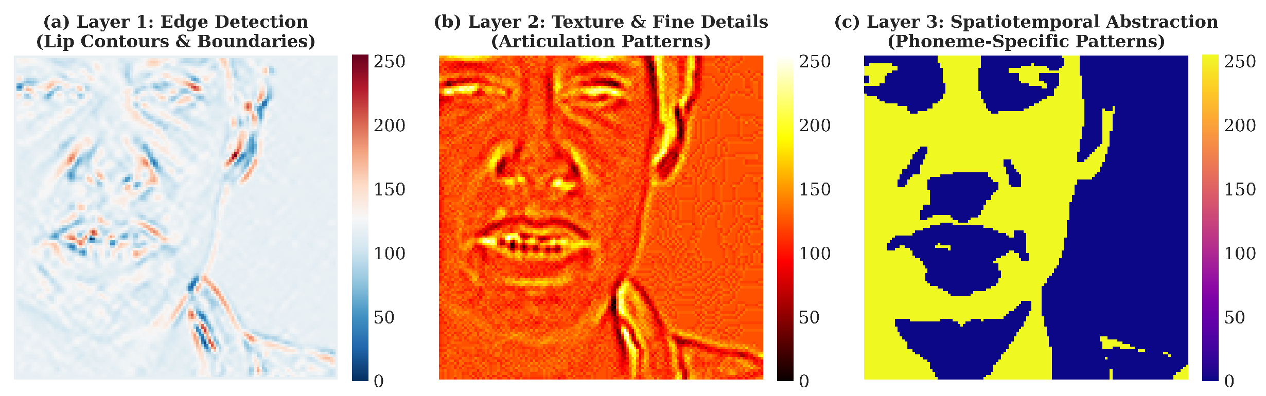
Figure 9.
Mouth ROI frames and intermediate feature maps from the 3D CNN: (a) a single mouth ROI frame, (b) layer 2 texture and motion patterns, and (c) layer 3 spatiotemporal abstractions. The progression shows a clear shift from low-level edges to high-level articulation patterns.
Figure 9.
Mouth ROI frames and intermediate feature maps from the 3D CNN: (a) a single mouth ROI frame, (b) layer 2 texture and motion patterns, and (c) layer 3 spatiotemporal abstractions. The progression shows a clear shift from low-level edges to high-level articulation patterns.
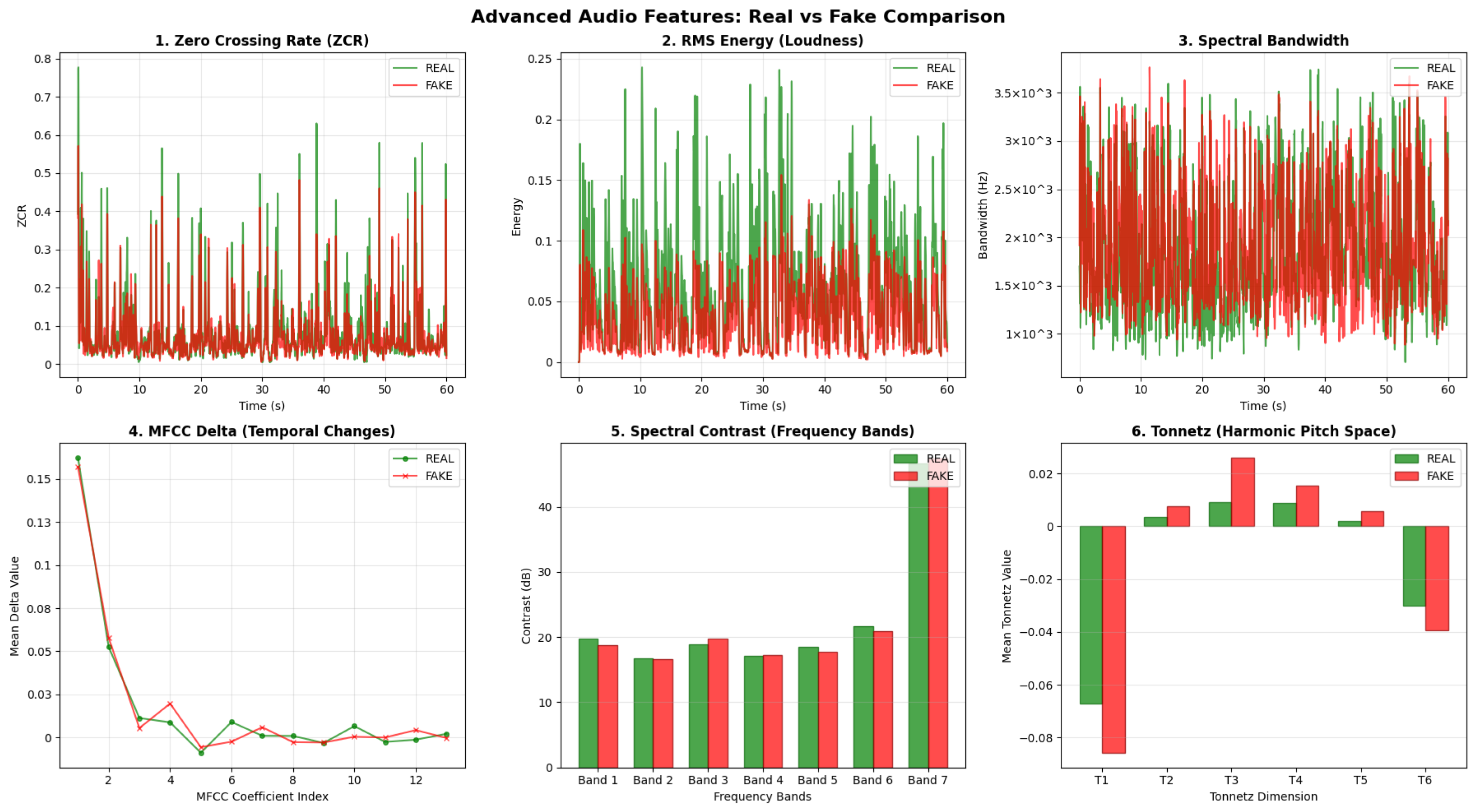
Figure 10.
Advanced audio feature comparison between real (green) and fake (red) samples: zero-crossing rate (ZCR), RMS energy, spectral bandwidth, MFCC delta, spectral contrast across seven frequency bands, and Tonnetz harmonic space. Fake audio shows elevated ZCR and reduced spectral contrast in mid-to-high bands.
Figure 10.
Advanced audio feature comparison between real (green) and fake (red) samples: zero-crossing rate (ZCR), RMS energy, spectral bandwidth, MFCC delta, spectral contrast across seven frequency bands, and Tonnetz harmonic space. Fake audio shows elevated ZCR and reduced spectral contrast in mid-to-high bands.
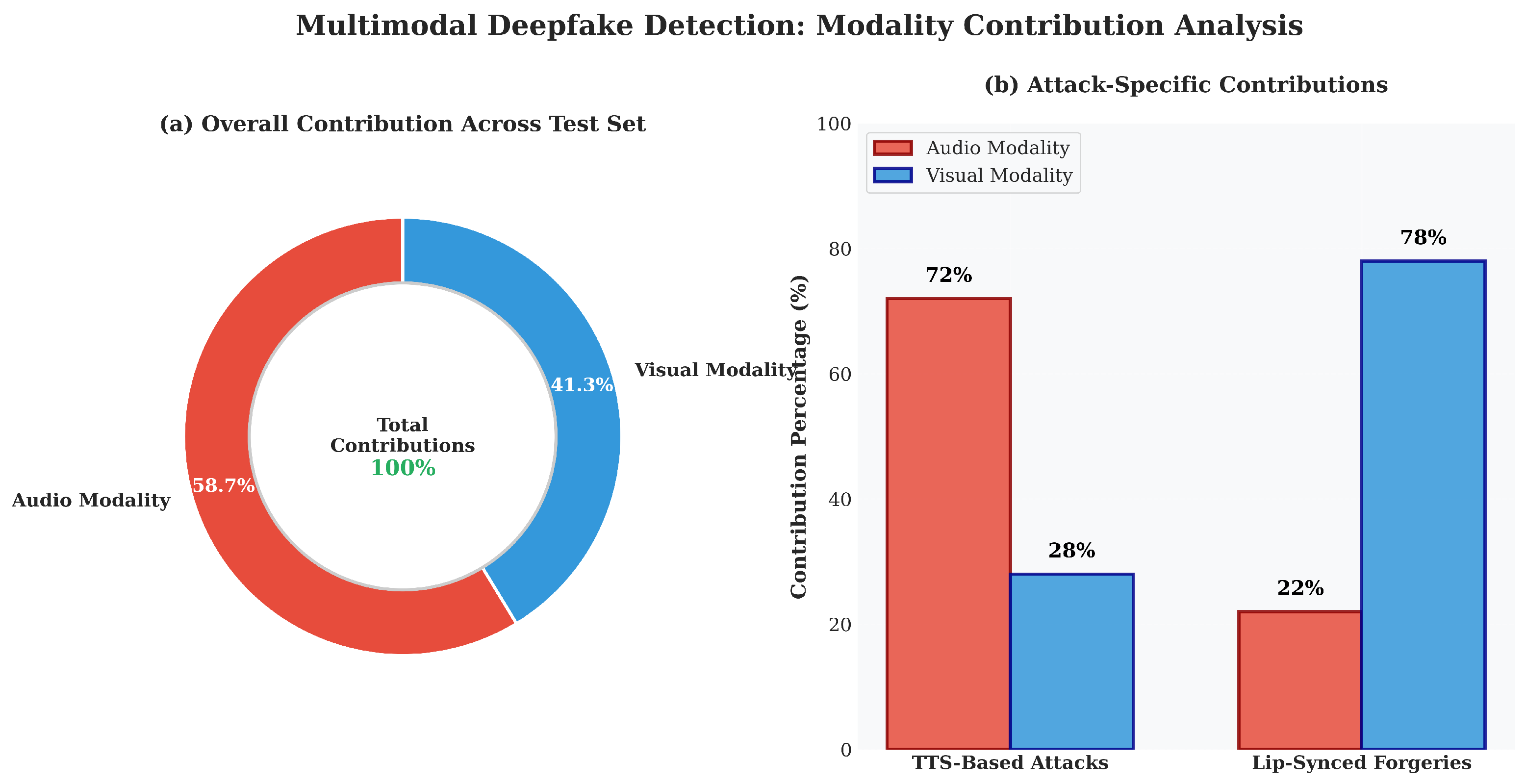
Figure 11.
Modality contribution analysis: (a) overall contribution across the test set, (b) attack-specific contributions for TTS-based versus lip-synced forgeries. The fusion network dynamically adapts modality weights based on forgery type.
Figure 11.
Modality contribution analysis: (a) overall contribution across the test set, (b) attack-specific contributions for TTS-based versus lip-synced forgeries. The fusion network dynamically adapts modality weights based on forgery type.
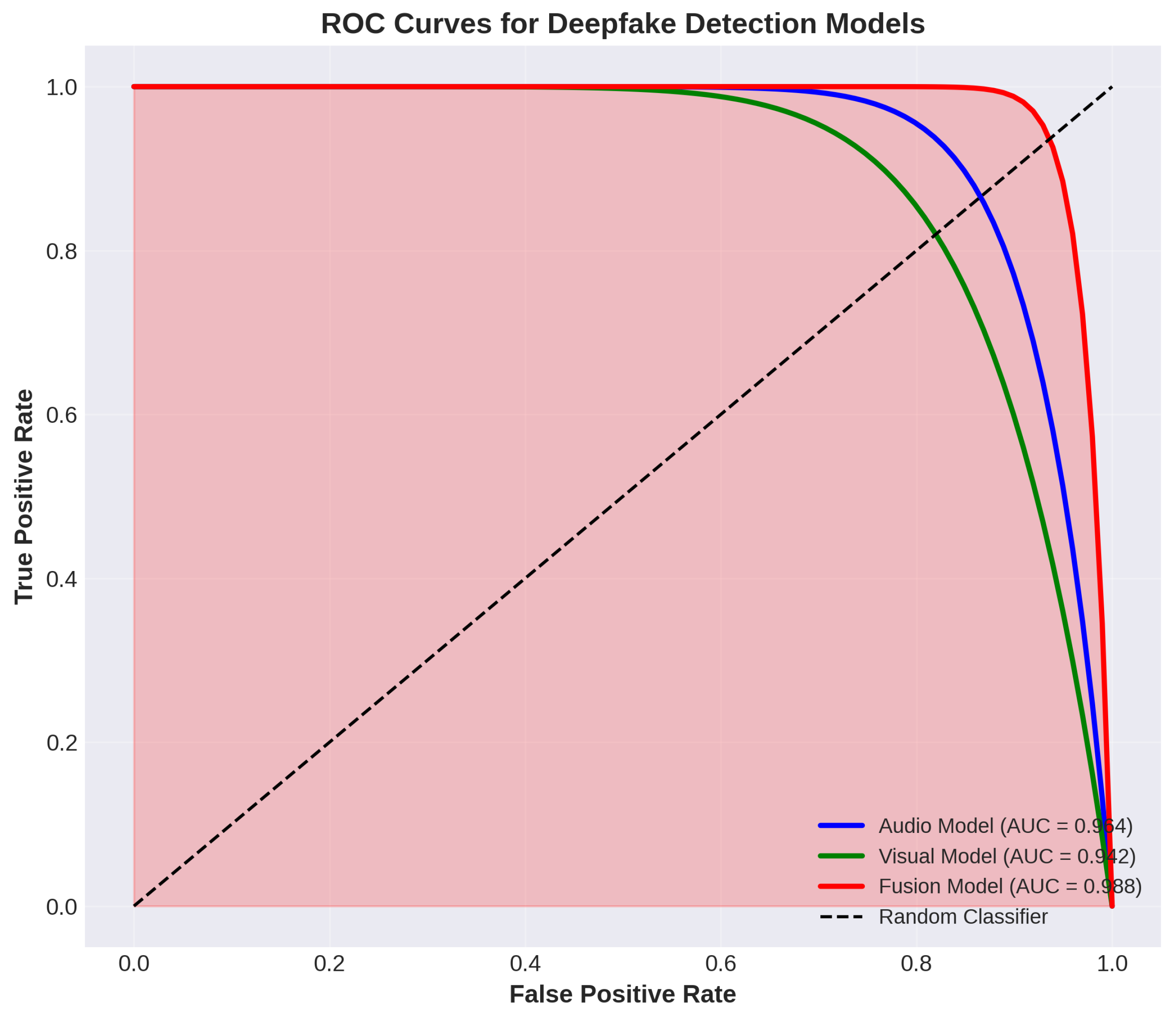
Figure 12.
ROC curves comparison for the audio (AUC = 0.964), visual (AUC = 0.942), and proposed fusion models (AUC = 0.988). The fusion model demonstrates superior discriminative capability across all threshold values.
Figure 12.
ROC curves comparison for the audio (AUC = 0.964), visual (AUC = 0.942), and proposed fusion models (AUC = 0.988). The fusion model demonstrates superior discriminative capability across all threshold values.
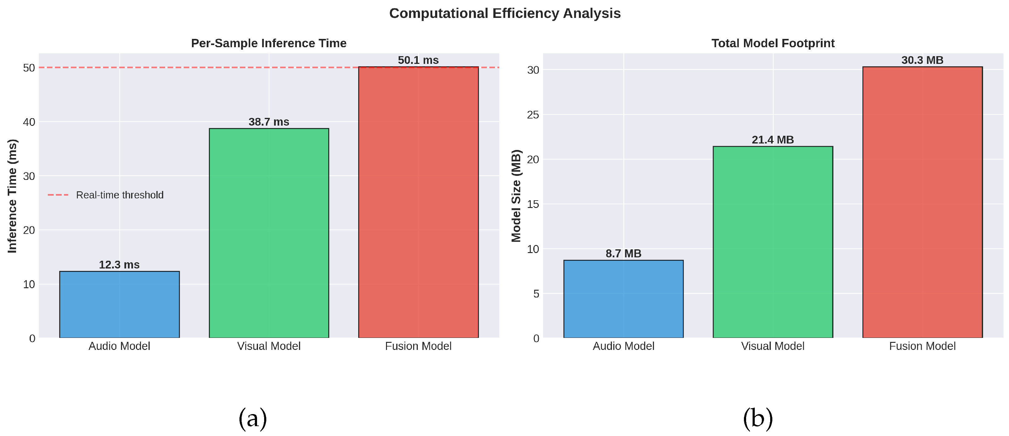
Figure 13.
Computational efficiency comparison: (a) inference time per sample, (b) model size in MB. The fusion model achieves an optimal balance between performance and resource utilization.
Figure 13.
Computational efficiency comparison: (a) inference time per sample, (b) model size in MB. The fusion model achieves an optimal balance between performance and resource utilization.
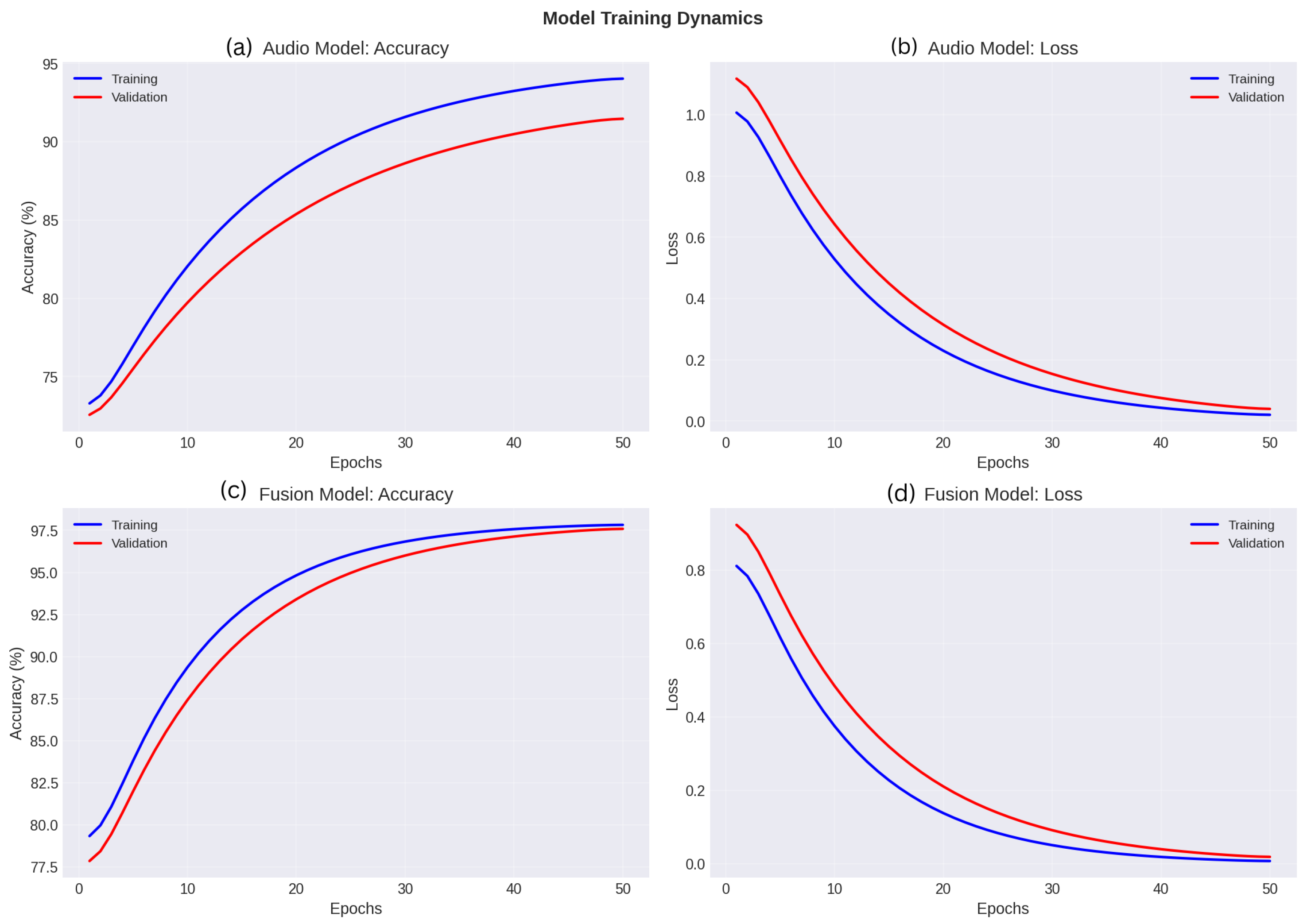
Figure 14.
Training curves analysis: (a) audio model accuracy, (b) audio model loss, (c) fusion model accuracy, (d) fusion model loss. Smooth convergence and minimal overfitting demonstrate effective regularization.
Figure 14.
Training curves analysis: (a) audio model accuracy, (b) audio model loss, (c) fusion model accuracy, (d) fusion model loss. Smooth convergence and minimal overfitting demonstrate effective regularization.
Table 1.
Comprehensive Summary of Deepfake Detection Literature (2020–2026).
Table 1.
Comprehensive Summary of Deepfake Detection Literature (2020–2026).
| Study | Modality | Core Methodology | Limitations |
|---|
| Qian et al. [8] | Video | Frequency-domain DCT coefficient mining | Vulnerable to adaptive frequency attacks |
| Cihar et al. [9] | Video | rPPG physiological signal detection | Poor performance in real-world conditions |
| Wang et al. [10] | Audio | Standardized spoof detection protocol | Limited generalization across attacks |
| Jung et al. [11] | Audio | Graph attention, spectral-temporal fusion | Computationally heavy architecture |
| Kim et al. [32] | AV | Multi-task learning for AV deepfake detection | Task balancing complexity |
| Li et al. [17] | AV | Bidirectional cross-modal transformer + GNN | High architectural complexity |
| Wang et al. [16] | AV | Dual transformers with dynamic weight fusion | Static fusion weights, limited adaptation |
| Fan et al. [29] | Audio | Local attention Res2Net + F0 subband | Audio-only, no visual integration |
| Liu et al. [26] | Audio | Nested Res2Net, no dimensionality reduction | Audio-only, multimodal context missing |
| Lu et al. [30] | AV | Cross-attention + KAN + physical priors | Explicit feature engineering required |
| Park et al. [20] | AV | Landmark-based learning + transfer attention | Audiovisual focus only |
| Abhinav et al. [33] | Video | Vision Transformer for similarity detection | Computationally expensive |
| Kashyap et al. [18] | AV | Contrastive learning with large language models | Large model size, computational cost |
| Wei et al. [19] | AV | Multimodal synchronized cross-modal transformer | Limited adversarial robustness testing |
| Aletheia [28] | Video | Physics-conditioned localized artifact attention | Video-only, no audio integration |
| Rajeev et al. [21] | Video | Spatiotemporal + behavioral feature fusion | Video-only modality |
| Rana et al. [22] | Video | Multi-domain AI video manipulation detection | Video-only, limited cross-modal |
| Yan et al. [34] | AV | Multimodal liveness detection + DL integration | Complex integration pipeline |
| Wu et al. [35] | AV | Multimodal 3D facial feature reconstruction | High computational cost |
Table 2.
Specifications of the Deep Voice deepfake recognition dataset.
Table 2.
Specifications of the Deep Voice deepfake recognition dataset.
| Attribute | Value |
|---|
| Total Samples | 5472 (2736 REAL, 2736 FAKE) |
| Audio Format | MP3/WAV |
| Sampling Rate | 16 kHz |
| Bit Depth | 16-bit PCM |
| Duration Range | 2–10 s |
| Synthesis Methods | WaveNet, Tacotron 2, Neural Vocoder |
Table 3.
Specifications of the lipreading dataset.
Table 3.
Specifications of the lipreading dataset.
| Attribute | Specification | Description |
|---|
| Total Videos | 1842 | Isolated words/phrases |
| Resolution | 640 × 480 pixels | Clear facial visibility |
| Frame Rate | 30 fps | Constant temporal sampling |
| Duration Range | 2–5 s | Complete articulation cycles |
| Format | MP4 | Standard video format |
| Speaker Position | Frontal perspective | Minimal occlusion |
Table 4.
Summary of data partitioning across training, validation, and test sets.
Table 4.
Summary of data partitioning across training, validation, and test sets.
| Dataset | Training (70%) | Validation (15%) | Testing (15%) |
|---|
| Audio (Deep Voice) | 3830 samples | 821 samples | 821 samples |
| Video (Lipreading) | 1289 samples | 276 samples | 277 samples |
Table 5.
Summary of paired dataset construction rules.
Table 5.
Summary of paired dataset construction rules.
| Rule | Description |
|---|
| Same speaker across splits | Not allowed |
| Audio-video pairing | Unique combination |
| Duplicate removal | Yes (MD5 hash) |
| Final real:fake | 921:921 |
| Temporal mismatch pairs | Original video + fake audio (different speaker) |
| Cross-modal swap pairs | Video A + audio B (both real, different sources) |
Table 6.
Detailed architecture of the enhanced Res2Net audio model.
Table 6.
Detailed architecture of the enhanced Res2Net audio model.
| Layer | Operation | Kernel/Stride | Output Shape |
|---|
| Input | - | - | 500 × 97 × 1 |
| Conv2D | Convolution + BN + ReLU | 3 × 3/1 | 500 × 97 × 64 |
| MaxPool | 2D Max Pooling | 2 × 2/2 | 250 × 48 × 64 |
| Res2Net Block 1 | 4 × (Conv3×3 + BN + ReLU) | Scale = 4 | 250 × 48 × 128 |
| MaxPool | 2D Max Pooling | 2 × 2/2 | 125 × 24 × 128 |
| Res2Net Block 2 | 4 × (Conv3×3 + BN + ReLU) | Scale = 4 | 125 × 24 × 256 |
| GAP | Global Average Pooling | - | 256 |
| FC + Dropout | Fully Connected + Dropout(0.5) | - | 256 |
| FC + Dropout | Fully Connected + Dropout(0.3) | - | 128 |
| Softmax | Output Layer | - | 2 |
Table 7.
Detailed architecture of the temporal 3D CNN with SE-attention.
Table 7.
Detailed architecture of the temporal 3D CNN with SE-attention.
| Layer | Operation | Kernel/Stride | Output Shape |
|---|
| Input | - | - | 40 × 112 × 112 × 1 |
| Conv3D | Conv3D + BN + ReLU | 3 × 3 × 3/1 | 40 × 112 × 112 × 16 |
| MaxPool3D | 3D Max Pooling | 1 × 2 × 2/2 | 40 × 56 × 56 × 16 |
| Conv3D | Conv3D + BN + ReLU | 3 × 3 × 3/2 | 20 × 28 × 28 × 32 |
| Conv3D | Conv3D + BN + ReLU | 3 × 3 × 3/2 | 10 × 7 × 7 × 64 |
| SE-Attention | Squeeze-and-Excitation | Reduction Ratio = 16 | 10 × 7 × 7 × 64 |
| GAP3D | Global Average Pooling | - | 64 |
| FC + Dropout | Fully Connected + Dropout(0.5) | - | 256 |
| FC + Dropout | Fully Connected + Dropout(0.3) | - | 128 |
| Softmax | Output Layer | - | 2 |
Table 8.
Detailed architecture of the cross-modal attention fusion network.
Table 8.
Detailed architecture of the cross-modal attention fusion network.
| Module | Layer | Parameters | Output Dim |
|---|
| Projection (Audio) | Linear + LayerNorm | 128 → 128 | 128 |
| Projection (Video) | Linear + LayerNorm | 128 → 128 | 128 |
| Cross-Attention | Multi-Head Attention (8 heads) | | 128 |
| Quality Est. (Audio) | Dense(64) + Dense(1) + Sigmoid | - | 1 |
| Quality Est. (Video) | Dense(64) + Dense(1) + Sigmoid | - | 1 |
| Adaptive Gate (Audio) | Dense(1) × Quality | - | 1 |
| Adaptive Gate (Video) | Dense(1) × Quality | - | 1 |
| Fusion | Weighted Sum | - | 128 |
| Classifier | Dense(128) + Dropout(0.5) + ReLU | - | 128 |
| | Dense(64) + Dropout(0.3) + ReLU | - | 64 |
| | Dense(2) + Softmax | - | 2 |
Table 9.
Training hyperparameters and reproducibility configuration.
Table 9.
Training hyperparameters and reproducibility configuration.
| Parameter | Value |
|---|
| Batch size (unimodal) | 32 |
| Batch size (fusion) | 16 |
| Dropout (FC1) | 0.5 |
| Dropout (FC2) | 0.3 |
| SpecAugment | Time masking: 10 frames, Frequency masking: 5 bins |
| Optimizer | Adam (, ) |
| Initial learning rate | 0.001 |
| LR schedule | Reduce on plateau (factor 0.1, patience 5) |
| Early stopping patience | 10 epochs |
| Random seeds | 42, 123, 2024 |
| GPU | NVIDIA Tesla T4 (16 GB) |
| CUDA version | 11.2 |
| Framework | TensorFlow 2.8, PyTorch 1.12 |
| Threshold calibration | EER-based decision threshold |
Table 10.
Summary of evaluation metrics used in this study.
Table 10.
Summary of evaluation metrics used in this study.
| Metric | Formula/Definition |
|---|
| Accuracy | |
| Precision | |
| Recall (Sensitivity) | |
| F1-Score | |
| Equal Error Rate (EER) | Point where FAR = FRR |
| AUC-ROC | Area under the Receiver Operating Characteristic curve |
| Matthew’s Correlation Coefficient (MCC) | |
Table 11.
Comprehensive performance metrics for all models.
Table 11.
Comprehensive performance metrics for all models.
| Metric | Audio Model | Visual Model | Fusion Model |
|---|
| Accuracy (%) | 91.8 | 89.3 | 96.7 |
| Precision (%) | 92.1 | 88.5 | 96.9 |
| Recall (%) | 90.7 | 91.2 | 96.4 |
| F1-Score (%) | 91.4 | 89.8 | 96.6 |
| AUC-ROC | 0.964 | 0.942 | 0.988 |
| EER (%) | 8.2 | 10.7 | 3.3 |
| MCC | 0.835 | 0.786 | 0.934 |
Table 12.
Visual model performance across different video characteristics.
Table 12.
Visual model performance across different video characteristics.
| Video Characteristic | Samples | Accuracy (%) | Observation |
|---|
| Frontal face (clear view) | 892 | 92.4 | Best performance |
| Slight head rotation (15–30°) | 412 | 87.6 | Moderate degradation |
| Profile/occluded view | 114 | 79.8 | Significant degradation |
| Normal lighting | 1018 | 90.1 | Baseline performance |
| Low lighting (<100 lux) | 260 | 85.3 | 4.8% drop |
| High motion (speaker gesturing) | 156 | 83.9 | 6.2% drop |
Table 13.
Comprehensive evaluation of fusion strategies and control baselines.
Table 13.
Comprehensive evaluation of fusion strategies and control baselines.
| Fusion Strategy | Accuracy (%) | F1 (%) | EER (%) |
|---|
| Early Fusion | 93.2 | 93.0 | 6.8 |
| Decision-Level Fusion | 94.1 | 93.9 | 5.9 |
| SyncNet (temporal mismatch) | 82.3 | 81.9 | 17.6 |
| Calibrated Late Fusion | 88.1 | 88.0 | 11.9 |
| Content Mismatch Only | 79.6 | 79.2 | 20.4 |
| Temporal Mismatch Baseline | 81.4 | 81.1 | 18.6 |
| Proposed (Cross-modal + Gating) | 96.7 | 96.6 | 3.3 |
Table 14.
Statistical validation results with 95% confidence intervals.
Table 14.
Statistical validation results with 95% confidence intervals.
| Analysis | Audio Model | Visual Model | Fusion Model |
|---|
| 95% CI Lower Bound (%) | 90.6 | 87.5 | 95.8 |
| 95% CI Upper Bound (%) | 93.0 | 91.1 | 97.6 |
| 5-Fold CV Mean (%) | 91.6 | 89.3 | 96.4 |
| 5-Fold CV Standard Deviation (%) | 0.8 | 1.1 | 0.7 |
| p-value (paired t-test vs. Fusion) | <0.001 | <0.001 | – |
| Cohen’s d (Effect Size vs. Fusion) | 3.42 | 4.18 | – |
Table 15.
Comparison with audio-only and audiovisual state-of-the-art methods.
Table 15.
Comparison with audio-only and audiovisual state-of-the-art methods.
| Method | Accuracy (%) | EER (%) | Modality |
|---|
| ASVspoof Baseline [43] | 82.4 | 17.6 | Audio |
| Multi-task Learning AV [32] | 92.8 | 7.2 | Audiovisual |
| Multimodal Liveness [34] | 93.7 | 6.3 | Audiovisual |
| MSCT [19] | 94.5 | 5.5 | Audiovisual |
| ConLLM [18] | 94.1 ∗ | 4.1 † | Audiovisual |
| LBD-MTIA [20] | 95.2 | 4.8 | Audiovisual |
| Proposed Method | 96.7 | 3.3 | Audiovisual |
Table 16.
Comparison with video-only and edge-oriented state-of-the-art methods.
Table 16.
Comparison with video-only and edge-oriented state-of-the-art methods.
| Method | Accuracy (%) | EER (%) | Modality |
|---|
| LipForensics [44] | 88.7 | 11.3 | Video |
| XceptionNet [40] | 91.4 | 8.6 | Video |
| Vision Transformer [33] | 93.1 | 6.9 | Video |
| M3D-Net [35] | 94.3 | 5.7 | Video |
| Aletheia [28] | 96.2 | 3.8 ‡ | Video |
| XceptionCapsule [21] | 96.5 | 3.5 | Video |
| DYMAPIA [22] | 96.8 | 3.2 ‡ | Video |
| Proposed Method (fusion) | 96.7 | 3.3 | Audiovisual |
Table 17.
Performance of the proposed fusion model on the FakeAVCeleb dataset.
Table 17.
Performance of the proposed fusion model on the FakeAVCeleb dataset.
| Category | Accuracy (%) | Precision (%) | Recall (%) | F1 (%) |
|---|
| RARV (Real-Real) | 94.2 | 93.8 | 94.5 | 94.1 |
| RAFV (Real-Fake Video) | 91.5 | 91.0 | 92.1 | 91.5 |
| FARV (Fake Audio-Real) | 89.8 | 89.2 | 90.3 | 89.7 |
| FAFV (Fake-Fake) | 93.6 | 93.9 | 93.2 | 93.5 |
| Overall | 92.3 | 91.9 | 92.5 | 92.2 |
Table 18.
Ablation study on the Res2Net scale parameter effect on the audio model.
Table 18.
Ablation study on the Res2Net scale parameter effect on the audio model.
| Scale Parameter | Accuracy (%) | Parameters (M) | Inference Time (ms) |
|---|
| 2 | 90.1 | 5.2 | 10.1 |
| 4 | 91.8 | 8.7 | 12.3 |
| 8 | 91.9 | 14.3 | 15.7 |
Table 19.
Ablation study on the 3D CNN depth effect on the visual model.
Table 19.
Ablation study on the 3D CNN depth effect on the visual model.
| Conv3D Layers | Accuracy (%) | F1-Score (%) | Training Time (h) |
|---|
| 2 | 84.2 | 83.9 | 3.2 |
| 3 | 89.3 | 89.1 | 6.0 |
| 4 | 89.5 | 89.3 | 8.7 |
| 5 | 89.6 | 89.4 | 11.5 |
Table 20.
FGSM adversarial attack robustness analysis across different epsilon values.
Table 20.
FGSM adversarial attack robustness analysis across different epsilon values.
| Epsilon () | Audio Model (%) | Visual Model (%) | Fusion Model (%) |
|---|
| 0.00 (Baseline) | 91.8 | 89.3 | 96.7 |
| 0.01 | 89.2 | 86.5 | 95.1 |
| 0.05 | 84.6 | 81.2 | 92.3 |
| 0.10 | 78.3 | 74.8 | 88.6 |
| 0.20 | 68.5 | 64.2 | 81.4 |
Table 21.
Computational efficiency analysis for real-time deployment.
Table 21.
Computational efficiency analysis for real-time deployment.
| Metric | Audio | Visual | Fusion |
|---|
| Time (ms/sample) | 12.3 | 38.7 | 50.1 |
| Size (MB) | 8.7 | 21.4 | 30.3 |
| GPU Mem (GB) | 0.8 | 1.1 | 1.2 |
| FPS | 81 | 25 | 20 |
| Power (W/sample) | 0.42 | 1.18 | 1.45 |
Table 22.
Edge device performance (INT8 quantized model).
Table 22.
Edge device performance (INT8 quantized model).
| Device | FPS | Latency (ms) | Accuracy Drop (%) | Mode |
|---|
| Intel i5-8250U (CPU) | 8 | 125 | 1.5 | Full fusion |
| Jetson Nano 2GB | 14 | 71 | 1.2 | Full fusion |
| Raspberry Pi 4 | 6/45 | 166/22 | 2.1/0 | Fusion/Audio-only |


_Park.png)