Appendix A. Proof of Theorem 1
Traditional shallow convolutional neural networks with convolution kernels exhibit inherent proficiency in extracting small objects and non-edge features.
Proof. Consider a CNN
with input tensor
. The first convolutional layer
employs
kernels
with stride 1 and padding 1, generating feature maps:
where
denotes the activation function. □
Part 1: Small Object Extraction Capability.
Define a small object with spatial diameter pixels (i.e., ). Let denote the receptive field centered at .
Lemma A1. For any satisfying , there exist coordinates such that .
Proof. By definition, is contained within a pixel region. Selecting as the centroid of the minimal axis-aligned bounding box containing satisfies the inclusion condition, with boundary handling guaranteed by the padding configuration. □
The activation strength for object
under kernel
d is quantified as
During gradient-based optimization,
the compact parameterization
induces a spatial inductive bias. The limited receptive field constrains kernels to specialize in local patterns within their
support, naturally prioritizing small object detection.
Part 2: Non-edge Feature Extraction Capability. Define a non-edge feature
as a local pattern satisfying
where
is an edge detection threshold.
Lemma A2. For any with , is fully contained within some receptive field .
Proof. Spatial constraints ensure resides within a region. Selecting as the center of this region guarantees under padding = 1. □
The representational capacity for
under kernel
d is quantified as
During optimization,
the compact parameterization induces a structural prior.
Lemma A3. For any edge feature with curvature , there exist distinct positions satisfying Proof. Curvature causes significant geometric divergence of edge segments within windows due to the discrete grid sampling. □
The constrained receptive field compels kernels to specialize in local pattern matching rather than global edge detection. By Lemma A3, edge features exhibit representation ambiguity while non-edge features satisfy
with minimal interference from edge components. Gradient descent therefore preferentially learns non-edge features within the
subspace.
Appendix B. Typical Flight Formation Configuration and Parameters
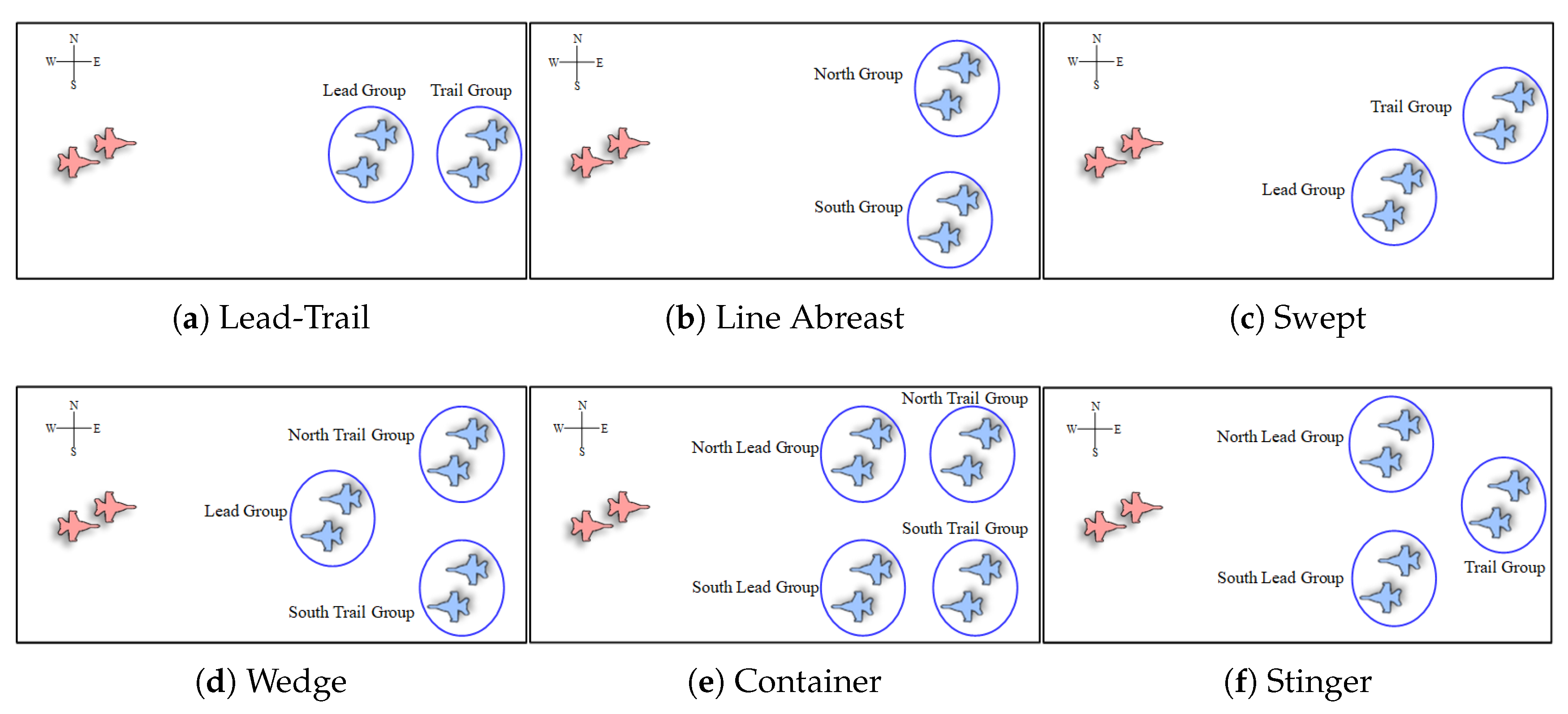
Flight groups often adopt specific formation configurations to enhance reconnaissance and combat capabilities. These formations typically fall into six main types: Lead-Trail, Line Abreast, Swept, Wedge, Container, and Stinger, categorized based on the positional arrangement of wingmen in the formation, as illustrated in
Figure A1.
Figure A1.
Typical flight formation.
Figure A1.
Typical flight formation.
The Lead-Trail formation typically comprises two to four aircraft, enabling efficient monitoring of wingmen and aerial situations to provide robust defensive support. The Line Abreast formation, consisting of two to four aircraft, offers extensive coverage of the attack zone, simplifying fire lane clearance and enabling effective attacks. Swept formations, also comprising two to four aircraft, provide flexibility for swift conversion into Lead-Trail or Line Abreast formations, making them ideal for low-altitude and adverse weather conditions. The Wedge formation, composed of three aircraft, facilitates tactical defense strategies, reduces the probability of hostile radar detection, and enables tactical deception. The Container formation, involving four aircraft, is commonly used for maintaining formation during cruising and executing specific air combat tactics such as the millstone. Lastly, the Stinger formation, comprising three aircraft, provides a clear forward BVR-fire channel and allows seamless support from the rear aircraft when needed.
The size and shape of formation configurations are adaptable and can be adjusted based on tactical considerations. Key parameters influencing the formation’s shape and size include depth, width, echelon, and slant in V-shape formations.
Figure A2 illustrates the crucial parameters in the formation, while
Table A1 details the specific value ranges of these key parameters as discussed in this paper.
Table A1.
Hyperparameter setting of flight formation.
Table A1.
Hyperparameter setting of flight formation.
| Parameters | Range |
|---|
| Aircraft spacing (km) | |
| Oblique range of Swept (rad) | |
| Angel range of Wedge/Stinger (rad) | |
| Horizontal and vertical noise (km) | |
| Course noise (rad) | |
| Formation numbers in one radar map | |
Figure A2.
Key parameters of the Stinger formation.
Figure A2.
Key parameters of the Stinger formation.
Appendix C. Visualization of the Feature Extraction Layers
ResNet18, ResNet50, and ResNet101 [
32] exhibit identical output image dimensions in their intermediate modules, with the primary difference being the number of convolutional layers across different modules. Theoretically, ResNet101 should at least match ResNet18 through an identity transformation, implying that ResNet101’s feature extraction capacity should exceed that of ResNet18. However, due to the uncontrollable nature of the network training, the actual feature extraction performance can vary between networks.
To investigate this, we applied the proposed image reconstruction method in a clustered scenario and passed the resulting images through the feature extraction networks to visualize key features within the network. Given the high number of image channels in the intermediate layers, we overlaid grayscale maps of each channel. The visualization results are presented in
Figure A3.
Figure A3.
Visualization of the feature extraction layers (ImageNet pretrained). The red boxes highlight the significant image features extracted by different feature extraction networks.
Figure A3.
Visualization of the feature extraction layers (ImageNet pretrained). The red boxes highlight the significant image features extracted by different feature extraction networks.
We tested the impact of varying formation numbers in an image and observed consistent trends. As the image size was compressed from 256 × 256 to 28 × 28, the performance of the three networks remained similar, with larger networks like ResNet101 yielding slightly clearer compressed features. However, as compression continued to 14 × 14 and 7 × 7, particularly with more than five formations in the image, the results became increasingly difficult to interpret. Notably, in the 7 × 7 features of the final layer, deeper networks often generated compressed features with fewer pixels than the number of formations, which could explain the loss of certain features in sparse images. While shallow networks exhibit coarser feature granularity, they maintain consistency in the overall feature count.
Appendix D. Pretraining Details
The first phase involves pre-training the E2I upsampling network using an autoencoder, as described in
Section 3.3. Training occurs over 50 epochs, with 200 iterations per epoch and a batch size of 256. We set the initial learning rate to 0.001, with a decay rate of 0.1 every 10 epochs. SmoothL1Loss is employed alongside the Adam optimizer.
Figure A4 showcases the convergence outcomes of the loss function during this training phase.
Figure A4.
The pre-training process for E2I-5. Different colors are employed to denote distinct learning rates.
Figure A4.
The pre-training process for E2I-5. Different colors are employed to denote distinct learning rates.
In the second step, a ResNet18 feature extraction network is trained using a supervised classification approach, freezing the pre-trained E2I upsampling network. This procedure aligns with the E2I-5 experiment in
Section 4.2.2 and is not reiterated here. We use PCA [
38] to visualize the compressed image features in a two-dimensional plane, as depicted in
Figure A5.
Figure A5.
The 2D projections of extracted representations through PCA. The feature extraction outcomes are from three networks: one with randomly initialized weights, another pre-trained on ImageNet, and the specific pre-trained image feature extraction network employed in this study.
Figure A5.
The 2D projections of extracted representations through PCA. The feature extraction outcomes are from three networks: one with randomly initialized weights, another pre-trained on ImageNet, and the specific pre-trained image feature extraction network employed in this study.
The experimental results indicate that the feature extraction network, when specifically pre-trained, outperforms networks that lack pre-training or are pre-trained on ImageNet.
Appendix E. Training Details for Faster-RCNN, YOLO, and DETR
The detailed experimental setups and optimized training parameters for the benchmark comparisons documented in
Table 5 are sequentially described in the following discussion. Using the formation configuration data generation algorithm in
Section 3.4, we simultaneously generate multiple flight formations within a single radar map to create a cluster configuration recognition scenario.
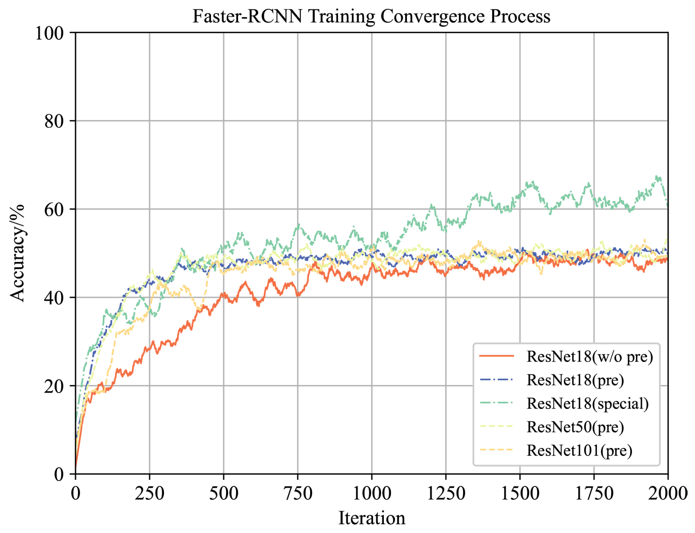
Faster-RCNN: We conduct a comparative analysis of Faster-RCNN using different backbone networks. Specifically, we examine ResNet18 (without pre-training, ImageNet pre-training, special pre-training), ResNet50 (ImageNet pre-training), and ResNet101 (ImageNet pre-training) to validate the effectiveness of our proposed Theorems 1 and 2, as well as the pre-training method. The initial learning rate is set at 0.001, decaying by 0.1 every 10 epochs. The training process consists of 20 epochs, with 100 iterations per epoch and a batch size of 6. We use the hybrid loss function from the original Faster-RCNN, depicted in Equation (
A9).
where
denotes the total Faster-RCNN loss,
denotes the classification loss,
denotes bounding box regression loss,
denotes the object loss, and
denotes the region proposal network bounding box regression loss. The convergence results of recognition accuracy are visually presented in
Figure A6.
Figure A6.
Training converegence process for Faster-RCNN.
Figure A6.
Training converegence process for Faster-RCNN.
YOLO: We employ the widely recognized YOLO-v5 for end-to-end recognition, implementing the YOLO-v5 algorithm across three specifications: v5s, v5m, and v5l. The training initiates with a learning rate of 0.001, with a decay rate of 0.1 every 10 epochs. Training spans 20 epochs, each consisting of 100 iterations, with a batch size of 12. The classical mixing loss function of YOLO is utilized, as depicted in Equation (
A10).
where
denotes the total YOLO loss,
denotes the object bounding box loss,
denotes the object mask loss, and
denotes the classification loss. In the experiment,
a,
b, and
c are set to 0.05, 1, and 0.5, respectively. The convergence outcomes regarding recognition accuracy across three distinct scales of YOLO-v5 networks are illustrated in
Figure A7.
Figure A7.
Training converegence process for YOLO.
Figure A7.
Training converegence process for YOLO.
DETR: During DETR training, an initial learning rate of 0.001 is set, with a decay rate of 0.1 every 10 epochs. Training spans 20 epochs, each consisting of 50 iterations, with a batch size of 64. In this configuration, the hidden layer of the transformer is established at 256 units, employing a total of six layers for both the transformer encoder and decoder. Additionally, multi-head attention utilizes eight heads in its operation. We employ the mixed loss and Adam optimizer as proposed in the original DETR paper, utilizing the mixed loss and weight outlined in Equation (
A11).
where
denotes the total DETR loss,
denotes the classification loss,
denotes the bounding box regression loss, and
denotes the GIOU loss. In the experiment,
,
, and
are set to 1, 5, and 2, respectively. Five distinct groups of independent experiments were conducted using various Backbone networks: ResNet18 (without pre-training, ImageNet pre-training, special pre-training), ResNet50 (ImageNet pre-training), and ResNet101 (ImageNet pre-training). The convergence results of recognition accuracy are visually presented in
Figure A8.
Figure A8.
Training converegence process for DETR.
Figure A8.
Training converegence process for DETR.


