
Ensemble Learning-Based Alzheimer’s Disease Classification Using Electroencephalogram Signals and Clock Drawing Test Images


Abstract
Highlights
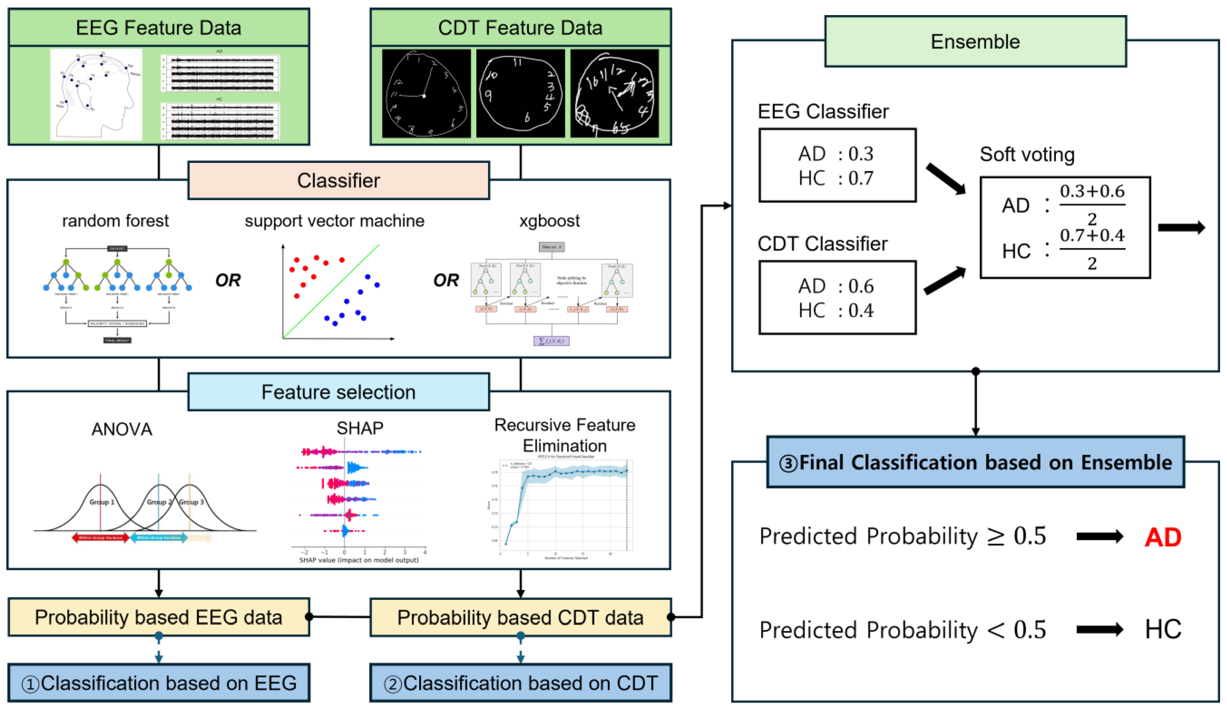
- Ensembles of probability-based electroencephalogram and clock drawing test data from Alzheimer’s disease patients outperform conventional machine learning techniques in terms of disease detection accuracy.
Abstract
1. Introduction
2. Materials and Methods
2.1. Data Collection
2.1.1. Materials
2.1.2. Electronic Medical Record (EMR) Data Collection
2.2. Data Preprocessing
2.2.1. EEG Signal Preprocessing
- Removal of transient noise introduced by movements during EEG measurement.
- Elimination of typical noise continuously introduced, based on frequency spectrum and topomap analysis.
- Exclusion of cases where the length of data extracted through the EEG refinement tool is less than 30 s, as it is difficult to ensure representativeness of individual resting-state EEG in such cases.
2.2.2. CDT Image Preprocessing
- Sending the test results conducted with the CDT application at each institution to the server.
- Image and video generation from the transmitted .json files.
- Extraction of the CDT performance timeline and coordinate values from the CDT app, and performance videos creation based on the timeline and coordinate values.
- Exclusion of some collected data if the timeline and coordinate values do not meet inclusion criteria.
2.3. Feature Extraction and Selection
2.4. Machine Learning and Classification
3. Results
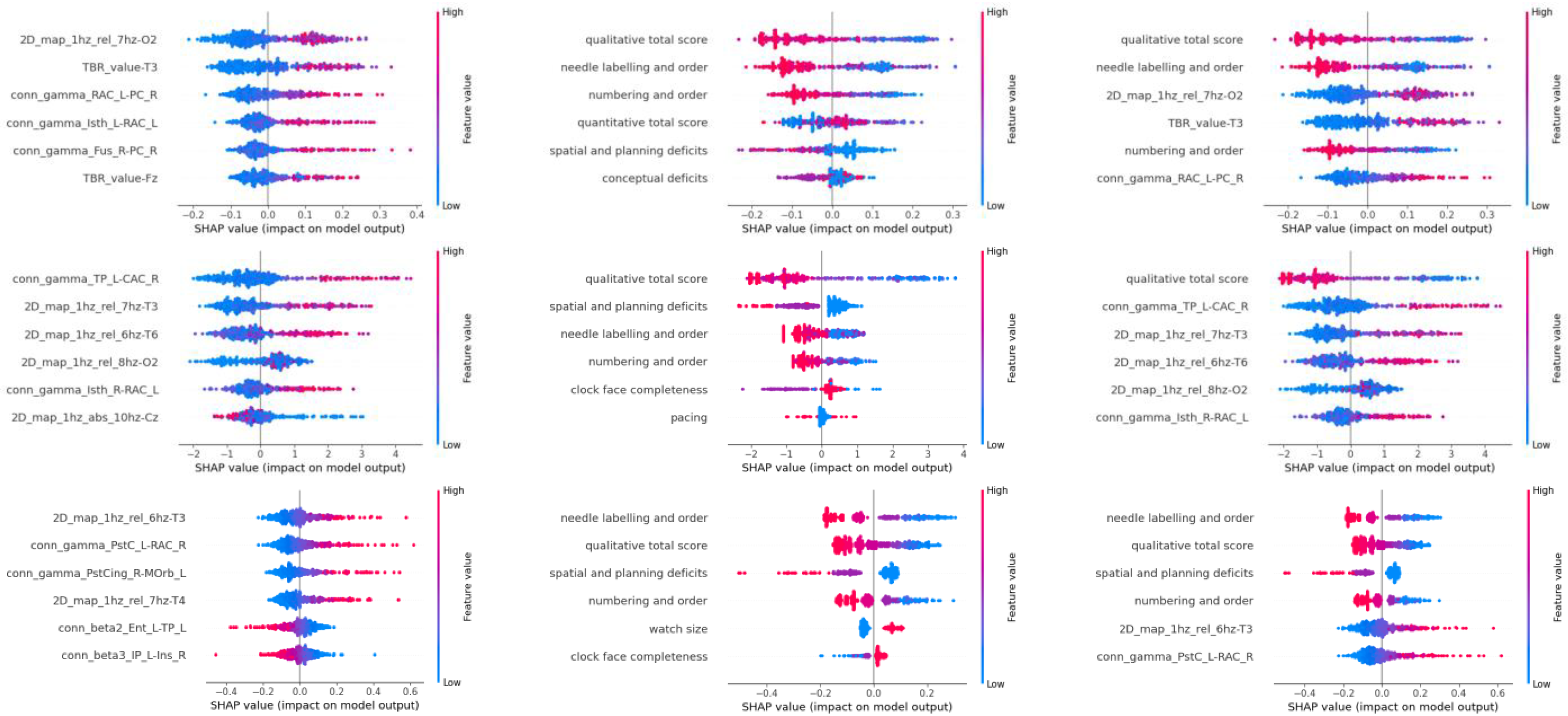
- For RF: The relative average value of the 7 Hz frequency band in the 2D map of the O2 electrode (2D_map_1hz_rel_7hz-O2);
- For XGB: The functional connectivity in the gamma wave band between the right Caudal Anterior Cingulate and left Temporal Pole (conn_gamma_TP_L-CAC_R);
- For SVM: The relative average value of the 6 Hz frequency band in the T3 electrode (2D_map_1hz_rel_6hz-T3).
4. Discussion
4.1. Role and Strength of Ensemble Methods in the Alzheimer’s Disease Classification Task
4.2. Appropriateness of Machine Learning Models Chosen for Training on EEG and CDT Data
4.3. Role of Analysis of Variance (ANOVA) in Feature Selection
4.4. Other Strengths and Limitations
Author Contributions
Funding
Institutional Review Board Statement
Informed Consent Statement
Data Availability Statement
Conflicts of Interest
Abbreviations
| AD | Alzheimer’s Disease |
| ANOVA | Analysis of Variance |
| CDT | Clock Drawing Test |
| CNN | Convolutional Neural Network |
| DNN | Deep Neural Network |
| EEG | Electroencephalogram |
| EL | Ensemble Learning |
| HC | Healthy Control (Normal) |
| MCI | Mild Cognitive Impairment |
| ML | Machine Learning |
| RF | Random Forest |
| RFE | Recursive Feature Elimination |
| SVM | Support Vector Machine |
| VIF | Variance Inflation Factor |
| XGB | eXtreme Gradient Boosting |
References
- Juganavar, A.; Joshi, A.; Shegekar, T. Navigating Early Alzheimer’s Diagnosis: A Comprehensive Review of Diagnostic Innovations. Cureus 2023, 15, e44937. [Google Scholar] [CrossRef] [PubMed]
- Division, U.P. World Population Ageing: 1950–2050; United Nations Digital Library: New York, NY, USA, 2002. [Google Scholar]
- Centers for Disease Control and Prevention. Public health and aging: Trends in aging--United States and worldwide. JAMA 2003, 289, 1371–1373. [Google Scholar] [CrossRef]
- Alzheimer’s Association. 2024 Alzheimer’s disease facts and figures. Alzheimers Dement. 2024, 20, 3708–3821. [Google Scholar] [CrossRef] [PubMed]
- Rajan, K.B.; Weuve, J.; Barnes, L.L.; McAninch, E.A.; Wilson, R.S.; Evans, D.A. Population estimate of people with clinical Alzheimer’s disease and mild cognitive impairment in the United States (2020–2060). Alzheimers Dement. 2021, 17, 1966–1975. [Google Scholar] [CrossRef] [PubMed]
- Kim, N.H.; Park, U.; Yang, D.W.; Choi, S.H.; Youn, Y.C.; Kang, S.W. PET-validated EEG-machine learning algorithm predicts brain amyloid pathology in pre-dementia Alzheimer’s disease. Sci. Rep. 2023, 13, 10299. [Google Scholar] [CrossRef]
- Ieracitano, C.; Mammone, N.; Bramanti, A.; Hussain, A.; Morabito, F.C. A Convolutional Neural Network approach for classification of dementia stages based on 2D-spectral representation of EEG recordings. Neurocomputing 2019, 323, 96–107. [Google Scholar] [CrossRef]
- Safi, M.S.; Safi, S.M.M. Early detection of Alzheimer’s disease from EEG signals using Hjorth parameters. Biomed. Signal Proces. 2021, 65, 102338. [Google Scholar] [CrossRef]
- Chen, S.; Stromer, D.; Alabdalrahim, H.A.; Schwab, S.; Weih, M.; Maier, A. Automatic dementia screening and scoring by applying deep learning on clock-drawing tests. Sci. Rep. 2020, 10, 20854. [Google Scholar] [CrossRef]
- Sato, K.; Niimi, Y.; Mano, T.; Iwata, A.; Iwatsubo, T. Automated Evaluation of Conventional Clock-Drawing Test Using Deep Neural Network: Potential as a Mass Screening Tool to Detect Individuals With Cognitive Decline. Front. Neurol. 2022, 13, 896403. [Google Scholar] [CrossRef]
- Nanni, L.; Lumini, A.; Zaffonato, N. Ensemble based on static classifier selection for automated diagnosis of Mild Cognitive Impairment. J. Neurosci. Methods 2018, 302, 42–46. [Google Scholar] [CrossRef]
- Chatterjee, S.; Byun, Y.C. Voting Ensemble Approach for Enhancing Alzheimer’s Disease Classification. Sensors 2022, 22, 7661. [Google Scholar] [CrossRef] [PubMed]
- An, N.; Ding, H.; Yang, J.; Au, R.; Ang, T.F.A. Deep ensemble learning for Alzheimer’s disease classification. J. Biomed. Inform. 2020, 105, 103411. [Google Scholar] [CrossRef] [PubMed]
- Huang, F.; Qiu, A. Ensemble Vision Transformer for Dementia Diagnosis. IEEE J. Biomed. Health Inform. 2024, 28, 5551–5561. [Google Scholar] [CrossRef] [PubMed]
- Hosseini, M.P.; Hosseini, A.; Ahi, K. A Review on Machine Learning for EEG Signal Processing in Bioengineering. IEEE Rev. Biomed. Eng. 2021, 14, 204–218. [Google Scholar] [CrossRef]
- Mahajan, P.; Uddin, S.; Hajati, F.; Moni, M.A. Ensemble Learning for Disease Prediction: A Review. Healthcare 2023, 11, 1808. [Google Scholar] [CrossRef]
- Yu, W.Y.; Sun, T.H.; Hsu, K.C.; Wang, C.C.; Chien, S.Y.; Tsai, C.H.; Yang, Y.W. Comparative analysis of machine learning algorithms for Alzheimer’s disease classification using EEG signals and genetic information. Comput. Biol. Med. 2024, 176, 108621. [Google Scholar] [CrossRef]
- Kivimaki, M.; Luukkonen, R.; Batty, G.D.; Ferrie, J.E.; Pentti, J.; Nyberg, S.T.; Shipley, M.J.; Alfredsson, L.; Fransson, E.I.; Goldberg, M.; et al. Body mass index and risk of dementia: Analysis of individual-level data from 1.3 million individuals. Alzheimers Dement. 2018, 14, 601–609. [Google Scholar] [CrossRef]
- Breiman, L. Random forests. Mach. Learn. 2001, 45, 5–32. [Google Scholar] [CrossRef]
- Chen, T.; Guestrin, C. XGBoost. In Proceedings of the 22nd ACM SIGKDD International Conference on Knowledge Discovery and Data Mining, San Francisco, CA, USA, 13–17 August 2016; pp. 785–794. [Google Scholar]
- Valkenborg, D.; Rousseau, A.J.; Geubbelmans, M.; Burzykowski, T. Support vector machines. Am. J. Orthod. Dentofacial Orthop. 2023, 164, 754–757. [Google Scholar] [CrossRef]
- Wei, L.; Ventura, S.; Lowery, M.; Ryan, M.A.; Mathieson, S.; Boylan, G.B.; Mooney, C. Random Forest-based Algorithm for Sleep Spindle Detection in Infant EEG. Annu. Int. Conf. IEEE Eng. Med. Biol. Soc. 2020, 2020, 58–61. [Google Scholar] [CrossRef]
- Kamarajan, C.; Ardekani, B.A.; Pandey, A.K.; Chorlian, D.B.; Kinreich, S.; Pandey, G.; Meyers, J.L.; Zhang, J.; Kuang, W.; Stimus, A.T.; et al. Random Forest Classification of Alcohol Use Disorder Using EEG Source Functional Connectivity, Neuropsychological Functioning, and Impulsivity Measures. Behav. Sci. 2020, 10, 62. [Google Scholar] [CrossRef]
- Davoudi, A.; Dion, C.; Amini, S.; Tighe, P.J.; Price, C.C.; Libon, D.J.; Rashidi, P. Classifying Non-Dementia and Alzheimer’s Disease/Vascular Dementia Patients Using Kinematic, Time-Based, and Visuospatial Parameters: The Digital Clock Drawing Test. J. Alzheimers Dis. 2021, 82, 47–57. [Google Scholar] [CrossRef]
- Escobar-Ipuz, F.A.; Torres, A.M.; García-Jiménez, M.A.; Basar, C.; Cascón, J.; Mateo, J. Prediction of patients with idiopathic generalized epilepsy from healthy controls using machine learning from scalp EEG recordings. Brain Res. 2023, 1798, 148131. [Google Scholar] [CrossRef] [PubMed]
- Yu, W.; Liu, T.; Valdez, R.; Gwinn, M.; Khoury, M.J. Application of support vector machine modeling for prediction of common diseases: The case of diabetes and pre-diabetes. BMC Med. Inform. Decis. Mak. 2010, 10, 16. [Google Scholar] [CrossRef]
- Kim, H.; Yoshimura, N.; Koike, Y. Classification of Movement Intention Using Independent Components of Premovement EEG. Front. Hum. Neurosci. 2019, 13, 63. [Google Scholar] [CrossRef] [PubMed]
- Ma, Y.; Ding, X.; She, Q.; Luo, Z.; Potter, T.; Zhang, Y. Classification of Motor Imagery EEG Signals with Support Vector Machines and Particle Swarm Optimization. Comput. Math. Methods Med. 2016, 2016, 4941235. [Google Scholar] [CrossRef]
- Masuo, A.; Ito, Y.; Kanaiwa, T.; Naito, K.; Sakuma, T.; Kato, S. Dementia Screening Based on SVM Using Qualitative Drawing Error of Clock Drawing Test. In Proceedings of the 2022 44th Annual International Conference of the IEEE Engineering in Medicine & Biology Society (EMBC), Glasgow, UK, 11–15 July 2022; pp. 4484–4487. [Google Scholar] [CrossRef]
- Tripathy, G.; Sharaff, A. AEGA: Enhanced feature selection based on ANOVA and extended genetic algorithm for online customer review analysis. J. Supercomput. 2023, 79, 13180–13209. [Google Scholar] [CrossRef] [PubMed]
- Ding, H.; Feng, P.-M.; Chen, W.; Lin, H. Identification of bacteriophage virion proteins by the ANOVA feature selection and analysis. Mol. Biosyst. 2014, 10, 2229–2235. [Google Scholar] [CrossRef]
- Wang, Y.H.; Zhang, Y.F.; Zhang, Y.; Gu, Z.F.; Zhang, Z.Y.; Lin, H.; Deng, K.J. Identification of adaptor proteins using the ANOVA feature selection technique. Methods 2022, 208, 42–47. [Google Scholar] [CrossRef]
- Guyon, I.; Weston, J.; Barnhill, S.; Vapnik, V. Gene Selection for Cancer Classification using Support Vector Machines. Mach. Learn. 2002, 46, 389–422. [Google Scholar] [CrossRef]
- Ponce-Bobadilla, A.V.; Schmitt, V.; Maier, C.S.; Mensing, S.; Stodtmann, S. Practical guide to SHAP analysis: Explaining supervised machine learning model predictions in drug development. Clin. Transl. Sci. 2024, 17, e70056. [Google Scholar] [CrossRef]
- Shim, Y.; Yang, D.W.; Ho, S.; Hong, Y.J.; Jeong, J.H.; Park, K.H.; Kim, S.; Wang, M.J.; Choi, S.H.; Kang, S.W. Electroencephalography for Early Detection of Alzheimer’s Disease in Subjective Cognitive Decline. Dement. Neurocogn Disord. 2022, 21, 126–137. [Google Scholar] [CrossRef]
- Zheng, X.; Wang, B.; Liu, H.; Wu, W.; Sun, J.; Fang, W.; Jiang, R.; Hu, Y.; Jin, C.; Wei, X.; et al. Diagnosis of Alzheimer’s disease via resting-state EEG: Integration of spectrum, complexity, and synchronization signal features. Front. Aging Neurosci. 2023, 15, 1288295. [Google Scholar] [CrossRef]
- Rasheed, K.; Qayyum, A.; Qadir, J.; Sivathamboo, S.; Kwan, P.; Kuhlmann, L.; O’Brien, T.; Razi, A. Machine Learning for Predicting Epileptic Seizures Using EEG Signals: A Review. IEEE Rev. Biomed. Eng. 2021, 14, 139–155. [Google Scholar] [CrossRef] [PubMed]
- Vicchietti, M.L.; Ramos, F.M.; Betting, L.E.; Campanharo, A.S.L.O. Computational methods of EEG signals analysis for Alzheimer’s disease classification. Sci. Rep. 2023, 13, 8184. [Google Scholar] [CrossRef] [PubMed]
- Akbar, F.; Taj, I.; Usman, S.M.; Imran, A.S.; Khalid, S.; Ihsan, I.; Ali, A.; Yasin, A. Unlocking the potential of EEG in Alzheimer’s disease research: Current status and pathways to precision detection. Brain Res. Bull. 2025, 223, 111281. [Google Scholar] [CrossRef] [PubMed]
- Spenciere, B.; Alves, H.; Charchat-Fichman, H. Scoring systems for the Clock Drawing Test: A historical review. Dement. Neuropsychol. 2017, 11, 6–14. [Google Scholar] [CrossRef] [PubMed]
- Singh, S.G.; Das, D.; Barman, U.; Saikia, M.J. Early Alzheimer’s Disease Detection: A Review of Machine Learning Techniques for Forecasting Transition from Mild Cognitive Impairment. Diagnostics 2024, 14, 1759. [Google Scholar] [CrossRef]
- Qiu, S.; Miller, M.I.; Joshi, P.S.; Lee, J.C.; Xue, C.; Ni, Y.; Wang, Y.; De Anda-Duran, I.; Hwang, P.H.; Cramer, J.A.; et al. Multimodal deep learning for Alzheimer’s disease dementia assessment. Nat. Commun. 2022, 13, 3404. [Google Scholar] [CrossRef]
- Rodinskaia, D.; Radinski, C.; Labuhn, J. EEG coherence as a marker of functional connectivity disruption in Alzheimer’s disease. Aging Health Res. 2022, 2, 100098. [Google Scholar] [CrossRef]
- Chetty, C.A.; Bhardwaj, H.; Kumar, G.P.; Devanand, T.; Sekhar, C.S.A.; Akturk, T.; Kiyi, I.; Yener, G.; Guntekin, B.; Joseph, J.; et al. EEG biomarkers in Alzheimer’s and prodromal Alzheimer’s: A comprehensive analysis of spectral and connectivity features. Alzheimers Res. Ther. 2024, 16, 236. [Google Scholar] [CrossRef]
- Masuo, A.; Kubota, J.; Yokoyama, K.; Karaki, K.; Yuasa, H.; Ito, Y.; Takeo, J.; Sakuma, T.; Kato, S. Machine learning-based screening for outpatients with dementia using drawing features from the clock drawing test. Clin. Neuropsychol. 2024; online ahead of print. [Google Scholar] [CrossRef] [PubMed]
- Sarica, A.; Cerasa, A.; Quattrone, A. Random Forest Algorithm for the Classification of Neuroimaging Data in Alzheimer’s Disease: A Systematic Review. Front. Aging Neurosci. 2017, 9, 329. [Google Scholar] [CrossRef]
- Khan, M.S.; Salsabil, N.; Alam, M.G.R.; Dewan, M.A.A.; Uddin, M.Z. CNN-XGBoost fusion-based affective state recognition using EEG spectrogram image analysis. Sci. Rep. 2022, 12, 14122. [Google Scholar] [CrossRef] [PubMed]
- Chen, W.; Lei, X.; Chakrabortty, R.; Chandra Pal, S.; Sahana, M.; Janizadeh, S. Evaluation of different boosting ensemble machine learning models and novel deep learning and boosting framework for head-cut gully erosion susceptibility. J. Environ. Manage 2021, 284, 112015. [Google Scholar] [CrossRef] [PubMed]
- Cherif, I.L.; Kortebi, A. On using eXtreme Gradient Boosting (XGBoost) Machine Learning algorithm for Home Network Traffic Classification. In Proceedings of the 2019 Wireless Days (WD), Manchester, UK, 24–26 April 2019; pp. 1–6. [Google Scholar]
- Yuan, S.; Sun, Y.; Xiao, X.; Long, Y.; He, H. Using Machine Learning Algorithms to Predict Candidaemia in ICU Patients With New-Onset Systemic Inflammatory Response Syndrome. Front Med. 2021, 8, 720926. [Google Scholar] [CrossRef]
- Tunc, H.C.; Sakar, C.O.; Apaydin, H.; Serbes, G.; Gunduz, A.; Tutuncu, M.; Gurgen, F. Estimation of Parkinson’s disease severity using speech features and extreme gradient boosting. Med. Biol. Eng. Comput. 2020, 58, 2757–2773. [Google Scholar] [CrossRef]
- Lee, M.; Yeo, N.Y.; Ahn, H.J.; Lim, J.S.; Kim, Y.; Lee, S.H.; Oh, M.S.; Lee, B.C.; Yu, K.H.; Kim, C. Prediction of post-stroke cognitive impairment after acute ischemic stroke using machine learning. Alzheimers Res. Ther. 2023, 15, 147. [Google Scholar] [CrossRef]
- Cortes, C.; Vapnik, V. Support-vector networks. Mach. Learn. 1995, 20, 273–297. [Google Scholar] [CrossRef]
- Barghout, L. Spatial-Taxon Information Granules as Used in Iterative Fuzzy-Decision-Making for Image Segmentation. In Granular Computing and Decision-Making: Interactive and Iterative Approaches; Pedrycz, W., Chen, S.-M., Eds.; Springer International Publishing: Cham, Switzerland, 2015; pp. 285–318. [Google Scholar]
- Decoste, D.; Schölkopf, B. Training Invariant Support Vector Machines. Mach. Learn. 2002, 46, 161–190. [Google Scholar] [CrossRef]
- Maitra, D.S.; Bhattacharya, U.; Parui, S.K. CNN based common approach to handwritten character recognition of multiple scripts. In Proceedings of the 2015 13th International Conference on Document Analysis and Recognition (ICDAR), Tunis, Tunisia, 23–26 August 2015; pp. 1021–1025. [Google Scholar]
- Kim, H.; Yoshimura, N.; Koike, Y. Characteristics of Kinematic Parameters in Decoding Intended Reaching Movements Using Electroencephalography (EEG). Front. Neurosci. 2019, 13, 1148. [Google Scholar] [CrossRef] [PubMed]
- Fastame, M.C.; Mulas, I.; Putzu, V.; Asoni, G.; Viale, D.; Mameli, I.; Pau, M. The contribution of motor efficiency to drawing performance of older people with and without signs of cognitive decline. Appl. Neuropsychol. Adult 2023, 30, 360–367. [Google Scholar] [CrossRef] [PubMed]


| Classes | Train | Test | Total |
|---|---|---|---|
| Alzheimer’s Disease | 160 (159) | 39 (40) | 199 |
| Healthy Control | 160 | 40 | 200 |
| Data | Rank | RF | XGB | SVM |
|---|---|---|---|---|
| EEG | 1 | 2D_map_1hz_rel_7hz-O2 | conn_gamma_TP_L-CAC_R | 2D_map_1hz_rel_6hz-T3 |
| 2 | TBR_value-T3 | 2D_map_1hz_rel_7hz | conn_gamma_PstC_L-RAC_R | |
| 3 | conn_gamma_RAC_L-PC_R | 2D_map_1hz_rel_6hz-T6 | conn_gamma_PstCing_R-MOrb_L | |
| 4 | conn_gamma_lsth_L-RAC_L | 2D_map_1hz_rel_8hz-O2 | 2D_map_1hz_rel_7hz-T4 | |
| 5 | conn_gamma_Fus_R-PC_R | conn_gamma_lsth_R-RAC_L | conn_beta2_Ent_L-TP_L | |
| 6 | TBR_value_Fz | 2D_map_1hz_abs_10hz-Cz | conn_beta3_IP_L-Ins_R | |
| CDT | 1 | Qualitative Total Score | Qualitative Total Score | Needle Labeling and Order |
| 2 | Needle Labeling and Order | Spatial and Planning Deficits | Qualitative Total Score | |
| 3 | Numbering and Order | Needle Labeling and Order | Spatial and Planning Deficits | |
| 4 | Quantitative Total Score | Numbering and Order | Numbering and Order | |
| 5 | Spatial and Planning Deficits | Clock Face Completeness | Watch Size | |
| 6 | Conceptual Deficits | Pacing | Clock Face Completeness |
| Classifier | Metrics | EEG | CDT | Ensembles |
|---|---|---|---|---|
| RF | Precision | 0.800 (±0.059) | 0.853 (±0.043) | 0.865 (±0.031) |
| Recall | 0.737 (±0.051) | 0.702 (±0.110) | 0.758 (±0.055) | |
| F1-Score | 0.766 (±0.052) | 0.740 (±0.071) | 0.798 (±0.036) | |
| Accuracy | 0.776 (±0.051) | 0.759 (±0.053) | 0.809 (±0.031) | |
| XGB | Precision | 0.848 (±0.042) | 0.875 (±0.044) | 0.917 (±0.049) |
| Recall | 0.773 (±0.059) | 0.692 (±0.081) | 0.859 (±0.041) | |
| F1-Score | 0.786 (±0.035) | 0.749 (±0.041) | 0.863 (±0.038) | |
| Accuracy | 0.791 (±0.032) | 0.771 (±0.029) | 0.864 (±0.039) | |
| SVM | Precision | 0.909 (±0.072) | 0.824 (±0.053) | 0.972 (±0.085) |
| Recall | 0.763 (±0.037) | 0.708 (±0.134) | 0.824 (±0.069) | |
| F1-Score | 0.806 (±0.045) | 0.754 (±0.083) | 0.850 (±0.052) | |
| Accuracy | 0.817 (±0.046) | 0.777 (±0.061) | 0.854 (±0.054) |
| RF | XGB | SVM | |
|---|---|---|---|
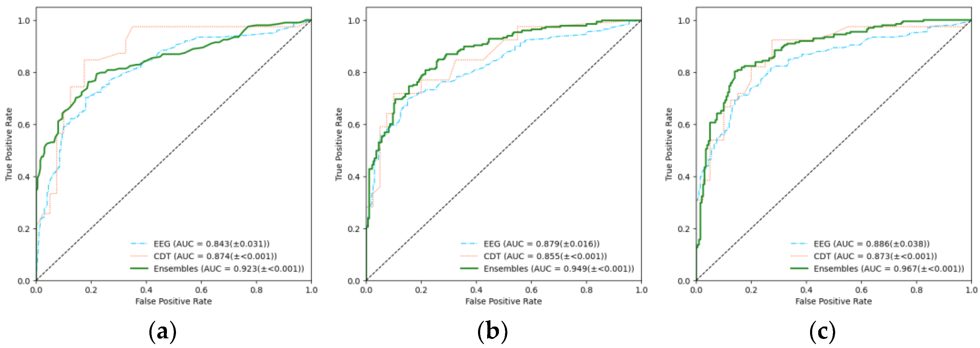
| EEG | 0.843 (±0.031) | 0.879 (±0.016) | 0.886 (±0.038) |
| CDT | 0.874 (±<0.001) | 0.855 (±<0.001) | 0.873 (±<0.001) |
| Ensemble (EEG+CDT) | 0.923 (±<0.001) | 0.949 (±<0.001) | 0.967 (±<0.001) |
| Model Comparison | p-Value | Statistical Significance (α = 0.016) |
|---|---|---|
| RF vs. SVM | 0.0019 | Significant difference |
| RF vs. XGB | 0.0019 | Significant difference |
| SVM vs. XGB | 0.2200 | No significant difference |
Disclaimer/Publisher’s Note: The statements, opinions and data contained in all publications are solely those of the individual author(s) and contributor(s) and not of MDPI and/or the editor(s). MDPI and/or the editor(s) disclaim responsibility for any injury to people or property resulting from any ideas, methods, instructions or products referred to in the content. |
© 2025 by the authors. Licensee MDPI, Basel, Switzerland. This article is an open access article distributed under the terms and conditions of the Creative Commons Attribution (CC BY) license (https://creativecommons.org/licenses/by/4.0/).
Share and Cite
Huh, Y.J.; Park, J.-h.; Kim, Y.J.; Kim, K.G. Ensemble Learning-Based Alzheimer’s Disease Classification Using Electroencephalogram Signals and Clock Drawing Test Images. Sensors 2025, 25, 2881. https://doi.org/10.3390/s25092881
Huh YJ, Park J-h, Kim YJ, Kim KG. Ensemble Learning-Based Alzheimer’s Disease Classification Using Electroencephalogram Signals and Clock Drawing Test Images. Sensors. 2025; 25(9):2881. https://doi.org/10.3390/s25092881
Chicago/Turabian StyleHuh, Young Jae, Jun-ha Park, Young Jae Kim, and Kwang Gi Kim. 2025. "Ensemble Learning-Based Alzheimer’s Disease Classification Using Electroencephalogram Signals and Clock Drawing Test Images" Sensors 25, no. 9: 2881. https://doi.org/10.3390/s25092881
APA StyleHuh, Y. J., Park, J.-h., Kim, Y. J., & Kim, K. G. (2025). Ensemble Learning-Based Alzheimer’s Disease Classification Using Electroencephalogram Signals and Clock Drawing Test Images. Sensors, 25(9), 2881. https://doi.org/10.3390/s25092881