Non-Fragile Estimation for Nonlinear Delayed Complex Networks with Random Couplings Using Binary Encoding Schemes

Abstract

This paper is dedicated to dealing with the design issue of a non-fragile state estimator for a type of nonlinear complex network subject to random couplings and random multiple time delays under binary encoding schemes (BESs). The BESs are put into use in the transmission of data from the sensor to the remote estimator. The phenomenon of bit errors is considered in the process of signal transmission, whose description utilizes a Bernoulli-distributed random sequence. The random couplings are represented by using the Kronecker delta function as well as a Markov chain. This paper aims to conduct a non-fragile state estimation such that, in the presence of some variations/perturbations in the gain parameter of the estimator, the estimation error dynamics will reach exponential ultimate boundedness in mean square and the ultimate bound will be minimized. Utilizing both stochastic analysis and matrix inequality processing, a sufficient condition is provided to guarantee that the constructed estimator satisfies the expected estimation performance, and the estimator gains are acquired by tackling an optimization issue constrained by some linear matrix inequalities. Eventually, two simulation examples are conducted, whose results verify that the approach to the design of a non-fragile estimator in this paper is effective.

1. Introduction

Complex networks (CNs) are large-scale networked systems comprising numerous network nodes, which are distributed and connected in terms of a specific coupling structure [1,2,3,4]. CNs have attracted sustained interest from researchers in the field of systems and control due to their remarkable description/abstraction ability in numerous practical networks, including gene networks, power grids, transport networks, and artificial neural networks, and some representative results are provided in the references [5,6,7,8,9]. In the last decade, there has been a large body of research dedicated to investigating the issues in the dynamic analysis of CNs, including synchronization issues [10,11], stability analyses issues [12,13], state estimation (SE) issues [14,15], and others. It is important to highlight that studying CNs requires access to state information within the various nodes. However, measuring the network state directly from the sensor output measurements can pose challenges, especially in large-scale networks where information may be incomplete. Hence, the issues in SE for CNs, including variance-constrained SE, non-fragile SE, $H_{\infty }$ SE, minimum-variance SE, and recursive SE [16,17,18,19,20], have attracted a substantial amount of attention. For example, the variance-constrained SE problem has been investigated in [16] for a class of CNs involving quantized measurements and uncertain inner coupling. In [19], the randomly occurring sensor saturations were the focus, and a non-fragile state estimator of CNs was designed based on a dynamic event-triggering mechanism.

In practical networked control systems (NCSs), constraint phenomena inevitably occur due to the limited bandwidth, sensor failures, and complex operating environments, which may include system constraints (nonlinearity, time-delays, input saturation, and noise), measurement constraints (sensor saturation and sensor faults), and communication constraints (cyber attacks and channel fadings) [21,22,23,24,25,26,27,28]. The overall performance of CNs may be impacted more significantly by the constraint phenomena due to their intricate structure, which includes a topology of different network nodes and a coupling structure within a single node [29,30]. It is widely recognized that the outer coupling of a CN reflects the topology linkage among neighboring nodes, and the inner coupling depicts the intensity of the internal connections in an individual node. However, the coupling matrices are sometimes variable or unknown due to possible errors in modeling CNs, component aging, and changing working conditions [31]. Although the complexity of the coupling matrix makes it harder to analyze the dynamics of CNs, it is essential to take account of the impact of random couplings while analyzing the dynamic behavior of CNs. Research on constraint phenomena in CNs has received increasing interest [32,33,34]. For instance, the phenomena of uncertain inner coupling, sensor saturation, quantization, and missing measurements were contemplated regarding the SE problem for CNs in [34]. Due to the inadequate research results obtained, it is meaningful to conduct in-depth studies on the SE issue for CNs using random couplings, which is an objective of this paper.

For NCSs, communication transmission often takes up a large number of network resources, and the transmission data may be stolen by cyber hackers; thus, reducing the consumption of network resources in the communication process and ensuring the security of the data being communicated has become an urgent need. Compared to information transmission using analog signals among NCSs devices, communicating in a digital way has benefits including powerful resistance to noise disturbances, the high reliability of data transmission, and high confidentiality [35,36,37,38,39,40,41]. To date, various communication schemes have been adopted to decrease the consumption of communication resources, such as the communication protocol [42,43,44,45,46,47] and the event-triggering strategy [48,49,50]. Most existing data transmission strategies aim to alleviate the congestions and conflicts associated with transmission by reducing the communication traffic in the transmission channels or the frequency of data transmission.

In recent years, another communication mechanism has been widely studied, i.e., the encoding–decoding scheme [51,52,53,54], where the binary encoding scheme (BES), a traditional method, has been applied in the SE issue of NCSs [15,55,56]. The core idea of the BESs is to encode the data through a binary encoder as a binary bit string (BBS), which is to be transmitted via a binary symmetric channel (BSC) and then decoded by a binary decoder at the receiving end of the data. The use of BESs for transmission has allowed for data compression, reduced the communication bandwidth to an extent, and enhanced the security of data communication. Despite these advantages, distortion also occurs during data transmission using BESs. During the transmission of the BBS through a BSC, bit flipping inevitably occurs to a binary bit due to the presence of channel noise, e.g., a change from 0 to 1 or a change from 1 to 0. This phenomenon is also known as the bit error, which brings additional challenges to the analysis of CNs dynamics. If not dealt with properly when conducting the analysis, bit error may have a negative effect on both the correctness of data transmission and, inevitably, the estimator performance [15,56,57,58]; furthermore, investigations into the estimation of CNs using BESs have only recently become the subject of research. Hence, another objective of this paper was to study the SE issue for CNs using BESs while analyzing the impact of random bit errors on the estimator performance.

As is known, non-fragile SE issues with NCSs typically arise regarding the possible occurrence of fluctuations in gain in the actual execution course, which are caused by working environment effects or abrupt changes. In most of the literature on SE for CNs, the results were obtained by assuming that the constructed state estimators are accurate and realizable [59,60,61]. However, this assumption may be unrealistic for practical systems due to various factors interfering with the actual process, such as the aging of electronic components within the device or the inaccurate implementation of the digital system. That is, the implemented estimator gain parameters may deviate from the expected value to an unpredictable degree, which would sometimes cause severe estimation errors in the system. Therefore, the development of a non-fragile estimator that can resist these gain perturbations is necessary; this could involve including gain variations prior to estimation in the estimator model. At present, the non-fragile estimation issue is receiving increasing attention [19,62,63,64,65]. For instance, in [64], a $H_{\infty }$ non-fragile estimator was designed to deal with the fault estimation issue for a type of system with time-varying parameters over sensor networks. Nevertheless, non-fragile estimator designs for CNs have not been paid enough attention yet in which BESs, random couplings, and random multiple time delays are all taken into account simultaneously.

In response to these issues, our study aims to address the non-fragile SE problem for delayed CNs with randomly varying couplings under BESs. The crucial difficulties to be resolved through the developed non-fragile estimation strategy are as follows: (1) How can one characterize and describe the randomly varying couplings of CNs? (2) How can the influence from bit errors on SE performance be indicated? (3) How can a non-fragile estimator be devised that satisfies the exponential ultimate boundedness in mean squares? The highlights of this paper are emphasized as follows: (1) the non-fragile SE issue is effectively tackled in this paper for nonlinear CNs, which encompass randomly occurring multiple delays and randomly varying couplings under the BESs; (2) a sufficient condition is brought up, which is used to design the non-fragile estimator, guarantee the exponential ultimate boundedness of the SE error dynamics in mean square, and derive the minimized ultimate bound of the estimation error; and (3) the estimator gain parameters are acquired via tackling an optimization issue constrained by some linear matrix inequalities.

Notation: The symbol appearing in this paper is fairly normalised. ${\mathbb{R}}^n$ is the n-dimensional Euclidean space. $\parallel ·\parallel$ indicates the standard norm. For a square matrix A, $A^{-1}$, $\mathrm{tr}\left\{\mathrm{A}\right\}$, ${\phi }_{min}\left(A\right)$ (${\phi }_{max}\left(A\right)$), and $A>0$ $(A\ge 0)$ reveal the inverse of A, the trace of A, the minimum (maximum) eigenvalue of A, and A is positive-definite (positive semi-definite), respectively. $B^T$ means the transpose of matrix B. The symbol ⊗ expresses the Kronecker product. $I_{\left(n\right)}$ ($0_{(r\times o)}$) represents the identity (zero) matrix with the dimension $n\times n$ ($r\times o$). For a random variable/vector w, $\mathbb{V}\left\{w\right\}$ and $\mathbb{E}\left\{w\right\}$ symbolise its variance and expectation, respectively. $\mathrm{diag}\{\dots \}$ describes a diagonal matrix.

2. Problem Formulation and Preliminaries

2.1. The Mathematical Description of Network Nodes

A class of discrete-time delayed CNs with U nodes were used, as follows:

$$\begin{array}{cc}\hfill x_i(s+1)=& A_i{x}_i\left(s\right)+B_{\mathcal{b}i}\sum _{l=1}^m{϶}_{il}\left(s\right)x_i(s-{\mathcal{b}}_l\left(s\right))+E_{i}g\left(x_i\left(s\right)\right)\hfill \\ \hfill & +\sum _{\zeta =1}^p\sum _{j=1}^U\delta (\varkappa \left(s\right),\zeta )a_{ij}^{\left(\zeta \right)}{\mathrm{\Gamma }}^{\left(\zeta \right)}{x}_j\left(s\right)+F_i{w}_i\left(s\right)(i=1,2,\dots ,U)\hfill \end{array}$$

(1)

where $x_i\left(s\right)\in {\mathbb{R}}^{l_x}$ denotes the state vector of node i; $w_i\left(s\right)\in {\mathbb{R}}^{l_w}$ is the process noise depicted by a bounded stochastic noise sequence fulfilling $\mathbb{E}\left\{w_i\left(s\right)\right\}=0$ and $\mathbb{V}\left\{w_i\left(s\right)\right\}=w_0^2{I}_{\left(l_w\right)}$ with a scalar $w_0>0$; $A_i$, $B_{\mathcal{b}i}$, $E_i$ and $F_i$ are the given system parameters matrices with suitable dimensions; and ${\mathrm{\Lambda }}^{\left(\zeta \right)}={\left[a_{ij}^{\left(\zeta \right)}\right]}_{U\times U}(\zeta =1,2,\dots ,p)$ is the outer coupling configuration matrix of CN (1) with $a_{ij}^{\left(\zeta \right)}\ge 0$ ($i\ne j$) but not all zero. Generally, ${\mathrm{\Lambda }}^{\left(\zeta \right)}$ is symmetric (i.e., ${\mathrm{\Lambda }}^{\left(\zeta \right)}={\mathrm{\Lambda }}^{\left(\zeta \right)T}$ ) and satisfies

$$\begin{array}{c}\hfill \sum _{j=1}^U{a}_{ij}^{\left(\zeta \right)}=\sum _{j=1}^U{a}_{ji}^{\left(\zeta \right)}=0(i=1,2,\dots ,U,\zeta =1,2,\dots ,p).\end{array}$$

${\mathrm{\Gamma }}^{\left(\zeta \right)}=\mathrm{diag}\{{\alpha }_1^{\left(\zeta \right)},{\alpha }_2^{\left(\zeta \right)},\dots ,{\alpha }_{l_x}^{\left(\zeta \right)}\}\ge 0$ is the inner coupling matrix linking the ℏth $\left(\hslash =1,2,\dots ,l_x\right)$ state variable if ${\alpha }_{\hslash }\ne 0$; $\delta \left(\varkappa \right(s),\zeta )$ is the Kronecker delta function, as follows:

$$\begin{array}{c}\hfill \delta (\mathsf{ı},\wp )=\left\{\begin{array}{cc}1,& \mathrm{if}\mathsf{ı}=\wp \\ 0,& \mathrm{if}\mathsf{ı}\ne \wp .\end{array}\right.\end{array}$$

$\varkappa \left(s\right)$ is a stochastic variable that represents randomly varying couplings of CN (1), which conforms to a discrete-time homogeneous Markov chain with values in a finite state space, as follows:

$$\begin{array}{c}\hfill \mathit{\Im }=\{1,2,\dots ,p\}\end{array}$$

and $\mathrm{\Pi }={\left[{\pi }_{ab}\right]}_{p\times p}$ symbolises a transition probability matrix with elements denoted by

$$\begin{array}{c}\hfill {\pi }_{ab}=\mathrm{Prob}\{\varkappa (s+1)=b|\varkappa \left(s\right)=a\}.\end{array}$$

(2)

Assumption 1

([5]). $g(·)\in {\mathbb{R}}^{l_x}$ is a nonlinear vector-valued function with $g\left(0\right)=0$, which meets

$$\begin{array}{cc}\hfill & {[g\left(z_1\right)-g\left(z_2\right)-{\Xi }_1(z_1-z_2)]}^T[g\left(z_1\right)-g\left(z_2\right)-{\Xi }_2(z_1-z_2)]\le 0,\forall z_1,z_2\in {\mathbb{R}}^{l_x}.\hfill \end{array}$$

(3)

In the term ${\displaystyle \sum _{l=1}^m}{϶}_{il}\left(s\right)x_i(s-{\mathcal{b}}_l\left(s\right)),{\mathcal{b}}_l\left(s\right)(l=1,2,\dots ,m)$ characterizes the stochastic and time-varying essence of communication delays that meet the condition $0<\underline{\mathcal{b}}\le {\mathcal{b}}_l\left(s\right)\le \overline{\mathcal{b}}$, where $\underline{\mathcal{b}}$ and $\overline{\mathcal{b}}$ are known and stand for the lower and upper bounds of delays. ${϶}_{il}\left(s\right)$ is a random variable represented by a Bernoulli distribution, as follows:

$$\begin{array}{c}\hfill \mathrm{Prob}\{{϶}_{il}\left(s\right)=1\}={\overline{϶}}_{il},\mathrm{Prob}\{{϶}_{il}\left(s\right)=0\}=1-{\overline{϶}}_{il}.\end{array}$$

Denoting ${\widetilde{϶}}_{il}\left(s\right)\triangleq {϶}_{il}\left(s\right)-{\overline{϶}}_{il}$, we can obtain the following statistical properties:

$$\begin{array}{c}\hfill \mathbb{E}\left\{{({϶}_{il}\left(s\right)-{\overline{϶}}_{il})}^2\right\}=\mathbb{E}\left\{{\left({\widetilde{϶}}_{il}\left(s\right)\right)}^2\right\}={\overline{϶}}_{il}(1-{\overline{϶}}_{il}).\end{array}$$

Therefore, the dynamics of CN (1) can be rewritten as follows:

$$\begin{array}{cc}\hfill x_i(s+1)=& A_i{x}_i\left(s\right)+\sum _{\zeta =1}^p\sum _{j=1}^U\delta (\varkappa \left(s\right),\zeta )a_{ij}^{\left(\zeta \right)}{\mathrm{\Gamma }}^{\left(\zeta \right)}{x}_j\left(s\right)+B_{\mathcal{b}i}\sum _{l=1}^m{\widetilde{϶}}_{il}\left(s\right)x_i(s-{\mathcal{b}}_l\left(s\right))\hfill \\ \hfill & +B_{\mathcal{b}i}\sum _{l=1}^m{\overline{϶}}_{il}{x}_i(s-{\mathcal{b}}_l\left(s\right))+E_{i}g\left(x_i\left(s\right)\right)+F_i{w}_i\left(s\right).\hfill \end{array}$$

(4)

The measurement signal $y_i\left(s\right)$ from the ith node is given as follows:

$$\begin{array}{c}\hfill y_i\left(s\right)=C_i{x}_i\left(s\right)+D_i{v}_i\left(s\right)\end{array}$$

(5)

where $y_i\left(s\right)\in {\mathbb{R}}^{l_y}$ is the measurement output of the ith ($i=1,2,\dots ,U$) node, $C_i$ and $D_i$ represent known matrices with rational dimensions, and $v_i\left(s\right)\in {\mathbb{R}}^{l_v}$ is the measurement noise, which is a bounded stochastic noise sequence satisfying $\mathbb{E}\left\{v_i\left(s\right)\right\}=0$ and $\mathbb{V}\left\{v_i\left(s\right)\right\}=v_0^2{I}_{\left(l_v\right)}$, with $v_0$ being a positive scalar.

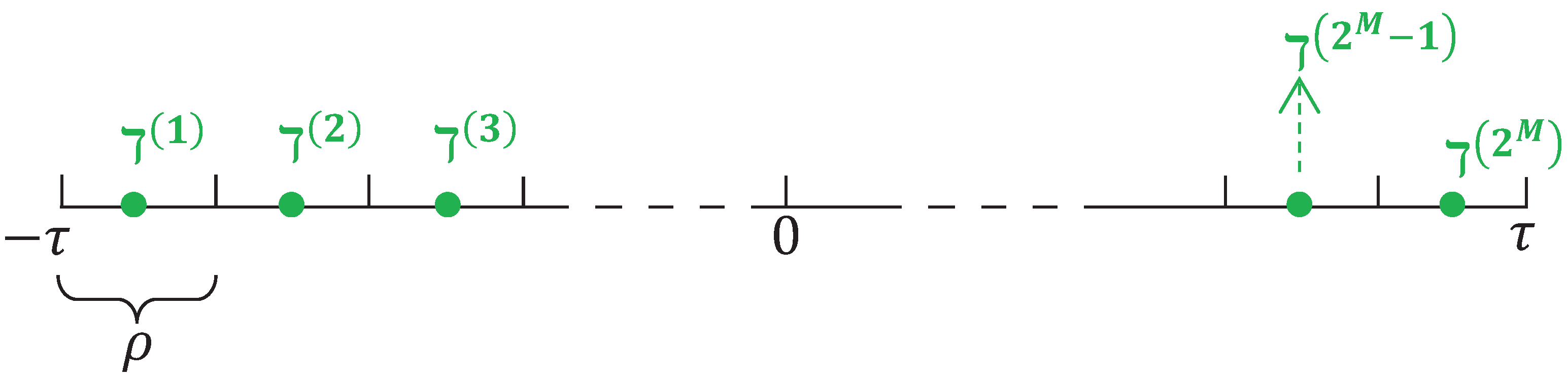
2.2. The Adoption of BESs

Considering its anti-interference features and the security of its digital communication, we chose to use the BESs during the network transmission of measurement signals $y_i\left(s\right)$ ($i=1,2,\dots ,U$) for CN (1). Suppose that the amplitude scope of a scalar signal $y_{i\iota }\left(s\right)$ ($\iota =1,2,\dots ,l_y$) at instant s is $[-\tau ,\tau ]$, where $\tau \in \mathbb{R}>0$ is a given scalar. A binary encoder was adopted to encode the measurement signal into a BBS with length M. Specifically, a uniform quantizer was utilized to quantize the output signal $y_{i\iota }\left(s\right)$ as ${\overrightarrow{y}}_{i\iota }\left(s\right)$, which corresponds to a BBS [66]. The whole measurement signal scope was divided into $2^M$ portions with a uniform interval size $\rho$, defined as follows:

$$\begin{array}{c}\hfill \rho ={\displaystyle \frac{2\tau }{2^M}}.\end{array}$$

(6)

Therefore, we obtained $2^M$ points (midpoint of every interval shown in Figure 1) defined by

$$\mathcal{O}\triangleq \{{\daleth }^{\left(1\right)},{\daleth }^{\left(2\right)},\dots ,{\daleth }^{\left(2^M\right)}\},$$

where these points are spaced uniformly and each point is expressed using the following form:

$$\begin{array}{c}\hfill {\daleth }^{\left(ϵ\right)}\triangleq -\tau +(ϵ-{\displaystyle \frac{1}{2}})\rho ,ϵ=1,2,\dots ,2^M.\end{array}$$

The quantized signals were encoded by the encoder as BBSs and transferred through the BSC, and may flip randomly; they were described by a Bernoulli-distributed random variable with a probability q owing to the presence of channel noise [66]. The decoder recovered the received BBSs at the estimator side.

Lemma 1

([66]). Define ${\xi }_{i\iota }\left(s\right)\triangleq {\overrightarrow{y}}_{i\iota }\left(s\right)-y_{i\iota }\left(s\right)$ as the quantization error. ${\xi }_{i\iota }\left(s\right)$ is an uniformly distributed stochastic variable in $[-0.5\rho ,0.5\rho ]$ satisfying

$$\begin{array}{c}\hfill \mathbb{E}\left\{{\xi }_{i\iota }\left(s\right)\right\}=0,\mathbb{V}\left\{{\xi }_{i\iota }\left(s\right)\right\}={\displaystyle \frac{{\rho }^2}{12}}\triangleq {\xi }_0^2<{\displaystyle \frac{{\rho }^2}{4}}={\displaystyle \frac{{\tau }^2}{2^{2M}}}.\end{array}$$

Lemma 2

([67]). Define ${\breve{y}}_{i\iota }\left(s\right)$ as the decoder output signal and $h_{i\iota }\left(s\right)\triangleq {\displaystyle \frac{1}{1-2q}}{\breve{y}}_{i\iota }\left(s\right)-{\overrightarrow{y}}_{i\iota }\left(s\right)$ as the equivalent noise reflecting impact from bit errors. $h_{i\iota }\left(s\right)$ has the following statistic property:

$$\begin{array}{c}\hfill \mathbb{E}\left\{h_{i\iota }\left(s\right)\right\}=0,\mathbb{V}\left\{h_{i\iota }\left(s\right)\right\}\triangleq h_0^2={\displaystyle \frac{4q(1-q)\left(2^{2M}-1\right){\tau }^2}{3{(1-2q)}^2{\left(2^M-1\right)}^2}}.\end{array}$$

In view of the aforementioned analysis, the signal used at the estimator is shown as follows:

$$\begin{array}{c}\hfill {\tilde{y}}_i\left(s\right)=y_i\left(s\right)+{\xi }_i\left(s\right)+h_i\left(s\right).\end{array}$$

(7)

Remark 1.

The uniform quantization approach, unlike probabilistic quantization (a type of random quantization), is a deterministic one that divides the scope of the signal into equally spaced quantization intervals. Typically, the midpoint of each interval is chosen as the quantized discrete value. When the length of the BBS in both [66,67] is B, the quantization error of uniform quantization in [66] seems to be reduced compared to that of probabilistic quantization in [67], and the variance bound of the quantization error in [67] is bigger (i.e., ${\displaystyle \frac{{\tau }^2}{{(2^M-1)}^2}}$) in comparison with that in [66].

Remark 2.

In (7), the description of the signal that is actually collected by the estimator is obtained via the measurement signal $y_i\left(s\right)$, the quantization error ${\xi }_i\left(s\right)$, and the equivalent noise-reflecting bit errors $h_i\left(s\right)$; this expression is beneficial to the establishment of the estimator model.

Remark 3.

The frequency of the occurrence of bit errors is measured using the bit error rate (BER), which is the percentage corresponding to the ratio of the number of flipping bits to the overall number of transferred binary bits. Here, we equate the probability of crossover to the BER. Note that bit errors may cause measurement deviations, reduce the realness and correctness of communication, and ultimately lead to a decrease in estimator performance.

2.3. The Model Establishment of Non-Fragile State Estimator

Based on the received signal ${\tilde{y}}_i\left(s\right)$ ($i=1,2,\dots ,U$) (7), a non-fragile state estimator was modelled for CN (1) as follows:

$$\begin{array}{cc}\hfill {\widehat{x}}_i(s+1)& =A_i{\widehat{x}}_i\left(s\right)+\sum _{\zeta =1}^p\sum _{j=1}^U\delta (\varkappa \left(s\right),\zeta )a_{ij}^{\left(\zeta \right)}{\mathrm{\Gamma }}^{\left(\zeta \right)}{\widehat{x}}_j\left(s\right)+B_{\mathcal{b}i}\sum _{l=1}^m{\overline{϶}}_{il}{\widehat{x}}_i(s-{\mathcal{b}}_l\left(s\right))\hfill \\ \hfill & +E_{i}g\left({\widehat{x}}_i\left(s\right)\right)+S_i\left(\varkappa \left(s\right)\right)(I_{\left(l_y\right)}+▵\left(s\right))({\tilde{y}}_i\left(s\right)-C_i{\widehat{x}}_i\left(s\right))\hfill \end{array}$$

(8)

where ${\widehat{x}}_i\left(s\right)\in {\mathbb{R}}^{l_x}$ denotes the estimate of $x_i\left(s\right)$, and $S_i\left(\varkappa \left(s\right)\right)$ ($i=1,2,\dots ,U$) describes the unknown estimator gain, which is determined later.

In (8), the gain variation is considered and represented as $▵\left(s\right)$, which has the following specific form:

$$\begin{array}{c}\hfill ▵\left(s\right)=m\mathcal{H}\left(s\right)n\end{array}$$

(9)

where $m$ and $n$ are given matrix parameters with rational dimensions, and $\mathcal{H}\left(s\right)$ is an uncertain matrix that satisfies ${\mathcal{H}}^T\left(s\right)\mathcal{H}\left(s\right)\le I_{\left(l_y\right)}$.

Setting $e_i\left(s\right)\triangleq x_i\left(s\right)-{\widehat{x}}_i\left(s\right)$ and $\overline{g}\left(e_i\left(s\right)\right)\triangleq g\left(x_i\left(s\right)\right)-g\left({\widehat{x}}_i\left(s\right)\right)$, the acquired estimation error is as follows:

$$\begin{array}{cc}\hfill e_i(s+1)=& (A_i-S_i\left(\varkappa \left(s\right)\right)(I_{\left(l_y\right)}+▵\left(s\right)C_i)e_i\left(s\right)+\sum _{\zeta =1}^p\sum _{j=1}^U\delta (\varkappa \left(s\right),\zeta )a_{ij}^{\left(\zeta \right)}{\mathrm{\Gamma }}^{\left(\zeta \right)}{e}_j\left(s\right)\hfill \\ \hfill & +B_{\mathcal{b}i}\sum _{l=1}^m{\widetilde{϶}}_{il}\left(s\right)x_i(s-{\mathcal{b}}_l\left(s\right))+B_{\mathcal{b}i}\sum _{l=1}^m{\overline{϶}}_{il}{e}_i(s-{\mathcal{b}}_l\left(s\right))+E_i\overline{g}\left(e_i\left(s\right)\right)\hfill \\ \hfill & +F_i{w}_i\left(s\right)-S_i\left(\varkappa \left(s\right)\right)(I_{\left(l_y\right)}+▵\left(s\right))D_i{v}_i\left(s\right)-S_i\left(\varkappa \left(s\right)\right)(I_{\left(l_y\right)}+▵\left(s\right)){\xi }_i\left(s\right)\hfill \\ \hfill & -S_i\left(\varkappa \left(s\right)\right)(I_{\left(l_y\right)}+▵\left(s\right))h_i\left(s\right).\hfill \end{array}$$

(10)

To simplify the expression, we present the following notations:

$$\begin{array}{cc}\hfill \mathcal{O}& \triangleq \mathrm{diag}\{{\mathcal{O}}_1,{\mathcal{O}}_2,\dots ,{\mathcal{O}}_U\}(\mathcal{O}=A,B_{\mathcal{b}},C,E,D,F),\hfill \\ \hfill S\left(\varkappa \right(s\left)\right)& \triangleq \mathrm{diag}\{S_1\left(\varkappa \left(s\right)\right),S_2\left(\varkappa \left(s\right)\right),\dots ,S_U\left(\varkappa \left(s\right)\right)\},\hfill \\ \hfill n\left(s\right)& \triangleq {[n_1^T\left(s\right)n_2^T\left(s\right)\dots n_U^T\left(s\right)]}^T(n=x,e,w,v,\xi ,h),\hfill \\ \hfill g\left(x\right(s\left)\right)& \triangleq {\left[\begin{array}{cccc}{g}^T\left(x_1\left(s\right)\right)& g^T\left(x_2\left(s\right)\right)& \cdots & g^T\left(x_U\left(s\right)\right)\end{array}\right]}^T,\hfill \\ \hfill \tilde{g}\left(e\left(s\right)\right)& \triangleq {\left[\begin{array}{cccc}{\overline{g}}^T\left(e_1\left(s\right)\right)& {\overline{g}}^T\left(e_2\left(s\right)\right)& \cdots & {\overline{g}}^T\left(e_U\left(s\right)\right)\end{array}\right]}^T,\hfill \\ \hfill {\tilde{\mathrm{\Theta }}}_l\left(s\right)& \triangleq \mathrm{diag}\{{\widetilde{϶}}_{1l}\left(s\right)I_{\left(l_x\right)},{\widetilde{϶}}_{2l}\left(s\right)I_{\left(l_x\right)},\dots ,{\widetilde{϶}}_{Ul}\left(s\right)I_{\left(l_x\right)}\},\hfill \\ \hfill {\overline{\mathrm{\Theta }}}_l& \triangleq \mathrm{diag}\{{\overline{϶}}_{1l}{I}_{\left(l_x\right)},{\overline{϶}}_{2l}{I}_{\left(l_x\right)},\dots ,{\overline{϶}}_{Ul}{I}_{\left(l_x\right)}\},\hfill \\ \hfill x(s-{\mathcal{b}}_l\left(s\right))& \triangleq {\left[\begin{array}{cccc}{x}_1^T(s-{\mathcal{b}}_l\left(s\right))& x_2^T(s-{\mathcal{b}}_l\left(s\right))& \cdots & x_U^T(s-{\mathcal{b}}_l\left(s\right))\end{array}\right]}^T,\hfill \\ \hfill e(s-{\mathcal{b}}_l\left(s\right))& \triangleq {\left[\begin{array}{cccc}{e}_1^T(s-{\mathcal{b}}_l\left(s\right))& e_2^T(s-{\mathcal{b}}_l\left(s\right))& \cdots & e_U^T(s-{\mathcal{b}}_l\left(s\right))\end{array}\right]}^T.\hfill \end{array}$$

Compact forms of (4) and (10) are attained as follows:

$$\begin{array}{cc}\hfill x(s+1)& =Ax\left(s\right)+\sum _{\zeta =1}^p\delta (\varkappa \left(s\right),\zeta ){\mathrm{\Lambda }}^{\left(\zeta \right)}\otimes {\mathrm{\Gamma }}^{\left(\zeta \right)}x\left(s\right)+\sum _{l=1}^m{\tilde{\mathrm{\Theta }}}_l\left(s\right)B_{\mathcal{b}}x(s-{\mathcal{b}}_l\left(s\right))\hfill \\ \hfill & +\sum _{l=1}^m{\overline{\mathrm{\Theta }}}_l{B}_{\mathcal{b}}x(s-{\mathcal{b}}_l\left(s\right))+Eg\left(x\left(s\right)\right)+Fw\left(s\right)\hfill \end{array}$$

(11)

and

$$\begin{array}{cc}\hfill e(s+1)& =\left(\sum _{\zeta =1}^p\delta (\varkappa \left(s\right),\zeta ){\mathrm{\Lambda }}^{\left(\zeta \right)}\otimes {\mathrm{\Gamma }}^{\left(\zeta \right)}+A-S\left(\varkappa \left(s\right)\right)I_{▵}\left(s\right)C\right)e\left(s\right)\hfill \\ \hfill & +\sum _{l=1}^m{\tilde{\mathrm{\Theta }}}_l\left(s\right)B_{\mathcal{b}}x(s-{\mathcal{b}}_l\left(s\right))+\sum _{l=1}^m{\overline{\mathrm{\Theta }}}_l{B}_{\mathcal{b}}e(s-{\mathcal{b}}_l\left(s\right))\hfill \\ \hfill & +E\tilde{g}\left(e\left(s\right)\right)+Fw\left(s\right)-S\left(\varkappa \left(s\right)\right)I_{▵}\left(s\right)Dv\left(s\right)\hfill \\ \hfill & -S\left(\varkappa \left(s\right)\right)I_{▵}\left(s\right)\xi \left(s\right)-S\left(\varkappa \left(s\right)\right)I_{▵}\left(s\right)h\left(s\right)\hfill \end{array}$$

(12)

where

$$\begin{array}{c}\hfill I_{▵}\left(s\right)\triangleq I_{\left(U{l}_y\right)}+I_{\left(U\right)}\otimes ▵\left(s\right).\end{array}$$

Let $\eta \left(s\right)\triangleq {\left[\begin{array}{cc}{x}^T\left(s\right)& e^T\left(s\right)\end{array}\right]}^T$ and $\check{g}\left(\eta \left(s\right)\right)\triangleq {\left[\begin{array}{cc}{g}^T\left(x\left(s\right)\right)& {\tilde{g}}^T\left(e\left(s\right)\right)\end{array}\right]}^T$. The following augmented SE error dynamics were derived with regard to (11)–(12):

$$\begin{array}{cc}\hfill \eta (s+1)& =\mathcal{A}\left(\varkappa \left(s\right)\right)\eta \left(s\right)+\sum _{l=1}^m{\breve{\mathbf{\Theta }}}_l\left(s\right){\mathcal{B}}_{\mathcal{b}1}\eta (s-{\mathcal{b}}_l\left(s\right))+\sum _{l=1}^m{\check{\mathbf{\Theta }}}_l{\mathcal{B}}_{\mathcal{b}2}\eta (s-{\mathcal{b}}_l\left(s\right))\hfill \\ \hfill & +\mathcal{E}\check{g}\left(\eta \left(s\right)\right)+\mathcal{F}w\left(s\right)-\mathcal{S}\left(\varkappa \left(s\right)\right)I_{▵}\left(s\right)(Dv\left(s\right)+\xi \left(s\right)+h\left(s\right))\hfill \end{array}$$

(13)

where

$$\begin{array}{cc}\hfill \mathcal{A}\left(\varkappa \right(s\left)\right)\triangleq & \mathrm{diag}\{A+\sum _{\zeta =1}^p\delta (\varkappa \left(s\right),\zeta ){\mathrm{\Lambda }}^{\left(\zeta \right)}\otimes {\mathrm{\Gamma }}^{\left(\zeta \right)},\sum _{\zeta =1}^p\delta (\varkappa \left(s\right),\zeta ){\mathrm{\Lambda }}^{\left(\zeta \right)}\otimes {\mathrm{\Gamma }}^{\left(\zeta \right)}+A-S\left(\varkappa \left(s\right)\right)\hfill \\ \hfill & \times I_{▵}\left(s\right)C\},\hfill \\ \hfill {\mathcal{B}}_{\mathcal{b}1}\triangleq & \left[\begin{array}{cc}{B}_{\mathcal{b}}& 0_{(\left(U{l}_x\right)\times \left(U{l}_x\right))}\\ B_{\mathcal{b}}& 0_{(\left(U{l}_x\right)\times \left(U{l}_x\right))}\end{array}\right],{\mathcal{B}}_{\mathcal{b}2}\triangleq \mathrm{diag}\{B_{\mathcal{b}},B_{\mathcal{b}}\},\mathcal{S}\left(\varkappa \left(s\right)\right)\triangleq \left[\begin{array}{c}{0}_{(\left(U{l}_x\right)\times \left(U{l}_y\right))}\\ S\left(\varkappa \right(s\left)\right)\end{array}\right],\hfill \\ \hfill \mathcal{E}\triangleq & \mathrm{diag}\{E,E\},{\breve{\mathbf{\Theta }}}_l\left(s\right)\triangleq \mathrm{diag}\{{\tilde{\mathrm{\Theta }}}_l\left(s\right),{\tilde{\mathrm{\Theta }}}_l\left(s\right)\},{\check{\mathbf{\Theta }}}_l\triangleq \mathrm{diag}\{{\overline{\mathrm{\Theta }}}_l,{\overline{\mathrm{\Theta }}}_l\},\mathcal{F}\triangleq {\left[\begin{array}{cc}F& F\end{array}\right]}^T.\hfill \end{array}$$

Definition 1

([5]). If there exist scalars $\varphi >0$, $0\le \psi <1$ and $m>0$ which fulfill

$$\begin{array}{c}\hfill \mathbb{E}\left\{{∥\eta \left(s\right)∥}^2\right\}\le \varphi {\psi }^s\underset{-\overline{\mathcal{b}}\le \mathsf{ȷ}\le 0}{sup}{\mathbb{E}\{\parallel \eta \left(\mathsf{ȷ}\right)\parallel }^2\}+m,\end{array}$$

(14)

then the state estimator (8) is called an exponentially ultimately bounded (EUB) estimator in the mean square for CN (1).

The goal of this paper is to design an EUB non-fragile state estimator (8) in mean square for CN (1). The SE issue discussed in this paper is shown in Figure 2.

3. Main Results

A few Lemmas are illustrated as follows; these were used for the performance analysis and estimator design (8).

Lemma 3

([68]). Considering a matrix $\mathcal{P}>0$, and vectors ${\mathcal{L}}^T$ and ${\mathcal{U}}^T$, the following inequality holds:

$$\begin{array}{c}\hfill {\mathcal{L}}^T\mathcal{P}\mathcal{U}+{\mathcal{U}}^T\mathcal{P}\mathcal{L}\le {\mathcal{L}}^T\mathcal{P}\mathcal{L}+{\mathcal{U}}^T\mathcal{P}\mathcal{U}\end{array}$$

holds.

Lemma 4

([5]). Constants $0\le f\le 1$ and γ are provided. If $\left\{J\right(s\left)\right|s=0,1,2,\dots \}$ is a nonnegative sequence with

$$\begin{array}{c}\hfill J(s+1)\le fJ\left(s\right)+\gamma ,\end{array}$$

then,

$$\begin{array}{c}\hfill J\left(s\right)\le \left\{\begin{array}{cc}J\left(0\right)+s\gamma & \mathrm{for}f=1,\\ f^{s}J\left(0\right)+{\displaystyle \frac{\gamma (1-f^s)}{1-f}}& \mathrm{for}f\ne 1.\end{array}\right.\end{array}$$

Lemma 5

([64]). Let matrices $\mathcal{X}={\mathcal{X}}^T$, $\mathcal{E}$ and $\mathcal{J}$ be of suitable sizes, and $\mathcal{F}$ meets $\mathcal{F}{\mathcal{F}}^T\le I$; then, we can obtain that $\mathcal{X}+\mathcal{J}\mathcal{F}\mathcal{E}+{\mathcal{E}}^T{\mathcal{F}}^T{\mathcal{J}}^T\le 0$ is met if and only if there is a scalar $\epsilon >0$ satisfying $\mathcal{X}+{\epsilon }^{-1}\mathcal{J}{\mathcal{J}}^T+\epsilon {\mathcal{E}}^T\mathcal{E}<0$ or

$$\begin{array}{c}\hfill \left[\begin{array}{ccc}\mathcal{X}& \ast & \ast \\ {\mathcal{J}}^T& -\epsilon I& \ast \\ \epsilon \mathcal{E}& 0& -\epsilon I\end{array}\right]<0.\end{array}$$

Now, we will analyze the estimator performance for CN (1).

Theorem 1.

Consider that the scalar $0<\kappa <1$ and the gain parameter $S_i\left(\varkappa \left(s\right)\right)$ ($i=1,2,\dots ,U$, $\varkappa \left(s\right)\in \Im$) are known. The estimator (8) becomes an EUB of CN (1) in mean square if matrices $P_a\triangleq \mathrm{diag}\{P_{1a},P_{2a}\}>0$ $(P_{1a}\triangleq \mathrm{diag}\{P_{11a},P_{12a},\dots ,P_{1Ua}\}$, $P_{2a}\triangleq \mathrm{diag}\{P_{21a},P_{22a},\dots ,P_{2Ua}\})$, $Q_v\triangleq \mathrm{diag}\{Q_{1v},Q_{2v}\}>0$ $(Q_{1v}\triangleq \mathrm{diag}\{Q_{11v},Q_{12v},$$\dots ,Q_{1Uv}\}$, $Q_{2v}\triangleq \mathrm{diag}\{Q_{21v},$$Q_{22v},\dots ,Q_{2Uv}\left\}\right)$ ($v=1,2,\dots ,m$), and scalars ${\lambda }_a>0$ satisfy the following inequality:

$$\begin{array}{c}\hfill {\mathrm{\Psi }}_a=\left[\begin{array}{ccc}{\mathrm{\Psi }}_{11a}& {\mathrm{\Psi }}_{12a}& {\mathrm{\Psi }}_{13a}\\ \ast & {\mathrm{\Psi }}_{22a}& {\mathrm{\Psi }}_{23a}\\ \ast & \ast & {\mathrm{\Psi }}_{33a}\end{array}\right]<0\end{array}$$

(15)

where

$$\begin{array}{cc}\hfill {\mathrm{\Psi }}_{11a}\triangleq & {\mathcal{A}}^T{\overline{P}}_a\mathcal{A}-{\lambda }_a{\tilde{\Xi }}_1+(1+\overline{\mathcal{b}}-\underline{\mathcal{b}})\sum _{v=1}^m{Q}_v-P_a,{\mathrm{\Psi }}_{12a}\triangleq {\mathcal{A}}^T{\overline{P}}_a(\check{\mathbf{\Theta }}\otimes {\mathcal{B}}_{\mathcal{b}2}),\hfill \\ \hfill {\overline{P}}_a\triangleq & \sum _{b=1}^p{\pi }_{ab}{P}_b,{\mathrm{\Psi }}_{13a}\triangleq {\mathcal{A}}^T{\overline{P}}_a\mathcal{E}+{\lambda }_a{\tilde{\Xi }}_2^T,{\tilde{\Xi }}_1\triangleq I_{\left(2U\right)}\otimes {\overline{\Xi }}_1,{\tilde{\Xi }}_2\triangleq I_{\left(2U\right)}\otimes {\overline{\Xi }}_2,\hfill \\ \hfill {\mathrm{\Psi }}_{22a}\triangleq & {(I_{\left(m\right)}\otimes {\mathcal{B}}_{\mathcal{b}1})}^T{\widehat{\mathrm{\Theta }}}^T(I_{\left(m\right)}\otimes {\overline{P}}_a)\widehat{\mathrm{\Theta }}(I_{\left(m\right)}\otimes {\mathcal{B}}_{\mathcal{b}1})+{(\check{\mathbf{\Theta }}\otimes {\mathcal{B}}_{\mathcal{b}2})}^T\overline{P_a}(\check{\mathbf{\Theta }}\otimes {\mathcal{B}}_{\mathcal{b}2})-{(1-\kappa )}^{\overline{\mathcal{b}}}\overline{Q},\hfill \\ \hfill {\mathrm{\Psi }}_{23a}\triangleq & {(\check{\mathbf{\Theta }}\otimes {\mathcal{B}}_{\mathcal{b}2})}^T{\overline{P}}_a\mathcal{E},{\mathrm{\Psi }}_{33a}\triangleq {\mathcal{E}}^T{\overline{P}}_a\mathcal{E}-{\lambda }_a{I}_{\left(2U{l}_x\right)},\check{\mathbf{\Theta }}\triangleq \left[\begin{array}{cccc}{\check{\mathbf{\Theta }}}_1& {\check{\mathbf{\Theta }}}_2& \cdots & {\check{\mathbf{\Theta }}}_m\end{array}\right],\hfill \\ \hfill {\overline{\Xi }}_1\triangleq & {\displaystyle \frac{{\Xi }_1^T{\Xi }_2+{\Xi }_2^T{\Xi }_1}{2}},{\overline{\Xi }}_2\triangleq {\displaystyle \frac{{\Xi }_1+{\Xi }_2}{2}},\overline{Q}\triangleq \mathrm{diag}\{Q_1,Q_2,\dots ,Q_m\},\hfill \\ \hfill {\widehat{\mathrm{\Theta }}}_l\triangleq & \mathrm{diag}\left\{\sqrt{{\overline{϶}}_{1l}(1-{\overline{϶}}_{1l})}{I}_{\left(l_x\right)},\sqrt{{\overline{϶}}_{2l}(1-{\overline{϶}}_{2l})}{I}_{\left(l_x\right)},\dots ,\sqrt{{\overline{϶}}_{Ul}(1-{\overline{϶}}_{Ul})}{I}_{\left(l_x\right)}\right\},\hfill \\ \hfill \widehat{\mathrm{\Theta }}\triangleq & \mathrm{diag}\{I_{\left(2\right)}\otimes {\widehat{\mathrm{\Theta }}}_1,I_{\left(2\right)}\otimes {\widehat{\mathrm{\Theta }}}_2,\dots ,I_{\left(2\right)}\otimes {\widehat{\mathrm{\Theta }}}_m\}.\hfill \end{array}$$

Proof of Theorem 1.

The Lyapunov functional is defined as follows:

$$\begin{array}{c}\hfill V\left(s,\eta \left(s\right),\varkappa \left(s\right)\right)\triangleq \sum _{r=1}^3{V}_r\left(s,\eta \left(s\right),\varkappa \left(s\right)\right)\end{array}$$

(16)

where

$$\begin{array}{cc}\hfill & V_1(s,\eta \left(s\right),\varkappa \left(s\right))\triangleq {\eta }^T\left(s\right)P\left(\varkappa \left(s\right)\right)\eta \left(s\right),\hfill \\ \hfill & V_2(s,\eta \left(s\right))\triangleq \sum _{v=1}^m\sum _{u=s-{\mathcal{b}}_v\left(s\right)}^{s-1}{(1-\kappa )}^{s-u-1}{\eta }^T\left(u\right)Q_v\eta \left(u\right),\hfill \\ \hfill & V_3(s,\eta \left(s\right))\triangleq \sum _{v=1}^m\sum _{n=s-\overline{\mathcal{b}}+1}^{s-\underline{\mathcal{b}}}\sum _{u=n}^{s-1}{(1-\kappa )}^{s-u-1}{\eta }^T\left(u\right)Q_v\eta \left(u\right).\hfill \end{array}$$

Letting $P_a\triangleq P\left(\varkappa \left(s\right)=a\right)$ ($a\in \Im$), and noticing that $\mathbb{E}\left\{{\breve{\mathbf{\Theta }}}_l\left(s\right)\right\}=0$, $\mathbb{E}\left\{w\right(s\left)\right\}=0$, $\mathbb{E}\left\{v\right(s\left)\right\}=0$, $\mathbb{E}\left\{\xi \right(s\left)\right\}=0$ and $\mathbb{E}\left\{h\right(s\left)\right\}=0$, one can observe from (13) that

$$\begin{array}{cc}\hfill & \mathbb{E}\left\{\mathrm{\Delta }{V}_1(s,\eta \left(s\right),\varkappa \left(s\right))\right\}=\mathbb{E}\left\{V_1\left(s+1,\eta (s+1),\varkappa (s+1)\right)|\eta \left(s\right),\varkappa \left(s\right)=a\right\}-V_1(s,\eta \left(s\right),a)\hfill \\ \hfill =& \mathbb{E}\{{\eta }^T\left(s\right){\mathcal{A}}^T{\overline{P}}_a\mathcal{A}\eta \left(s\right)-{\eta }^T\left(s\right)P_a\eta \left(s\right)+2{\eta }^T\left(s\right){\mathcal{A}}^T{\overline{P}}_a\mathcal{E}\check{g}\left(\eta \left(s\right)\right)+2{\eta }^T\left(s\right){\mathcal{A}}^T{\overline{P}}_a(\check{\mathbf{\Theta }}\otimes {\mathcal{B}}_{\mathcal{b}2})\hfill \\ \hfill & \times \eta (s-\mathcal{b}\left(s\right))+{\check{g}}^T\left(\eta \left(s\right)\right){\mathcal{E}}^T{\overline{P}}_a\mathcal{E}\check{g}\left(\eta \left(s\right)\right)+w^T\left(s\right){\mathcal{F}}^T{\overline{P}}_a\mathcal{F}w\left(s\right)+{\eta }^T(s-\mathcal{b}\left(s\right)){(I_{\left(m\right)}\otimes {\mathcal{B}}_{\mathcal{b}1})}^T\hfill \\ \hfill & \times {\widehat{\mathrm{\Theta }}}^T(I_{\left(m\right)}\otimes {\overline{P}}_a)\widehat{\mathrm{\Theta }}(I_{\left(m\right)}\otimes {\mathcal{B}}_{\mathcal{b}1})\eta (s-\mathcal{b}\left(s\right))+{\eta }^T(s-\mathcal{b}\left(s\right)){(\check{\mathbf{\Theta }}\otimes {\mathcal{B}}_{\mathcal{b}2})}^T{\overline{P}}_a(\check{\mathbf{\Theta }}\otimes {\mathcal{B}}_{\mathcal{b}2})\hfill \\ \hfill & \times \eta (s-\mathcal{b}\left(s\right))+2{\eta }^T(s-\mathcal{b}\left(s\right)){(\check{\mathbf{\Theta }}\otimes {\mathcal{B}}_{\mathcal{b}2})}^T{\overline{P}}_a\mathcal{E}\check{g}\left(\eta \left(s\right)\right)+v^T\left(s\right)D^T{I}_{▵}^T\left(s\right){\mathcal{S}}_a^T{\overline{P}}_a{\mathcal{S}}_a{I}_{▵}\left(s\right)\hfill \\ \hfill & \times Dv\left(s\right)+{\xi }^T\left(s\right)I_{▵}^T\left(s\right){\mathcal{S}}_a^T{\overline{P}}_a{\mathcal{S}}_a{I}_{▵}\left(s\right)\xi \left(s\right)+h^T\left(s\right)I_{▵}^T\left(s\right){\mathcal{S}}_a^T{\overline{P}}_a{\mathcal{S}}_a{I}_{▵}\left(s\right)h\left(s\right)\hfill \\ \hfill & +2v^T\left(s\right)D^T{I}_{▵}^T\left(s\right){\mathcal{S}}_a^T{\overline{P}}_a{\mathcal{S}}_a{I}_{▵}\left(s\right)\xi \left(s\right)+2v^T\left(s\right)D^T{I}_{▵}^T\left(s\right){\mathcal{S}}_a^T{\overline{P}}_a{\mathcal{S}}_a{I}_{▵}\left(s\right)h\left(s\right)\hfill \\ \hfill & +2{\xi }^T\left(s\right)I_{▵}^T\left(s\right){\mathcal{S}}_a^T{\overline{P}}_a{\mathcal{S}}_a{I}_{▵}\left(s\right)h\left(s\right)\}.\hfill \end{array}$$

Using Lemma 3, we can obtain the following inequalities:

$$\begin{array}{cc}\hfill & 2v^T\left(s\right)D^T{I}_{▵}^T\left(s\right){\mathcal{S}}_a^T{\overline{P}}_a{\mathcal{S}}_a{I}_{▵}\left(s\right)\xi \left(s\right)\hfill \end{array}$$

$$\begin{array}{cc}\hfill \le & v^T\left(s\right)D^T{I}_{▵}^T\left(s\right){\mathcal{S}}_a^T{\overline{P}}_a{\mathcal{S}}_a{I}_{▵}\left(s\right)Dv\left(s\right)+{\xi }^T\left(s\right)I_{▵}^T\left(s\right){\mathcal{S}}_a^T{\overline{P}}_a{\mathcal{S}}_a{I}_{▵}\left(s\right)\xi \left(s\right),\hfill \\ \hfill & 2v^T\left(s\right)D^T{I}_{▵}^T\left(s\right){\mathcal{S}}_a^T{\overline{P}}_a{\mathcal{S}}_a{I}_{▵}\left(s\right)h\left(s\right)\hfill \end{array}$$

(17)

$$\begin{array}{cc}\hfill \le & v^T\left(s\right)D^T{I}_{▵}^T\left(s\right){\mathcal{S}}_a^T{\overline{P}}_a{\mathcal{S}}_a{I}_{▵}\left(s\right)Dv\left(s\right)+h^T\left(s\right)I_{▵}^T\left(s\right){\mathcal{S}}_a^T{\overline{P}}_a{\mathcal{S}}_a{I}_{▵}\left(s\right)h\left(s\right),\hfill \\ \hfill & 2{\xi }^T\left(s\right)I_{▵}^T\left(s\right){\mathcal{S}}_a^T{\overline{P}}_a{\mathcal{S}}_a{I}_{▵}\left(s\right)h\left(s\right)\hfill \end{array}$$

(18)

$$\begin{array}{cc}\hfill \le & {\xi }^T\left(s\right)I_{▵}^T\left(s\right){\mathcal{S}}_a^T{\overline{P}}_a{\mathcal{S}}_a{I}_{▵}\left(s\right)\xi \left(s\right)+h^T\left(s\right)I_{▵}^T\left(s\right){\mathcal{S}}_a^T{\overline{P}}_a{\mathcal{S}}_a{I}_{▵}\left(s\right)h\left(s\right)\hfill \end{array}$$

(19)

By utilizing the property $\mathsf{F}\beth =\beth \mathsf{F}$ (where $\mathsf{F}$ and ℶ are two diagonal matrices), and the characteristic of matrix trace ($\mathrm{tr}\left\{WY\right\}=\mathrm{tr}\left\{YW\right\}$, $\mathrm{tr}\left\{c\right\}=c$ (where $c\in \mathbb{R}$ is a constant) and $\mathrm{tr}\left\{\mathrm{diag}\right\{W,Y\left\}\right\}=\mathrm{tr}\left\{W\right\}+\mathrm{tr}\left\{Y\right\}$), and combining this with (17)–(19), we obtain the following:

$$\begin{array}{cc}\hfill & \mathbb{E}\left\{\mathrm{\Delta }{V}_1(s,\eta \left(s\right),\varkappa \left(s\right))\right\}\hfill \\ \hfill \le & \mathbb{E}\{{\eta }^T\left(s\right){\mathcal{A}}^T{\overline{P}}_a\mathcal{A}\eta \left(s\right)-{\eta }^T\left(s\right)P_a\eta \left(s\right)+2{\eta }^T\left(s\right){\mathcal{A}}^T{\overline{P}}_a\mathcal{E}\check{g}\left(\eta \left(s\right)\right)+2{\eta }^T\left(s\right){\mathcal{A}}^T{\overline{P}}_a(\check{\mathbf{\Theta }}\otimes {\mathcal{B}}_{\mathcal{b}2})\hfill \\ \hfill & \times \eta (s-\mathcal{b}\left(s\right))+{\check{g}}^T\left(\eta \left(s\right)\right){\mathcal{E}}^T{\overline{P}}_a\mathcal{E}\check{g}\left(\eta \left(s\right)\right)+{\eta }^T(s-\mathcal{b}\left(s\right)){(I_{\left(m\right)}\otimes {\mathcal{B}}_{\mathcal{b}1})}^T{\widehat{\mathrm{\Theta }}}^T(I_{\left(m\right)}\otimes {\overline{P}}_a)\widehat{\mathrm{\Theta }}\hfill \\ \hfill & \times (I_{\left(m\right)}\otimes {\mathcal{B}}_{\mathcal{b}1})\eta (s-\mathcal{b}\left(s\right))+{\eta }^T(s-\mathcal{b}\left(s\right)){(\check{\mathbf{\Theta }}\otimes {\mathcal{B}}_{\mathcal{b}2})}^T{\overline{P}}_a(\check{\mathbf{\Theta }}\otimes {\mathcal{B}}_{\mathcal{b}2})\eta (s-\mathcal{b}\left(s\right))\hfill \\ \hfill & +2{\eta }^T(s-\mathcal{b}\left(s\right)){(\check{\mathbf{\Theta }}\otimes {\mathcal{B}}_{\mathcal{b}2})}^T{\overline{P}}_a\mathcal{E}\check{g}\left(\eta \left(s\right)\right)\hfill \\ \hfill & +\mathrm{tr}\left\{{\mathcal{F}}^T{\overline{P}}_a\mathcal{F}w\left(s\right)w^T\left(s\right)\right\}+\mathrm{tr}\left\{3D^T{I}_{▵}^T\left(s\right){\mathcal{S}}_a^T{\overline{P}}_a{\mathcal{S}}_a{I}_{▵}\left(s\right)Dv\left(s\right)v^T\left(s\right)\right\}\hfill \\ \hfill & +\mathrm{tr}\{3I_{▵}^T\left(s\right){\mathcal{S}}_a^T{\overline{P}}_a{\mathcal{S}}_a{I}_{▵}\left(s\right)\xi \left(s\right){\xi }^T\left(s\right)+3I_{▵}^T\left(s\right){\mathcal{S}}_a^T{\overline{P}}_a{\mathcal{S}}_a{I}_{▵}\left(s\right)h\left(s\right)h^T\left(s\right)\}\}\hfill \end{array}$$

(20)

where

$$\begin{array}{cc}\hfill & \eta (s-\mathcal{b}\left(s\right))\triangleq {\left[\begin{array}{cccc}{\eta }^T(s-{\mathcal{b}}_1\left(s\right))& {\eta }^T(s-{\mathcal{b}}_2\left(s\right))& \cdots & {\eta }^T(s-{\mathcal{b}}_m\left(s\right))\end{array}\right]}^T,\hfill \end{array}$$

$$\begin{array}{cc}\hfill & \mathbb{E}\left\{\mathrm{\Delta }{V}_2(s,\eta \left(s\right))\right\}\hfill \\ \hfill =& \mathbb{E}\left\{\sum _{v=1}^m\sum _{u=s-{\mathcal{b}}_v(s+1)+1}^s{(1-\kappa )}^{s-u}{\eta }^T\left(u\right)Q_v\eta \left(u\right)-\sum _{v=1}^m\sum _{u=s-{\mathcal{b}}_v\left(s\right)}^{s-1}{(1-\kappa )}^{s-u-1}{\eta }^T\left(u\right)Q_v\eta \left(u\right)\right\}\hfill \\ \hfill =& \sum _{v=1}^m\{{\eta }^T\left(s\right)Q_v\eta \left(s\right)+\sum _{u=s-{\mathcal{b}}_v(s+1)+1}^{s-1}{(1-\kappa )}^{s-u}{\eta }^T\left(u\right)Q_v\eta \left(u\right)\hfill \\ \hfill & -\sum _{u=s-{\mathcal{b}}_v\left(s\right)}^{s-1}{(1-\kappa )}^{s-u-1}{\eta }^T\left(u\right)Q_v\eta \left(u\right)\}\hfill \\ \hfill \le & \sum _{v=1}^m\{{\eta }^T\left(s\right)Q_v\eta \left(s\right)+\sum _{u=s-\overline{\mathcal{b}}+1}^{s-\underline{\mathcal{b}}}{(1-\kappa )}^{s-u}{\eta }^T\left(u\right)Q_v\eta \left(u\right)+\sum _{u=s-{\mathcal{b}}_v\left(s\right)+1}^{s-1}{(1-\kappa )}^{s-u}{\eta }^T\left(u\right)\hfill \\ \hfill & \times Q_v\eta \left(u\right)-\sum _{u=s-{\mathcal{b}}_v\left(s\right)}^{s-1}{(1-\kappa )}^{s-u-1}{\eta }^T\left(u\right)Q_v\eta \left(u\right)\}\hfill \\ \hfill =& \sum _{v=1}^m\{{\eta }^T\left(s\right)Q_v\eta \left(s\right)+\sum _{u=s-\overline{\mathcal{b}}+1}^{s-\underline{\mathcal{b}}}{(1-\kappa )}^{s-u}{\eta }^T\left(u\right)Q_v\eta \left(u\right)+\sum _{u=s-{\mathcal{b}}_v\left(s\right)}^{s-1}{(1-\kappa )}^{s-u}{\eta }^T\left(u\right)Q_v\hfill \\ \hfill & \times \eta \left(u\right)-{(1-\kappa )}^{{\mathcal{b}}_v\left(s\right)}{\eta }^T(s-{\mathcal{b}}_v\left(s\right))Q_v\eta (s-{\mathcal{b}}_v\left(s\right))-\sum _{u=s-{\mathcal{b}}_v\left(s\right)}^{s-1}{(1-\kappa )}^{s-u-1}{\eta }^T\left(u\right)Q_v\eta \left(u\right)\}\hfill \\ \hfill \le & \sum _{v=1}^m\{{\eta }^T\left(s\right)Q_v\eta \left(s\right)+\sum _{u=s-\overline{\mathcal{b}}+1}^{s-\underline{\mathcal{b}}}{(1-\kappa )}^{s-u}{\eta }^T\left(u\right)Q_v\eta \left(u\right)-{(1-\kappa )}^{\overline{\mathcal{b}}}{\eta }^T(s-{\mathcal{b}}_v\left(s\right))Q_v\hfill \\ \hfill & \times \eta (s-{\mathcal{b}}_v\left(s\right))-\kappa \sum _{u=s-{\mathcal{b}}_v\left(s\right)}^{s-1}{(1-\kappa )}^{s-u-1}{\eta }^T\left(u\right)Q_v\eta \left(u\right)\}\hfill \\ \hfill =& \sum _{v=1}^m\{{\eta }^T\left(s\right)Q_v\eta \left(s\right)+\sum _{u=s-\overline{\mathcal{b}}+1}^{s-\underline{\mathcal{b}}}{(1-\kappa )}^{s-u}{\eta }^T\left(u\right)Q_v\eta \left(u\right)-{(1-\kappa )}^{\overline{\mathcal{b}}}{\eta }^T(s-{\mathcal{b}}_v\left(s\right))Q_v\hfill \\ \hfill & \times \eta (s-{\mathcal{b}}_v\left(s\right))\}-\kappa V_2(s,\eta \left(s\right))\hfill \end{array}$$

(21)

and

$$\begin{array}{cc}\hfill & \mathbb{E}\left\{\mathrm{\Delta }{V}_3(s,\eta \left(s\right))\right\}\hfill \\ \hfill =& \mathbb{E}\{\sum _{v=1}^m\sum _{n=s-\overline{\mathcal{b}}+2}^{s+1-\underline{\mathcal{b}}}\sum _{u=n}^s{(1-\kappa )}^{s-u}{\eta }^T\left(u\right)Q_v\eta \left(u\right)-\sum _{v=1}^m\sum _{n=s-\overline{\mathcal{b}}+1}^{s-\underline{\mathcal{b}}}\sum _{u=n}^{s-1}{(1-\kappa )}^{s-u-1}\hfill \\ \hfill & \times {\eta }^T\left(u\right)Q_v\eta \left(u\right)\}\hfill \\ \hfill =& \sum _{v=1}^m\{(\overline{\mathcal{b}}-\underline{\mathcal{b}}){\eta }^T\left(s\right)Q_v\eta \left(s\right)+\sum _{n=s-\overline{\mathcal{b}}+2}^{s+1-\underline{\mathcal{b}}}\sum _{u=n}^{s-1}{(1-\kappa )}^{s-u}{\eta }^T\left(u\right)Q_v\eta \left(u\right)\hfill \\ \hfill & -\sum _{n=s-\overline{\mathcal{b}}+1}^{s-\underline{\mathcal{b}}}\sum _{u=n}^{s-1}{(1-\kappa )}^{s-u-1}{\eta }^T\left(u\right)Q_v\eta \left(u\right)\}\hfill \\ \hfill =& \sum _{v=1}^m\{(\overline{\mathcal{b}}-\underline{\mathcal{b}}){\eta }^T\left(s\right)Q_v\eta \left(s\right)+\sum _{n=s-\overline{\mathcal{b}}+1}^{s-\underline{\mathcal{b}}}\sum _{u=n+1}^{s-1}{(1-\kappa )}^{s-u}{\eta }^T\left(u\right)Q_v\eta \left(u\right)\hfill \\ \hfill & -\sum _{n=s-\overline{\mathcal{b}}+1}^{s-\underline{\mathcal{b}}}\sum _{u=n}^{s-1}{(1-\kappa )}^{s-u-1}{\eta }^T\left(u\right)Q_v\eta \left(u\right)\}\hfill \\ \hfill =& \sum _{v=1}^m\{(\overline{\mathcal{b}}-\underline{\mathcal{b}}){\eta }^T\left(s\right)Q_v\eta \left(s\right)-\sum _{u=s-\overline{\mathcal{b}}+1}^{s-\underline{\mathcal{b}}}{(1-\kappa )}^{s-u}{\eta }^T\left(u\right)Q_v\eta \left(u\right)+\sum _{n=s-\overline{\mathcal{b}}+1}^{s-\underline{\mathcal{b}}}\sum _{u=n}^{s-1}{(1-\kappa )}^{s-u}\hfill \\ \hfill & \times {\eta }^T\left(u\right)Q_v\eta \left(u\right)-\sum _{n=s-\overline{\mathcal{b}}+1}^{s-\underline{\mathcal{b}}}\sum _{u=n}^{s-1}{(1-\kappa )}^{s-u-1}{\eta }^T\left(u\right)Q_v\eta \left(u\right)\}\hfill \\ \hfill =& \sum _{v=1}^m\{(\overline{\mathcal{b}}-\underline{\mathcal{b}}){\eta }^T\left(s\right)Q_v\eta \left(s\right)-\sum _{u=s-\overline{\mathcal{b}}+1}^{s-\underline{\mathcal{b}}}{(1-\kappa )}^{s-u}{\eta }^T\left(u\right)Q_v\eta \left(u\right)\hfill \\ \hfill & -\kappa \sum _{n=s-\overline{\mathcal{b}}+1}^{s-\underline{\mathcal{b}}}\sum _{u=n}^{s-1}{(1-\kappa )}^{s-u-1}{\eta }^T\left(u\right)Q_v\eta \left(u\right)\}\hfill \\ \hfill =& \sum _{v=1}^m\left\{(\overline{\mathcal{b}}-\underline{\mathcal{b}}){\eta }^T\left(s\right)Q_v\eta \left(s\right)-\sum _{u=s-\overline{\mathcal{b}}+1}^{s-\underline{\mathcal{b}}}{(1-\kappa )}^{s-u}{\eta }^T\left(u\right)Q_v\eta \left(u\right)\right\}-\kappa V_3(s,\eta \left(s\right)).\hfill \end{array}$$

(22)

Based on (3), we know that

$$\begin{array}{c}\hfill {\left[\begin{array}{c}{x}_i\left(s\right)\\ g\left(x_i\left(s\right)\right)\end{array}\right]}^T\left[\begin{array}{cc}{\overline{\Xi }}_1& -{\overline{\Xi }}_2^T\\ \ast & I_{\left(l_x\right)}\end{array}\right]\left[\begin{array}{c}{x}_i\left(s\right)\\ g\left(x_i\left(s\right)\right)\end{array}\right]\le 0,\end{array}$$

(23)

$$\begin{array}{c}\hfill {\left[\begin{array}{c}{e}_i\left(s\right)\\ \overline{g}\left(e_i\left(s\right)\right)\end{array}\right]}^T\left[\begin{array}{cc}{\overline{\Xi }}_1& -{\overline{\Xi }}_2^T\\ \ast & I_{\left(l_x\right)}\end{array}\right]\left[\begin{array}{c}{e}_i\left(s\right)\\ \overline{g}\left(e_i\left(s\right)\right)\end{array}\right]\le 0.\end{array}$$

(24)

The compact forms of (23) and (24) can be acquired as follows:

$$\begin{array}{c}\hfill {\left[\begin{array}{c}\eta \left(s\right)\\ \check{g}\left(\eta \left(s\right)\right)\end{array}\right]}^T\left[\begin{array}{cc}{\tilde{\Xi }}_1& -{\tilde{\Xi }}_2^T\\ \ast & I_{\left(2U{l}_x\right)}\end{array}\right]\left[\begin{array}{c}\eta \left(s\right)\\ \check{g}\left(\eta \left(s\right)\right)\end{array}\right]\le 0.\end{array}$$

(25)

To summarize the above discussions, the following inequality is obtained:

$$\begin{array}{cc}\hfill & \mathbb{E}\left\{\mathrm{\Delta }V(s,\eta (s),a)\right\}\le {\zeta }^T\left(s\right){\mathrm{\Psi }}_a\zeta \left(s\right)-\kappa V(s,\eta \left(s\right),a)+\mathrm{tr}\left\{{\mathrm{\Phi }}_a\right\}\hfill \end{array}$$

(26)

where

$$\begin{array}{cc}\hfill \zeta \left(s\right)\triangleq & {\left[\begin{array}{ccc}{\eta }^T\left(s\right)& {\eta }^T(s-\mathcal{b}\left(s\right))& {\check{g}}^T\left(\eta \left(s\right)\right)\end{array}\right]}^T,\hfill \\ \hfill {\mathrm{\Phi }}_a\triangleq & \mathrm{diag}\{w_0^2{\mathcal{F}}^T{\overline{P}}_a\mathcal{F},3v_0^2{D}^T{I}_{▵}^T\left(s\right){\mathcal{S}}_a^T{\overline{P}}_a{\mathcal{S}}_a{I}_{▵}\left(s\right)D,3{\xi }_0^2{I}_{▵}^T\left(s\right){\mathcal{S}}_a^T{\overline{P}}_a{\mathcal{S}}_a{I}_{▵}\left(s\right)\hfill \\ \hfill & +3h_0^2{I}_{▵}^T\left(s\right){\mathcal{S}}_a^T{\overline{P}}_a{\mathcal{S}}_a{I}_{▵}\left(s\right)\}.\hfill \end{array}$$

Considering (15), we can obtain from (26) that

$$\begin{array}{c}\hfill \mathbb{E}\left\{V(s+1,\eta (s+1),\varkappa (s+1\left)\right)\left|\eta \right(s),\varkappa (s)=a\right\}\le (1-\kappa )\mathbb{E}\left\{V(s,\eta \left(s\right),a)\right\}+\mathrm{tr}\left({\mathrm{\Phi }}_a\right).\end{array}$$

(27)

By utilizing Lemma 4, the following is obtained:

$$\begin{array}{cc}\hfill & \mathbb{E}\left\{V(s,\eta (s),a)\right\}\le {(1-\kappa )}^s\mathbb{E}\left\{V(0,\eta \left(0\right),a)\right\}+{\displaystyle \frac{(1-{(1-\kappa )}^s)\mathrm{tr}\left({\mathrm{\Phi }}_a\right)}{\kappa }}.\hfill \end{array}$$

(28)

Using (16), it can be observed that

$$\begin{array}{c}\hfill \mathbb{E}\left\{V(s,\eta (s),a)\right\}\ge {\phi }_{min}\left(P_a\right)\mathbb{E}\left\{{\parallel \eta \left(s\right)\parallel }^2\right\}\end{array}$$

(29)

and

$$\begin{array}{c}\hfill \mathbb{E}\left\{V(0,\eta (0),a)\right\}\le \overline{\varphi }\underset{-\overline{\mathcal{b}}\le \mathsf{ȷ}\le 0}{sup}{\mathbb{E}\{\parallel \eta \left(\mathsf{ȷ}\right)\parallel }^2\}\end{array}$$

(30)

where

$$\begin{array}{c}\hfill \overline{\varphi }\triangleq {\phi }_{max}\left(P_a\right)+({\overline{\mathcal{b}}}^2-\overline{\mathcal{b}}\underline{\mathcal{b}}+\underline{\mathcal{b}})\sum _{v=1}^m{\phi }_{max}\left(Q_v\right)\end{array}$$

Accordingly, an inequality is obtained from (28)–(30) as follows:

$$\begin{array}{cc}\hfill \mathbb{E}\left\{{\parallel \eta \left(s\right)\parallel }^2\right\}\le & {\displaystyle \frac{{(1-\kappa )}^s\mathbb{E}\left\{V(0,\eta (0),a)\right\}}{{\phi }_{min}\left(P_a\right)}}+{\displaystyle \frac{\mathrm{tr}\left(\mathrm{\Phi }\right)}{\kappa {\phi }_{min}\left(P_a\right)}}\hfill \\ \hfill \le & {\displaystyle \frac{\overline{\varphi }}{{\phi }_{min}\left(P_a\right)}}{(1-\kappa )}^s\underset{-\overline{\mathcal{b}}\le \mathsf{ȷ}\le 0}{sup}{\mathbb{E}\{\parallel \eta \left(\mathsf{ȷ}\right)\parallel }^2\}+{\displaystyle \frac{\mathrm{tr}\left(\mathrm{\Phi }\right)}{\kappa {\phi }_{min}\left(P_a\right)}}.\hfill \end{array}$$

In terms of Definition 1, it can be observed that the dynamics of the estimation error are EUB in mean square, and the ultimate error bound is shown as follows:

$$\begin{array}{c}\hfill {\displaystyle \frac{\mathrm{tr}\left(\mathrm{\Phi }\right)}{\kappa {\phi }_{min}\left(P_a\right)}}.\end{array}$$

The SE error can be expressed using $e\left(s\right)\triangleq W\eta \left(s\right)$ with $W\triangleq \left[\begin{array}{cc}{0}_{(\left(U{l}_x\right)\times \left(U{l}_x\right))}& I_{\left(U{l}_x\right)}\end{array}\right]$. In the upcoming section, we aimed to design a gain parameter for a non-fragile estimator (8). □

Theorem 2.

Consider that scalar $0<\kappa <1$ is known. The constructed estimator (8) becomes an EUB state estimator of CN (1) in mean square as long as matrices $P_a\triangleq \mathrm{diag}\{P_{1a},P_{2a}\}>0$ $(P_{1a}\triangleq \mathrm{diag}\{P_{11a},P_{12a},\dots ,P_{1Ua}\}$, $P_{2a}\triangleq \mathrm{diag}\{P_{21a},P_{22a},\dots ,P_{2Ua}\})$, $Q_v\triangleq \mathrm{diag}\{Q_{1v},Q_{2v}\}>0$ $(Q_{1v}\triangleq \mathrm{diag}\{Q_{11v},Q_{12v},\dots ,Q_{1Uv}\}$, $Q_{2v}\triangleq \mathrm{diag}\{Q_{21v},Q_{22v},\dots ,$$Q_{2Uv}\}$, $v=1,\dots ,m)$, $\mathcal{R}>0$ ($\mathcal{R}=\mathrm{diag}\{{\mathcal{R}}_1,{\mathcal{R}}_2,{\mathcal{R}}_3\}$), a matrix $G_a\triangleq {\left[\begin{array}{cc}{0}_{(\left(U{l}_y\right)\times \left(U{l}_x\right))}& G_{2a}^T\end{array}\right]}^T$$(G_{2a}\triangleq \mathrm{diag}\{G_{21a},G_{22a},\dots ,$$G_{2Ua}\left\}\right)$, and scalars ${\lambda }_a>0$, ${\epsilon }_a>0$, and ${\varrho }_a>0$ satisfy the following linear matrix inequalities:

$$\begin{array}{c}\hfill \left[\begin{array}{ccccccc}{{\rm Y}}_{11a}& \ast & \ast & \ast & \ast & \ast & \ast \\ 0& {{\rm Y}}_{22}& \ast & \ast & \ast & \ast & \ast \\ {{\rm Y}}_{31a}& 0& {{\rm Y}}_{33a}& \ast & \ast & \ast & \ast \\ {{\rm Y}}_{41a}& {{\rm Y}}_{42a}& {\overline{P}}_a\mathcal{E}& -{\overline{P}}_a& 0& \ast & \ast \\ 0& {{\rm Y}}_{52a}& 0& 0& -I_{\left(m\right)}\otimes {\overline{P}}_a& \ast & \ast \\ 0& 0& 0& {{\rm Y}}_{64a}& 0& -{\epsilon }_a{I}_{\left(2U{l}_y\right)}& \ast \\ {{\rm Y}}_{71a}& 0& 0& 0& 0& 0& -{\epsilon }_a{I}_{\left(2U{l}_y\right)}\end{array}\right]<0,\end{array}$$

(31)

$$\begin{array}{c}\hfill \left[\begin{array}{cccc}-\mathcal{R}& \ast & \ast & \ast \\ {\mathcal{K}}_a& -I_{\left(4\right)}\otimes {\overline{P}}_a& \ast & \ast \\ 0& {\widehat{m}}_a^T& -{\varrho }_a{I}_{\left(2U{l}_y\right)}& \ast \\ {\varrho }_a\widehat{n}& 0& 0& -{\varrho }_a{I}_{\left(2U{l}_y\right)}\end{array}\right]<0,\end{array}$$

(32)

$$\begin{array}{c}\hfill W^{T}W<P_a\end{array}$$

(33)

where

$$\begin{array}{cc}\hfill {{\rm Y}}_{11a}& \triangleq -{\lambda }_a{\tilde{\Xi }}_1+(1+\overline{\mathcal{b}}-\underline{\mathcal{b}})\sum _{v=1}^m{Q}_v-P_a,{{\rm Y}}_{22}\triangleq -{(1-\kappa )}^{\overline{\mathcal{b}}}\overline{Q},\hfill \\ \hfill {{\rm Y}}_{33a}& \triangleq -{\lambda }_a{I}_{\left(2U{l}_x\right)},{{\rm Y}}_{41a}\triangleq {\overline{P}}_a{\overline{\mathcal{A}}}_a+G_a{\overline{\mathcal{C}}}_1,{{\rm Y}}_{42a}\triangleq {\overline{P}}_a(\check{\mathbf{\Theta }}\otimes {\mathcal{B}}_{\mathcal{b}2}),\hfill \\ \hfill {{\rm Y}}_{52a}& \triangleq (I_{\left(m\right)}\otimes {\overline{P}}_a)\widehat{\mathrm{\Theta }}(I_{\left(m\right)}\otimes {\mathcal{B}}_{\mathcal{b}1}),{{\rm Y}}_{31a}\triangleq {\lambda }_a{\tilde{\Xi }}_2,{{\rm Y}}_{64a}\triangleq -{\overline{m}}^T{G}_a^T,\hfill \\ \hfill {{\rm Y}}_{71a}& \triangleq \mathrm{diag}\{0_{(\left(U{l}_y\right)\times \left(U{l}_x\right))},{\epsilon }_a(I_{\left(U\right)}\otimes n)C\},{\overline{\mathcal{C}}}_1\triangleq \left[\begin{array}{cc}{0}_{(\left(U{l}_y\right)\times \left(U{l}_x\right))}& -C\end{array}\right],\hfill \\ \hfill {\overline{\mathcal{A}}}_a& \triangleq \mathrm{diag}\left\{A+{\mathrm{\Lambda }}^{\left(a\right)}\otimes {\mathrm{\Gamma }}^{\left(a\right)},A+{\mathrm{\Lambda }}^{\left(a\right)}\otimes {\mathrm{\Gamma }}^{\left(a\right)}\right\},\overline{m}\triangleq \left[\begin{array}{cc}{0}_{(\left(U{l}_y\right)\times \left(U{l}_y\right))}& I_{\left(U\right)}\otimes m\end{array}\right],\hfill \\ \hfill {\mathcal{K}}_a& \triangleq \left[\begin{array}{ccc}{w}_0{\overline{P}}_a\mathcal{F}& 0& 0\\ 0& \sqrt{3}{v}_0{G}_{a}D& 0\\ 0& 0& \sqrt{3}{\xi }_0{G}_a\\ 0& 0& \sqrt{3}{h}_0{G}_a\end{array}\right],\widehat{n}\triangleq \left[\begin{array}{ccc}0& (I_{\left(U\right)}\otimes n)D& 0\\ 0& 0& I_{\left(U\right)}\otimes n\end{array}\right],\hfill \\ \hfill {\widehat{m}}_a& \triangleq \left[\begin{array}{cc}0& 0\\ \sqrt{3}{v}_0{G}_a(I_{\left(U\right)}\otimes m)& 0\\ 0& \sqrt{3}{\xi }_0{G}_a(I_{\left(U\right)}\otimes m)\\ 0& \sqrt{3}{h}_0{G}_a(I_{\left(U\right)}\otimes m)\end{array}\right].\hfill \end{array}$$

Additionally, the minimum ultimate bound of estimation error $\mathbb{E}\left\{{∥e\left(s\right)∥}^2\right\}$ is attained via settling the following optimization issue:

$$\begin{array}{c}\hfill \underset{\mathit{subject} \mathit{to} \mathit{\left(}\mathsf{31}\mathit{\right)}–\mathit{\left(}\mathsf{33}\mathit{\right)}}{min}\mathrm{tr}\left(\mathcal{R}\right).\end{array}$$

(34)

The gain expression for the state estimator (8) is presented as follows:

$$\begin{array}{c}\hfill S_{ia}\triangleq {\overline{P}}_{2ia}^{-1}{G}_{2ia}.\end{array}$$

(35)

Proof of Theorem 2.

Defining ${\overline{P}}_a{\mathcal{S}}_a\triangleq G_a$ and ${\overline{P}}_{2ia}{S}_{ia}\triangleq G_{2ia}$, through the application of Schur Complement Lemma and Lemma 5, (15) holds as long as (31) holds.

Considering ${\mathrm{\Phi }}_a={\widehat{\mathcal{K}}}_a^T{(I_{\left(4\right)}\otimes {\overline{P}}_a)}^{-1}{\widehat{\mathcal{K}}}_a$ with

$$\begin{array}{cc}\hfill {\widehat{\mathcal{K}}}_a& \triangleq \left[\begin{array}{ccc}{w}_0{\overline{P}}_a\mathcal{F}& 0& 0\\ 0& \sqrt{3}{v}_0{\overline{P}}_a{\mathcal{S}}_a{I}_{▵}\left(s\right)D& 0\\ 0& 0& \sqrt{3}{\xi }_0{\overline{P}}_a{\mathcal{S}}_a{I}_{▵}\left(s\right)\\ 0& 0& \sqrt{3}{h}_0{\overline{P}}_a{\mathcal{S}}_a{I}_{▵}\left(s\right)\end{array}\right],\hfill \end{array}$$

we can obtain from (32) that

$$\begin{array}{c}\hfill {\mathrm{\Phi }}_a<\mathcal{R}.\end{array}$$

(36)

By combining (28) with (36), we can derive the following:

$$\begin{array}{cc}\hfill \mathbb{E}\left\{V(s,\eta (s),a)\right\}& <{(1-\kappa )}^s\mathbb{E}\left\{V(0,\eta \left(0\right),a)\right\} + {\displaystyle \frac{\mathrm{tr}\left({\mathrm{\Phi }}_a\right)}{\kappa }}\hfill \\ \hfill & <{(1-\kappa )}^s\mathbb{E}\left\{V(0,\eta \left(0\right),a)\right\} + {\displaystyle \frac{\mathrm{tr}\left(\mathcal{R}\right)}{\kappa }}.\hfill \end{array}$$

(37)

Based on (33) and (30), we can derive the following:

$$\begin{array}{cc}\hfill \mathbb{E}\left\{{∥e\left(s\right)∥}^2\right\}& =\mathbb{E}\left\{{\eta }^T\left(s\right)W^{T}W\eta \left(s\right)\right\}\hfill \\ \hfill & <\mathbb{E}\left\{{\eta }^T\left(s\right)P_a\eta \left(s\right)\right\}\hfill \\ \hfill & <\mathbb{E}\left\{V(s,\eta (s),a)\right\}\hfill \\ \hfill & <{(1-\kappa )}^s\mathbb{E}\left\{V(0,\eta (0),a)\right\}+{\displaystyle \frac{\mathrm{tr}\left(\mathcal{R}\right)}{\kappa }}\hfill \\ \hfill & <\overline{\varphi }{(1-\kappa )}^s\underset{-\overline{\mathcal{b}}\le \mathsf{ȷ}\le 0}{sup}{\mathbb{E}\{\parallel \eta \left(\mathsf{ȷ}\right)\parallel }^2\} + {\displaystyle \frac{\mathrm{tr}\left(\mathcal{R}\right)}{\kappa }}.\hfill \end{array}$$

(38)

By considering (38), ${\displaystyle \frac{\mathrm{tr}\left(\mathcal{R}\right)}{\kappa }}$ is the ultimate bound of $\mathbb{E}\left\{{∥e\left(s\right)∥}^2\right\}$. Through minimizing $\mathrm{tr}\left(\mathcal{R}\right)$, the minimum of such an ultimate bound is attained, which ends the proof. □

Note that the result yielded in Theorem 2 can be generalized to more ordinary situations, e.g., the SE of CNs with a constant time delay. Change ${\displaystyle \sum _{l=1}^m}{϶}_{il}\left(s\right)x_i(s-{\mathcal{b}}_l\left(s\right))$ to $x_i(s-\mathcal{b})$ with a given scalar $\mathcal{b}>0$. The following corollary was obtained from Theorem 2, which was used to design a state estimator that satisfies the exponential ultimate boundedness in mean square for CN (1) with a constant time delay.

Corollary 1.

Let scalar $0<\kappa <1$ be known. The constructed estimator (8) becomes an EUB state estimator of CN (1) in mean square as long as matrices $P_a\triangleq \mathrm{diag}\{P_{1a},P_{2a}\}>0$ $(P_{1a}\triangleq \mathrm{diag}\{$$P_{11a},P_{12a},\dots ,P_{1Ua}$}, $P_{2a}\triangleq \mathrm{diag}\{P_{21a},P_{22a},\dots ,P_{2Ua}\})$, $Q\triangleq \mathrm{diag}\{Q_1,Q_2\}>0$ $(Q_1\triangleq \mathrm{diag}\{Q_{11},Q_{12},\dots ,Q_{1U}\}$, $Q_2\triangleq \mathrm{diag}\{Q_{21},Q_{22},\dots ,Q_{2U}\})$, $\mathcal{R}>0$ ($\mathcal{R}=\mathrm{diag}\{{\mathcal{R}}_1,{\mathcal{R}}_2,{\mathcal{R}}_3\}$), a matrix $G_a\triangleq {\left[\begin{array}{cc}{0}_{(\left(U{l}_y\right)\times \left(U{l}_x\right))}& G_{2a}^T\end{array}\right]}^T$$(G_{2a}\triangleq \mathrm{diag}\{G_{21a},G_{22a},$$\dots ,G_{2Ua}\left\}\right)$, and scalars ${\lambda }_a>0$, ${\epsilon }_a>0$, and ${\varrho }_a>0$ satisfy (32), (33) and the following linear matrix inequality:

$$\begin{array}{c}\hfill \left[\begin{array}{cccccc}{\overline{{\rm Y}}}_{11a}& \ast & \ast & \ast & \ast & \ast \\ 0& {\overline{{\rm Y}}}_{22}& \ast & \ast & \ast & \ast \\ {{\rm Y}}_{31a}& 0& {{\rm Y}}_{33a}& \ast & \ast & \ast \\ {{\rm Y}}_{41a}& {\overline{{\rm Y}}}_{42a}& {\overline{P}}_a\mathcal{E}& -{\overline{P}}_a& \ast & \ast \\ 0& 0& 0& {{\rm Y}}_{64a}& -{\epsilon }_a{I}_{\left(2U{l}_y\right)}& \ast \\ {{\rm Y}}_{71a}& 0& 0& 0& 0& -{\epsilon }_a{I}_{\left(2U{l}_y\right)}\end{array}\right]<0\end{array}$$

(39)

where

$$\begin{array}{cc}\hfill & {\overline{{\rm Y}}}_{11a}\triangleq -\lambda {\tilde{\Xi }}_1+Q-P_a,{\overline{{\rm Y}}}_{22}\triangleq -Q,{\overline{{\rm Y}}}_{42a}\triangleq {\overline{P}}_a{\mathcal{B}}_{\mathcal{b}2}.\hfill \end{array}$$

Additionally, the minimum value of the ultimate bound of $\mathbb{E}\left\{{∥e\left(s\right)∥}^2\right\}$ was determined via tackling the following optimization issue:

$$\begin{array}{c}\hfill \underset{\mathrm{subject}\mathrm{to}\left(32\right),\left(33\right)\mathrm{and}\left(39\right)}{min}\mathrm{tr}\left(\mathcal{R}\right).\end{array}$$

(40)

The gain parameter is represented as (35) of the non-fragile estimator (8).

Remark 4.

In this paper, the issue of non-fragile SE is discussed, focusing on nonlinear delayed CNs subject to random couplings using BESs. The major advantages presented by this paper compared to existing SE approaches for CNs are as follows: (1) the issue of non-fragile SE is considered for the first time for nonlinear CNs with multiple stochastic communication time delays and random couplings under BESs; (2) the impact of the phenomenon of random bit errors considered regarding the capability of the state estimator; and (3) the proposed SE approach ensures that the SE error dynamics are EUB in mean square and the minimum ultimate bound is obtained.

In the subsequent section, two confirmatory examples are used to verify the rationality and effectiveness of the obtained SE method.

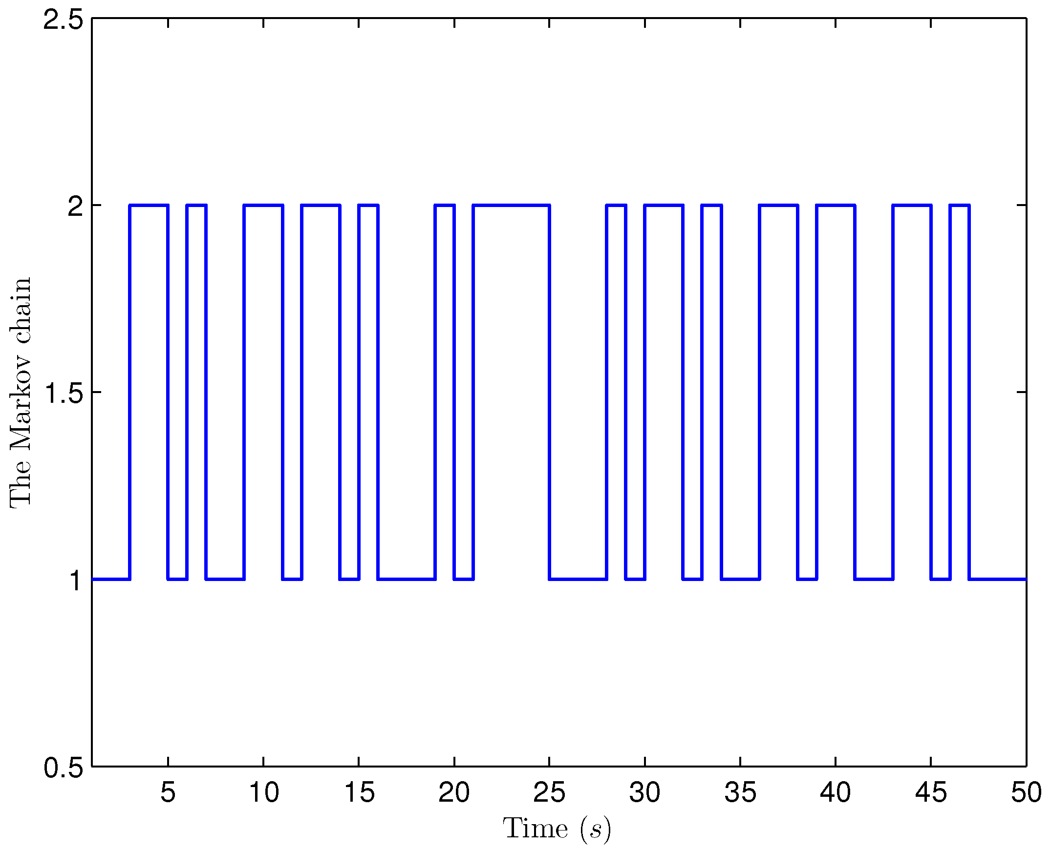
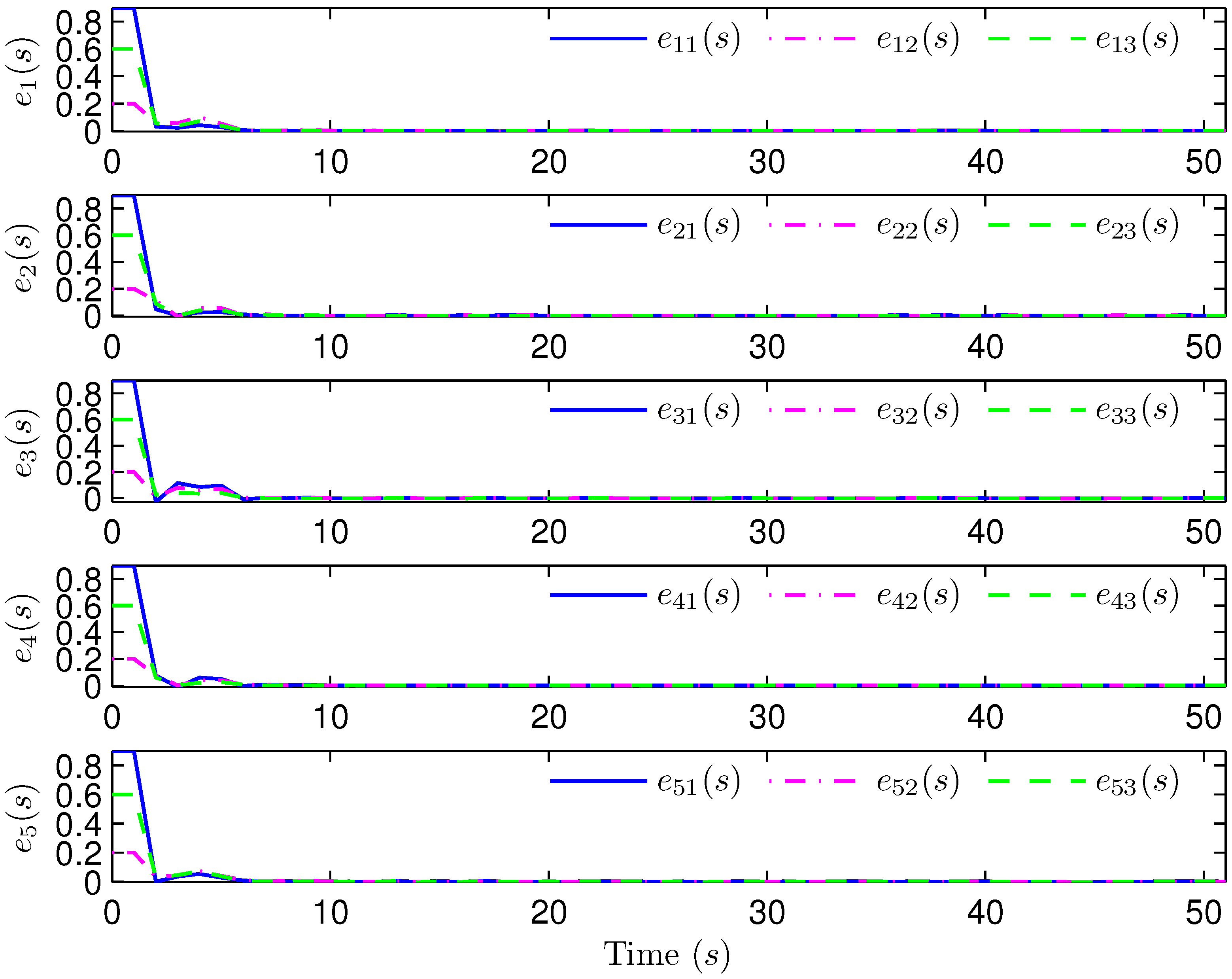
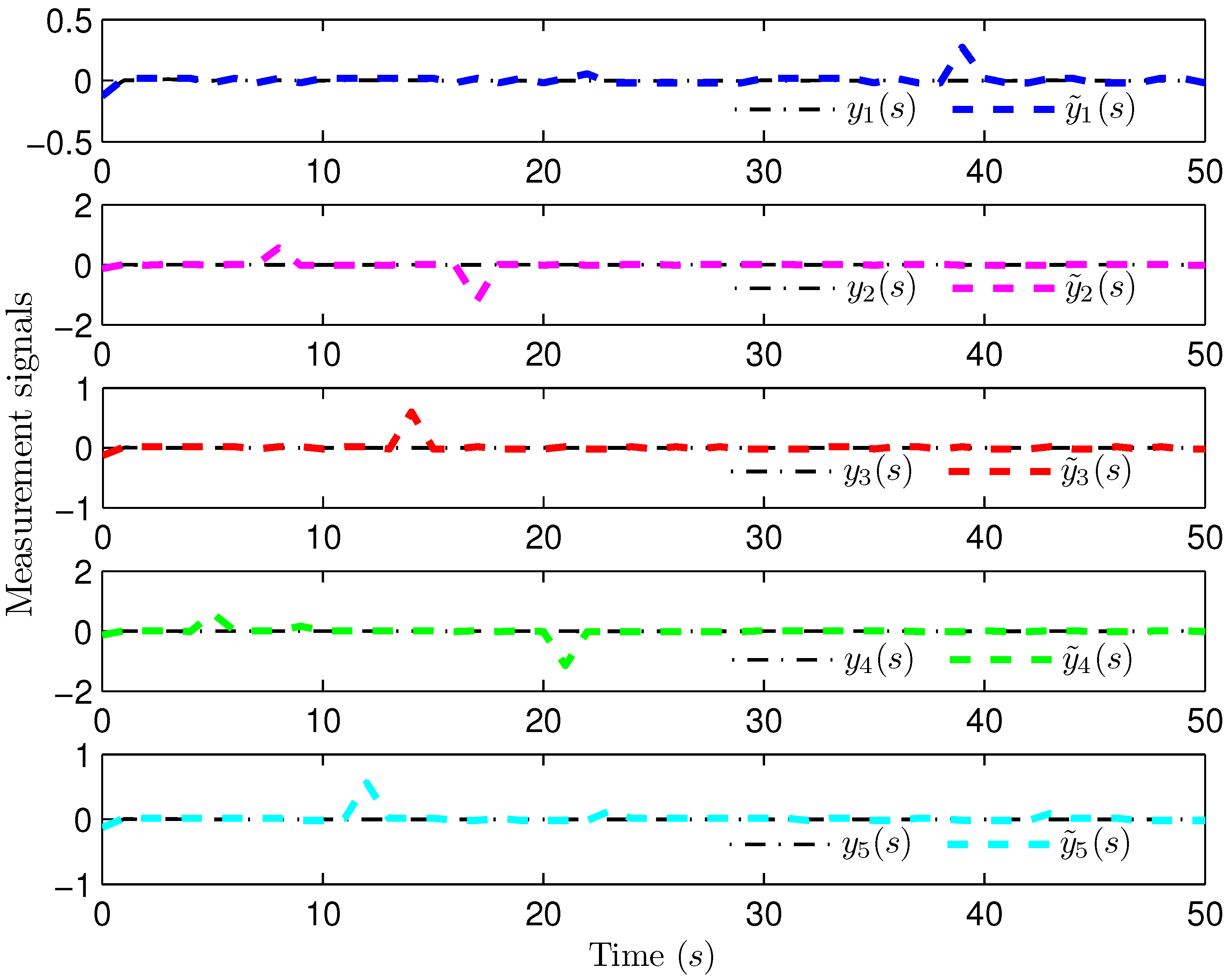
4. Simulation Examples

Example 1.

Consider a CN (1) ($U=5$) with the following parameters:

$$\begin{array}{cc}\hfill & p=2,M=6,q=0.01,\rho =0.0355,w_0=0.02,v_0=0.04,m=2,\overline{\mathcal{b}}=4,\underline{\mathcal{b}}=1,\hfill \\ \hfill & {\overline{϶}}_{11}={\overline{϶}}_{21}={\overline{϶}}_{31}={\overline{϶}}_{41}={\overline{϶}}_{51}=0.8,{\overline{϶}}_{12}={\overline{϶}}_{22}={\overline{϶}}_{32}={\overline{϶}}_{42}={\overline{϶}}_{52}=0.6,\rho =0.0355,\hfill \\ \hfill & {\pi }_{11}=0.55,{\pi }_{12}=0.45,{\pi }_{21}=0.4,{\pi }_{22}=0.6,D_1=D_2=0.03,D_3=D_4=0.02,\hfill \\ \hfill & {\mathrm{\Gamma }}^{\left(1\right)}=\mathrm{diag}\{0.52,0.53,0.52\},{\mathrm{\Gamma }}^{\left(2\right)}=\mathrm{diag}\{0.64,0.63,0.65\},m=1,n=0.3,D_5=0.01,\hfill \\ \hfill & {\mathrm{\Lambda }}^{\left(1\right)}=\left[\begin{array}{ccccc}-0.4& 0.15& 0.08& 0.12& 0.05\\ 0.15& -0.4& 0.1& 0.07& 0.08\\ 0.08& 0.1& -0.3& 0.04& 0.08\\ 0.12& 0.07& 0.04& -0.3& 0.07\\ 0.05& 0.08& 0.08& 0.07& -0.28\end{array}\right],{\mathrm{\Lambda }}^{\left(2\right)}=\left[\begin{array}{ccccc}-0.2& 0.05& 0.05& 0.05& 0.05\\ 0.05& -0.2& 0.05& 0.05& 0.05\\ 0.05& 0.05& -0.2& 0.05& 0.05\\ 0.05& 0.05& 0.05& -0.2& 0.05\\ 0.05& 0.05& 0.05& 0.05& -0.2\end{array}\right],\hfill \\ \hfill & A_1=A_2=\left[\begin{array}{ccc}0.01& 0& 0.009\\ 0& 0.001& 0.022\\ 0.011& 0.012& 0.018\end{array}\right],A_3=A_4=\left[\begin{array}{ccc}-0.02& -0.02& -0.01\\ 0.01& 0.03& -0.01\\ 0.03& 0.02& -0.01\end{array}\right],\kappa =0.01,\hfill \\ \hfill & A_5=\left[\begin{array}{ccc}-0.02& -0.01& -0.02\\ 0.01& 0.02& -0.03\\ -0.01& 0.04& -0.02\end{array}\right],B_{\mathcal{b}1}=B_{\mathcal{b}2}=\left[\begin{array}{ccc}0.02& -0.03& 0.01\\ 0.04& 0.01& 0.02\\ 0.02& -0.01& 0.03\end{array}\right],\hfill \\ \hfill & B_{\mathcal{b}3}=B_{\mathcal{b}4}=\left[\begin{array}{ccc}0.04& -0.01& 0.03\\ 0.02& 0.02& 0.02\\ 0.01& -0.02& 0.02\end{array}\right],B_{\mathcal{b}5}=\left[\begin{array}{ccc}0.02& -0.01& 0.02\\ 0.02& 0.03& 0.02\\ 0.02& -0.02& 0.04\end{array}\right],\hfill \\ \hfill & C_1=C_2=\left[\begin{array}{ccc}-0.1& 0.2& -0.1\end{array}\right],C_3=C_4=\left[\begin{array}{ccc}-0.1& 0.2& -0.1\end{array}\right],\hfill \\ \hfill & C_5=\left[\begin{array}{ccc}-0.1& 0.2& -0.1\end{array}\right],E_1=E_2=E_3=E_4=E_5=\left[\begin{array}{ccc}1& 1& 1\\ 1& 1& 1\\ 1& 1& 1\end{array}\right],\hfill \\ \hfill & F_1=F_2=\left[\begin{array}{c}0.01\\ 0.01\\ 0\end{array}\right],F_3=F_4=\left[\begin{array}{c}-0.01\\ -0.01\\ -0.01\end{array}\right],F_5=\left[\begin{array}{c}-0.02\\ -0.01\\ -0.02\end{array}\right].\hfill \end{array}$$

The nonlinear function $g\left(x_i\left(s\right)\right)$ ($i=1,2,\dots ,U)$ is chosen as follows:

$$\begin{array}{c}\hfill g\left(x_i\left(s\right)\right)=\left[\begin{array}{c}-0.06x_{i1}\left(s\right)+0.03x_{i2}\left(s\right)+\tanh \left(0.03x_{i1}\left(s\right)\right)\\ 0.06x_{i2}\left(s\right)-\tanh \left(0.02x_{i2}\left(s\right)\right)\\ -0.06x_{i2}\left(s\right)+0.03x_{i3}\left(s\right)+\tanh \left(0.03x_{i2}\left(s\right)\right)\end{array}\right]\end{array}$$

where $x_{i\sigma }\left(s\right)(\sigma =1,2,3)$ is the $\sigma$th element of $x_i\left(s\right)$. It can be observed that (3) is fulfilled as follows:

$$\begin{array}{cc}\hfill {\Xi }_1& =\left[\begin{array}{ccc}-0.06& 0.03& 0\\ 0& 0.04& 0\\ 0& -0.06& 0.03\end{array}\right]\mathit{and}{\Xi }_2=\left[\begin{array}{ccc}-0.03& 0.03& 0\\ 0& 0.06& 0\\ 0& -0.03& 0.03\end{array}\right].\hfill \end{array}$$

By solving the optimization issue (34) subject to matrix inequalities (31)–(33), the gain parameters of the estimator (8) are calculated as follows:

$$\begin{array}{cc}\hfill S_{11}& ={10}^{-14}\times \left[\begin{array}{c}0.1015\\ 0.0261\\ 0.2212\end{array}\right],S_{21}={10}^{-15}\times \left[\begin{array}{c}0.2787\\ -0.4131\\ 0.2407\end{array}\right],S_{31}={10}^{-16}\times \left[\begin{array}{c}0.7013\\ -0.7124\\ 0.0248\end{array}\right],\hfill \\ \hfill S_{41}& ={10}^{-17}\times \left[\begin{array}{c}0.2144\\ -0.2898\\ 0.1688\end{array}\right],S_{51}={10}^{-17}\times \left[\begin{array}{c}0.0952\\ -0.1899\\ 0.0227\end{array}\right],S_{12}={10}^{-15}\times \left[\begin{array}{c}0.1812\\ 0.0621\\ 0.1680\end{array}\right],\hfill \\ \hfill S_{22}& ={10}^{-18}\times \left[\begin{array}{c}0.6679\\ -0.8591\\ 0.7532\end{array}\right],S_{32}={10}^{-18}\times \left[\begin{array}{c}0.2586\\ -0.4815\\ 0.4934\end{array}\right],S_{42}={10}^{-16}\times \left[\begin{array}{c}-0.0004\\ 0.0001\\ 0.1626\end{array}\right],\hfill \\ \hfill S_{52}& ={10}^{-13}\times \left[\begin{array}{c}0.0879\\ -0.5279\\ 0.1690\end{array}\right].\hfill \end{array}$$

Select the initial conditions $x_i\left(\varsigma \right)={\left[\begin{array}{ccc}0.9& 0.2& 0.6\end{array}\right]}^T$ and ${\widehat{x}}_i\left(\varsigma \right)={\left[\begin{array}{ccc}0& 0& 0\end{array}\right]}^T$ ($\varsigma =-4,-3,\dots ,0,i=1,2,\dots ,5)$. Select $\mathcal{H}\left(s\right)=\cos (3s+1)$ and ${\mathcal{b}}_1\left(s\right)={\mathcal{b}}_2\left(s\right)=3+{(-1)}^s$. The simulation figures are presented in Figure 3, Figure 4, Figure 5, Figure 6 and Figure 7. Figure 3 shows the current mode describing randomly varying couplings, where “1” and “2” in the vertical coordinate represent the first and second mode of couplings, respectively. In Figure 4, the estimation error is represented by five nodes. Figure 4 shows that the estimation error for each node is low and gradually approximates to 0, which illustrates that the SE is exact. The original measurement signal and the one received by the estimator are plotted in Figure 5, and the deviation between them indicates the existence of random bit errors. Figure 6 depicts the norm of the estimation error (i.e., ${∥e\left(s\right)∥}^2$). From Figure 6, we see that ${∥e\left(s\right)∥}^2$ is bounded; that is, the estimator performance requirement (14) of exponential ultimate boundedness in mean square is fulfilled for CN (1). In Figure 7, the occurrence of random bit errors is revealed. For node 2, bit flipping occurs in the second bit and the first bit at time steps 8 and 17, respectively, which causes signal distortion at the same time steps in Figure 5. Furthermore, the higher bit undergoes bit flipping, and a larger deviation appears between the original measurement outputs and the received ones. In summary, the estimation results obtained by the designed non-fragile estimator are good.

Example 2.

For a delayed complex network (1) ($U=4$) whose local dynamical system ($l_x=3$) is a discrete-time Chua’s circuit (as is depicted in Figure 8), $x_1\left(s\right)$, $x_2\left(s\right)$ and $x_3\left(s\right)$ denote voltages $v_{C_1}$ and $v_{C_2}$ across the linear capacitors with capacitances $C_1$ and $C_2$, and the current $i_L$ passing the linear inductor L, respectively; and the nonlinear function $g(·)$ describes voltage versus the current feature of the nonlinear resistor $N_R$ (Chua’s diode) [5,69].

The parameters of such a complex network are presented as follows:

$$\begin{array}{cc}\hfill & \kappa =0.01,{\pi }_{11}=0.65,{\pi }_{12}=0.35,{\pi }_{21}=0.5,{\pi }_{22}=0.5,w_0=0.02,v_0=0.04,m=2,\hfill \\ \hfill & {\mathrm{\Lambda }}^{\left(1\right)}=\left[\begin{array}{cccc}-0.4& 0.15& 0.15& 0.1\\ 0.2& -0.6& 0.2& 0.2\\ 0.15& 0.15& -0.5& 0.2\\ 0.2& 0.2& 0.2& -0.6\end{array}\right],{\mathrm{\Lambda }}^{\left(2\right)}=\left[\begin{array}{cccc}-0.64& 0.22& 0.22& 0.2\\ 0.22& -0.58& 0.12& 0.24\\ 0.22& 0.12& -0.44& 0.1\\ 0.2& 0.24& 0.1& -0.54\end{array}\right],\hfill \\ \hfill & A_1=\left[\begin{array}{ccc}0.6& 0.4& 0\\ 0.3& 0.7& 0.2\\ 0& -5.4& 0.8\end{array}\right],A_2=A_1,A_3=\left[\begin{array}{ccc}0.8& 0.2& 0\\ 0.25& 0.75& 0.1\\ 0& -0.2& 0.9\end{array}\right],A_4=A_3,\hfill \\ \hfill & B_{\mathcal{b}1}=B_{\mathcal{b}2}=B_{\mathcal{b}3}=B_{\mathcal{b}4}=0.01I_{\left(3\right)},\rho =0.0355,{\overline{϶}}_{11}={\overline{϶}}_{21}={\overline{϶}}_{31}={\overline{϶}}_{41}=0.4,\hfill \\ \hfill & {\mathrm{\Gamma }}^{\left(1\right)}=I_{\left(3\right)},{\mathrm{\Gamma }}^{\left(2\right)}=0.5I_{\left(3\right)},q=0.01,m=I_{\left(2\right)},{\overline{϶}}_{12}={\overline{϶}}_{22}={\overline{϶}}_{32}={\overline{϶}}_{42}=0.5,M=6,\hfill \\ \hfill & C_1=C_2=C_3=C_4=\left[\begin{array}{ccc}1& 0& 0\\ 0& 1& 0\end{array}\right],D_1=\left[\begin{array}{c}0.003\\ 0.003\end{array}\right],D_3=\left[\begin{array}{c}0.002\\ 0.002\end{array}\right],n=\left[\begin{array}{cc}0.01& 0.01\\ 0.01& 0.01\end{array}\right],\hfill \\ \hfill & D_2=D_1,D_4=D_3,E_1=E_2=E_3=E_4=I_{\left(3\right)},F_1=F_2=F_3=F_4=I_{\left(3\right)},\underline{\mathcal{b}}=1,\overline{\mathcal{b}}=4.\hfill \end{array}$$

The expression of nonlinear function $g\left(x_i\left(s\right)\right)$ ($i=1,2,\dots ,4$) is

$$g\left(x_i\left(s\right)\right)=\left[\begin{array}{c}-0.2x_{i1}\left(s\right)+0.3\left(\right|x_{i1}\left(s\right)+2|-|x_{i1}\left(s\right)-2\left|\right)\\ 0\\ 0\end{array}\right],$$

and it was observed that ${\Xi }_1=\mathrm{diag}\{-0.8,0,0\}$ and ${\Xi }_2=\mathrm{diag}\{-0.2,0,0\}$ satisfy (3).

By solving the optimization issue (34), the gain parameters of estimator (8) are computed as follows:

$$\begin{array}{cc}\hfill & S_{11}={10}^{-7}\times \left[\begin{array}{cc}0.0098& -0.0376\\ 0.0292& -0.1120\\ 0.0125& -0.0480\end{array}\right],S_{21}={10}^{-8}\times \left[\begin{array}{cc}0.0064& 0.0365\\ 0.0182& 0.1017\\ 0.0032& -0.0254\end{array}\right],\hfill \\ \hfill & S_{31}={10}^{-12}\times \left[\begin{array}{cc}0.1480& -0.2986\\ -0.1049& -0.2305\\ -0.0446& -0.0712\end{array}\right],S_{41}={10}^{-12}\times \left[\begin{array}{cc}0.0064& -0.0917\\ -0.1303& -0.1586\\ -0.0650& 0.0492\end{array}\right],\hfill \\ \hfill & S_{12}={10}^{-9}\times \left[\begin{array}{cc}0.9808& 0.2382\\ -0.0243& -0.0038\\ -0.0124& -0.0011\end{array}\right],S_{22}={10}^{-12}\times \left[\begin{array}{cc}-0.3878& 0.6634\\ -0.2159& 0.5081\\ -0.2846& 0.7688\end{array}\right],\hfill \\ \hfill & S_{32}={10}^{-12}\times \left[\begin{array}{cc}-0.4269& 0.0116\\ -0.0791& -0.0603\\ -0.2546& 0.0351\end{array}\right],S_{42}={10}^{-9}\times \left[\begin{array}{cc}0.0189& 0.0205\\ 0.1827& 0.1960\\ 0.0793& 0.0852\end{array}\right].\hfill \end{array}$$

The initial states are given as $x_i(-4)={\left[\begin{array}{ccc}0.9& 0.2& 0.6\end{array}\right]}^T$, $x_i(-3)={\left[\begin{array}{ccc}0.8& 0.4& 0.2\end{array}\right]}^T$, $x_i(-2)={\left[\begin{array}{ccc}0.2& 0.7& 0.7\end{array}\right]}^T$, $x_i(-1)={\left[\begin{array}{ccc}0.3& 0.4& 0.2\end{array}\right]}^T$, $x_i\left(0\right)={\left[\begin{array}{ccc}0.4& 0.2& 0.1\end{array}\right]}^T$, ${\widehat{x}}_i(-4)={\left[\begin{array}{ccc}0.3& 0.4& 0.1\end{array}\right]}^T$, ${\widehat{x}}_i(-3)={\left[\begin{array}{ccc}0.5& 0.4& 0.2\end{array}\right]}^T$, ${\widehat{x}}_i(-2)={\left[\begin{array}{ccc}0.1& 0.6& 0.5\end{array}\right]}^T$, ${\widehat{x}}_i(-1)={\left[\begin{array}{ccc}0.3& 0.3& 0.3\end{array}\right]}^T$ and ${\widehat{x}}_i\left(0\right)={\left[\begin{array}{ccc}0.4& 0.5& 0.2\end{array}\right]}^T$ ($i=1,2,\dots ,4$). $\mathcal{H}\left(s\right)=0.01cos(3s+1)I_{\left(2\right)}$ and ${\mathcal{b}}_1\left(s\right)={\mathcal{b}}_2\left(s\right)=3+{(-1)}^s$ are chosen. Simulation curves are presented in Figure 9, Figure 10, Figure 11, Figure 12 and Figure 13. In Figure 9, the situation of mode switching is exhibited for the Markov chain, where “1” (or “2”) in the vertical coordinate indicates that coupling occurred with mode 1 (or mode 2). In Figure 10, the SE error $e_i\left(s\right)$ ($i=1,2,\dots ,4$) is presented, which is within the interval $[-2.645,3.012]$. In Figure 11, the ideal measurement signal and the actually received one are shown, and there is a difference between them. When an accurate description of the received measurement signal is provided, instead of using the ideal measurement signal, the estimation performance is guaranteed. In Figure 12, the norm of the SE error $e\left(s\right)$ is presented, which is bounded (not more than $11.92$). In Figure 13, for the BBS from measurement $y_{i♭}$ ($i=1,2,\dots ,4$, $♭=1,2$), bits that undergo flipping are presented. For the measurement component $y_{11}\left(s\right)$, bit flipping occurred in bits 5, 2, 6, 4, 6 and 2 at time steps 19, 22, 41, 45, 46 and 54, respectively. In light of the aforementioned outcomes, the developed non-fragile SE means presented in this paper are valid.

5. Conclusions

The issue of non-fragile SE was investigated in this paper for a type of nonlinear delayed CN with randomly varying couplings under BESs. A Markov chain was used to reflect the stochastic variations in both the network topology and the inner coupling, in combination with the Kronecker delta function. The BESs were applied to the signal transmission between the sensor and the remote state estimator. The phenomenon of random bit errors was considered and described using a sequence of Bernoulli-distributed random variables. Considering the gain perturbations that occurred during the practical execution of the estimator, the non-fragile state estimator was modelled under different gain variations, which ensured that the SE error dynamics were EUB in mean square and the ultimate bound was minimized. The gain parameter of the established estimator was obtained by tackling the optimization problem constrained by some linear matrix inequalities. The working ability of the designed estimator was demonstrated through two expository examples. In future, we would extend the acquired result to the SE of (1) CNs using the available measurement outputs from only a portion of the network nodes [70,71]; (2) sensor networks [72,73]; and (3) other systems [74,75].

References

1. Mei, Z.; Oguchi, T. A real-time identification method of network structure in complex network systems. Int. J. Syst. Sci. 2023, 54, 549–564. [Google Scholar] [CrossRef]
2. Shen, Y.; Wang, Z.; Dong, H.; Liu, H.; Chen, Y. Set-membership state estimation for multirate nonlinear complex networks under FlexRay protocols: A neural-network-based approach. IEEE Trans. Neural Netw. Learn. Syst. 2025, 36, 4922–4933. [Google Scholar] [CrossRef]
3. Shang, R.; Dong, H.; Wang, C.; Chen, S.; Sun, T.; Guan, C. Imbalanced data augmentation for pipeline fault diagnosis: A multi-generator switching adversarial network. Control Eng. Pract. 2024, 144, 105839. [Google Scholar] [CrossRef]
4. Shen, H.; Hu, X.; Wu, X.; He, S.; Wang, J. Generalized dissipative state estimation of singularly perturbed switched complex dynamic networks with persistent dwell-time mechanisms. IEEE Trans. Syst. Man, Cybern. Syst. 2022, 52, 1795–1806. [Google Scholar] [CrossRef]
5. Liu, Y.; Wang, Z.; Ma, L.; Alsaadi, F.E. A partial-nodes-based information fusion approach to state estimation for discrete-time delayed stochastic complex networks. Inf. Fusion 2019, 49, 240–248. [Google Scholar] [CrossRef]
6. Ma, X.; Zhou, H.; Li, Z. On the resilience of modern power systems: A complex network perspective. Renew. Sustain. Energy Rev. 2021, 152, 111646. [Google Scholar] [CrossRef]
7. Zhang, J.; Wang, J.-A.; Zhang, J.; Li, M.; Zhao, Z.; Wen, X. Fixed-time event-triggered pinning synchronization of complex network via aperiodically intermittent control. Neurocomputing 2024, 614, 128818. [Google Scholar] [CrossRef]
8. Wan, X.; Wang, Z.; Han, Q.; Wu, M. Finite-time H state estimation for discrete time-delayed genetic regulatory networks under stochastic communication protocols. IEEE Trans. Circuits Syst. Regul. Pap. 2018, 65, 3481–3491. [Google Scholar] [CrossRef]
9. Gao, Y.; Liu, J.; Wang, Z.; Wu, L. Interval type-2 FNN-based quantized tracking control for hypersonic flight vehicles with prescribed performance. IEEE Trans. Syst. Man, Cybern. Syst. 2021, 51, 1981–1993. [Google Scholar] [CrossRef]
10. Zhao, L.-H.; Wen, S.; Xu, M.; Shi, K.; Zhu, S.; Huang, T. PID control for output synchronization of multiple output coupled complex networks. IEEE Trans. Netw. Sci. Eng. 2022, 9, 1553–1566. [Google Scholar] [CrossRef]
11. Wu, Y.; Shen, B.; Ahn, C.K.; Li, W. Intermittent dynamic event-triggered control for synchronization of stochastic complex networks. IEEE Trans. Circuits Syst. Regul. Pap. 2021, 68, 2639–2650. [Google Scholar] [CrossRef]
12. Huang, C.; Cao, J.; Wen, F.; Yang, X. Stability analysis of SIR model with distributed delay on complex networks. PLoS ONE 2016, 11, e0158813. [Google Scholar] [CrossRef] [PubMed]
13. Li, Y.; Zhou, X.; Li, B. Existence and global exponential stability of Weyl almost automorphic solution in finite dimensional distributions for SDINNs. Int. J. Syst. Sci. 2025, 56, 561–581. [Google Scholar] [CrossRef]
14. Zhang, R.; Liu, H.; Liu, Y.; Tan, H. Dynamic event-triggered state estimation for discrete-time delayed switched neural networks with constrained bit rate. Syst. Sci. Control Eng. 2024, 12, 2334304. [Google Scholar] [CrossRef]
15. Hou, N.; Wang, Z.; Dong, H.; Hu, J.; Liu, X. Sensor fault estimation for nonlinear complex networks with time delays under saturated innovations: A binary encoding scheme. IEEE Trans. Netw. Sci. Eng. 2022, 9, 4171–4183. [Google Scholar] [CrossRef]
16. Hu, J.; Wang, Z.; Liu, G.-P.; Zhang, H. Variance-constrained recursive state estimation for time-varying complex networks with quantized measurements and uncertain inner coupling. IEEE Trans. Neural Netw. Learn. Syst. 2019, 31, 1955–1967. [Google Scholar] [CrossRef]
17. Feng, S.; Li, X.; Zhang, S.; Jian, Z.; Duan, H.; Wang, Z. A review: State estimation based on hybrid models of Kalman filter and neural network. Syst. Sci. Control Eng. 2023, 11, 2173682. [Google Scholar] [CrossRef]
18. Shen, Y.; Wang, Z.; Dong, H. Minimum-variance state and fault estimation for multirate systems with dynamical bias. IEEE Trans. Circuits Syst. II Express Briefs 2022, 69, 2361–2365. [Google Scholar] [CrossRef]
19. Li, Q.; Wang, Z.; Sheng, W.; Alsaadi, F.E.; Alsaadi, F.E. Dynamic event-triggered mechanism for H non-fragile state estimation of complex networks under randomly occurring sensor saturations. Inf. Sci. 2020, 509, 304–316. [Google Scholar] [CrossRef]
20. Liu, D.; Wang, Z.; Liu, Y.; Alsaadi, F.E.; Alsaadi, F.E. Recursive state estimation for stochastic complex networks under round-robin communication protocol: Handling packet disorders. IEEE Trans. Netw. Sci. Eng. 2021, 8, 2455–2468. [Google Scholar] [CrossRef]
21. Li, X.; Zhang, P.; Dong, H. A robust covert attack strategy for a class of uncertain cyber-physical systems. IEEE Trans. Autom. Control 2024, 69, 1983–1990. [Google Scholar] [CrossRef]
22. Ding, L.; Sun, W. Predefined time fuzzy adaptive control of switched fractional-order nonlinear systems with input saturation. Int. J. Netw. Dyn. Intell. 2023, 2, 100019. [Google Scholar] [CrossRef]
23. Wang, Y.-A.; Shen, B.; Zou, L.; Han, Q.-L. A survey on recent advances in distributed filtering over sensor networks subject to communication constraints. Int. J. Netw. Dyn. Intell. 2023, 2, 100007. [Google Scholar] [CrossRef]
24. Wang, Y.; Liu, H.-J.; Tan, H.-L. An overview of filtering for sampled-data systems under communication constraints. Int. J. Netw. Dyn. Intell. 2023, 2, 100011. [Google Scholar] [CrossRef]
25. Gao, Y.; Xiao, F.; Liu, J.; Wang, R. Distributed soft fault detection for interval type-2 fuzzy-model-based stochastic systems with wireless sensor networks. IEEE Trans. Ind. Inform. 2019, 15, 334–347. [Google Scholar] [CrossRef]
26. Wang, C.; Wang, Z.; Dong, H.; Lauria, S.; Liu, W.; Wang, Y.; Fadzil, F.; Liu, H. Fusionformer: A novel adversarial transformer utilizing fusion attention for multivariate anomaly detection. IEEE Trans. Neural Netw. Learn. Syst. 2025; in press. [Google Scholar] [CrossRef]
27. Li, H.; Li, X.; Sun, Y.; Dong, H.; Xu, G. First-arrival picking for out-of-distribution noisy data: A cost-effective transfer learning method with tens of samples. IEEE Trans. Geosci. Remote Sens. 2024, 62, 1–13. [Google Scholar] [CrossRef]
28. Song, J.; Zhou, S.; Niu, Y.; Cao, Z.; He, S. Anti-disturbance control for hidden Markovian jump systems: Asynchronous disturbance observer approach. IEEE Trans. Autom. Control 2023, 68, 6982–6989. [Google Scholar] [CrossRef]
29. Wang, X.F. Complex networks: Topology, dynamics and synchronization. Int. J. Bifurc. Chaos 2002, 12, 885–916. [Google Scholar] [CrossRef]
30. Gao, P.; Jia, C.; Zhou, A. Encryption-decryption-based state estimation for nonlinear complex networks subject to coupled perturbation. Syst. Sci. Control Eng. 2024, 12, 2357796. [Google Scholar] [CrossRef]
31. Yang, X.; Cao, J.; Lu, J. Synchronization of Markovian coupled neural networks with nonidentical node-delays and random coupling strengths. IEEE Trans. Neural Netw. Learn. Syst. 2011, 60–71. [Google Scholar] [CrossRef]
32. Gao, C.; Guo, B.; Xiao, Y.; Bao, J. Aperiodically synchronization of multi-links delayed complex networks with semi-Markov jump and their numerical simulations to single-link robot arms. Neurocomputing 2024, 575, 127286. [Google Scholar] [CrossRef]
33. Hu, J.; Wang, Z.; Liu, G.-P. Delay compensation-based state estimation for time-varying complex networks with incomplete observations and dynamical bias. IEEE Trans. Cybern. 2022, 52, 12071–12083. [Google Scholar] [CrossRef] [PubMed]
34. Shen, B.; Wang, Z.; Ding, D.; Shu, H. H state estimation for complex networks with uncertain inner coupling and incomplete measurements. IEEE Trans. Neural Netw. Learn. Syst. 2013, 24, 2027–2037. [Google Scholar] [CrossRef]
35. Leung, H.; Seneviratne, C.; Xu, M. A novel statistical model for distributed estimation in wireless sensor networks. IEEE Trans. Signal Process. 2015, 63, 3154–3164. [Google Scholar] [CrossRef]
36. Huo, N.; Shen, D. Encoding-decoding mechanism-based finite-level quantized iterative learning control with random data dropouts. IEEE Trans. Autom. Sci. Eng. 2019, 17, 1343–1360. [Google Scholar] [CrossRef]
37. Yang, F.; Li, J.; Dong, H.; Shen, Y. Proportional-integral-type estimator design for delayed recurrent neural networks under encoding-decoding mechanism. Int. J. Syst. Sci. 2022, 53, 2729–2741. [Google Scholar] [CrossRef]
38. Zou, L.; Wang, Z.; Shen, B.; Dong, H. Secure recursive state estimation of networked systems against eavesdropping: A partial-encryption-decryption method. IEEE Trans. Autom. Control, 2024; in press. [Google Scholar] [CrossRef]
39. Zou, L.; Wang, Z.; Shen, B.; Dong, H. Encryption-decryption-based state estimation with multirate measurements against eavesdroppers: A recursive minimum-variance approach. IEEE Trans. Autom. Control 2023, 68, 8111–8118. [Google Scholar] [CrossRef]
40. Zou, L.; Wang, Z.; Shen, B.; Dong, H. Recursive state estimation in relay channels with enhanced security against eavesdropping: An Innovative encryption-decryption framework. Automatica 2025, 174, 112159. [Google Scholar] [CrossRef]
41. Liang, X.; Xu, J. Control for networked control systems with remote and local controllers over unreliable communication channel. Automatica 2018, 98, 86–94. [Google Scholar] [CrossRef]
42. Li, J.; Wang, Z.; Dong, H.; Fei, W. Delay-distribution-dependent state estimation for neural networks under stochastic communication protocol with uncertain transition probabilities. Neural Netw. 2020, 130, 143–151. [Google Scholar] [CrossRef]
43. Jin, Y.; Ma, X.; Meng, X.; Chen, Y. Distributed fusion filtering for cyber-physical systems under Round-Robin protocol: A mixed H2/H framework. Int. J. Syst. Sci. 2023, 54, 1661–1675. [Google Scholar] [CrossRef]
44. Geng, H.; Wang, Z.; Chen, Y.; Yi, X.; Cheng, Y. Variance-constrained filtering fusion for nonlinear cyber-physical systems with the denial-of-service attacks and stochastic communication protocol. IEEE/CAA J. Autom. Sin. 2022, 9, 978–989. [Google Scholar] [CrossRef]
45. Shen, Y.; Wang, Z.; Shen, B.; Dong, H. Outlier-resistant recursive filtering for multisensor multirate networked systems under weighted try-once-discard protocol. IEEE Trans. Cybern. 2020, 51, 4897–4908. [Google Scholar] [CrossRef] [PubMed]
46. Li, X.; Dong, H.; Wang, Z.; Han, F. Set-membership filtering for state-saturated systems with mixed time-delays under weighted try-once-discard protocol. IEEE Trans. Circuits Syst. II Express Briefs 2018, 66, 312–316. [Google Scholar] [CrossRef]
47. Hu, J.; Chen, W.; Wu, Z.; Chen, D.; Yi, X. Design of protocol-based finite-time memory fault detection scheme with circuit system application. IEEE Trans. Syst. Man Cybern. Syst. 2024, 54, 3110–3123. [Google Scholar] [CrossRef]
48. Han, F.; Wang, Z.; Dong, H.; Alsaadi, F.E.; Alharbi, K.H. A local approach to distributed H-consensus state estimation over sensor networks under hybrid attacks: Dynamic event-triggered scheme. IEEE Trans. Signal Inf. Process. Over Netw. 2022, 8, 556–570. [Google Scholar] [CrossRef]
49. Wu, W.; Yan, H.; Wang, Y.; Li, Z.; Wang, M. Fixed time cluster consensus for nonlinear multiagent systems by double dynamic event-triggered mechanisms. Int. J. Syst. Sci. 2024, 55, 3322–3336. [Google Scholar] [CrossRef]
50. Hu, J.; Hu, Z.; Caballero-Aguila, R.; Chen, C.; Fan, S.; Yi, X. Distributed resilient fusion filtering for nonlinear systems with multiple missing measurements via dynamic event-triggered mechanism. Inf. Sci. 2023, 637, 118950. [Google Scholar] [CrossRef]
51. Wang, W.; Ma, L.; Rui, Q.; Gao, C. A survey on privacy-preserving control and filtering of networked control systems. Int. J. Syst. Sci. 2024, 55, 2269–2288. [Google Scholar] [CrossRef]
52. Li, J.; Wang, Z.; Dong, H.; Yi, X. Outlier-resistant observer-based control for a class of networked systems under encoding-decoding mechanism. IEEE Syst. J. 2020, 16, 922–932. [Google Scholar] [CrossRef]
53. Gao, Y.; Hu, J.; Chi, K.; Jia, C.; Qi, J. A variance-constrained method to encoding-decoding H state estimation for memristive neural networks with energy harvesting sensor. Neurocomputing 2024, 579, 127448. [Google Scholar] [CrossRef]
54. Jin, F.; Ma, L.; Zhao, C.; Liu, Q. A quantization-coding scheme with variable data rates for cyber-physical systems under DoS attacks. Syst. Sci. Control Eng. 2024, 12, 2348690. [Google Scholar] [CrossRef]
55. Li, W.; Hou, N.; Yang, F.; Bu, X.; Sun, L. Finite-horizon variance-constrained H estimation for complex networks subject to dynamical bias using binary encoding schemes. IEEE Access 2023, 11, 142589–142600. [Google Scholar] [CrossRef]
56. Liu, Q.; Wang, Z.; Dong, H.; Jiang, C. Remote estimation for energy harvesting systems under multiplicative noises: A binary encoding scheme with probabilistic bit flips. IEEE Trans. Autom. Control 2022, 68, 343–354. [Google Scholar] [CrossRef]
57. Wen, P.; Dong, H.; Huo, F.; Li, J.; Lu, X. Observer-based PID control for actuator-saturated systems under binary encoding scheme. Neurocomputing 2022, 99, 54–62. [Google Scholar] [CrossRef]
58. Chen, W.; Wang, Z.; Ding, D.; Dong, H. Consensusability of discrete-time multi-agent systems under binary encoding with bit errors. Automatica 2021, 133, 109867. [Google Scholar] [CrossRef]
59. Wang, S.; Wang, Z.; Dong, H.; Chen, Y. A dynamic event-triggered approach to recursive nonfragile filtering for complex networks with sensor saturations and switching topologies. IEEE Trans. Cybern. 2022, 52, 11041–11054. [Google Scholar] [CrossRef]
60. Zhao, D.; Wang, Z.; Wei, G.; Liu, X. Nonfragile H state estimation for recurrent neural networks with time-varying delays: On proportional-integral observer design. IEEE Trans. Neural Netw. Learn. Syst. 2021, 32, 3553–3565. [Google Scholar] [CrossRef]
61. Xu, B.; Hu, X.; Li, S. Secure state estimation of memristive neural networks with dynamic self-triggered strategy subject to deception attacks. Neurocomputing 2024, 601, 128142. [Google Scholar] [CrossRef]
62. Zhuang, J.; Peng, S.; Peng, H. Non-fragile exponential synchronisation of stochastic neural networks via aperiodic intermittent impulsive control. Int. J. Syst. Sci. 2024, 55, 1021–1036. [Google Scholar] [CrossRef]
63. Zhang, S.; Wang, Z.; Ding, D.; Dong, H.; Alsaadi, F.E.; Hayat, T. Nonfragile H fuzzy filtering with randomly occurring gain variations and channel fadings. IEEE Trans. Fuzzy Syst. 2015, 24, 505–518. [Google Scholar] [CrossRef]
64. Bu, X.; Dong, H.; Wang, Z.; Liu, H. Non-fragile distributed fault estimation for a class of nonlinear time-varying systems over sensor networks: The finite-horizon case. IEEE Trans. Signal Inf. Process. Over Netw. 2018, 5, 61–69. [Google Scholar] [CrossRef]
65. Liu, Q.; Wang, Z.; He, X.; Ghinea, G.; Alsaadi, F.E. A resilient approach to distributed filter design for time-varying systems under stochastic nonlinearities and sensor degradation. IEEE Trans. Signal Process. 2016, 65, 1300–1309. [Google Scholar] [CrossRef]
66. Li, X.; Song, J.; Hou, N.; Dai, D.; Yang, F. Finite-horizon distributed set-membership filtering with dynamical bias and DoS attacks under binary encoding schemes. Inf. Sci. 2023, 641, 119084. [Google Scholar] [CrossRef]
67. Liu, Q.; Wang, Z. Moving-horizon estimation for linear dynamic networks with binary encoding schemes. IEEE Trans. Autom. Control 2020, 66, 1763–1770. [Google Scholar] [CrossRef]
68. Liu, Y.; Wang, Z.; Liu, X. Global exponential stability of generalized recurrent neural networks with discrete and distributed delays. Neural Netw. 2006, 19, 667–675. [Google Scholar] [CrossRef]
69. Cruz-Hernández, C.; Romero-Haros, N. Communicating via synchronized time-delay Chua’s circuits. Commun. Nonlinear Sci. Numer. Simul. 2008, 13, 645–659. [Google Scholar] [CrossRef]
70. Liu, Y.; Wang, Z.; Yuan, Y.; Liu, W. Event-triggered partial-nodes-based state estimation for delayed complex networks with bounded distributed delays. IEEE Trans. Syst. Man Cybern. Syst. 2017, 49, 1088–1098. [Google Scholar] [CrossRef]
71. Li, J.-Y.; Wang, Z.; Lu, R.; Xu, Y. Partial-nodes-based state estimation for complex networks with constrained bit rate. IEEE Trans. Netw. Sci. Eng. 2021, 8, 1887–1899. [Google Scholar] [CrossRef]
72. Han, F.; Wang, Z.; Liu, H.; Dong, H.; Lu, G. Local design of distributed state estimators for linear discrete time-varying systems over binary sensor networks: A set-membership approach. IEEE Trans. Syst. Man, Cybern. Syst. 2024, 54, 5641–5654. [Google Scholar] [CrossRef]
73. Hu, J.; Li, J.; Yan, H.; Liu, H. Optimized distributed filtering for saturated systems with amplify-and-forward relays over sensor networks: A dynamic event-triggered approach. IEEE Trans. Neural Netw. Learn. Syst. 2024, 35, 17742–17753. [Google Scholar] [CrossRef] [PubMed]
74. Song, J.; Wang, Y.-K.; Niu, Y.; Lam, H.-K.; He, S.; Liu, H. Periodic event-triggered terminal sliding mode speed control for networked PMSM system: A GA-optimized extended state observer approach. IEEE/ASME Trans. Mechatronics 2022, 27, 4153–4164. [Google Scholar] [CrossRef]
75. Liang, X.; Xu, J.; Wang, H.; Zhang, H. Decentralized output-feedback control with asymmetric one-step delayed information. IEEE Trans. Autom. Control 2023, 68, 7871–7878. [Google Scholar] [CrossRef]
Figure 1. The set of quantization values ( O ).
Sensors 25 02880 g001
Figure 2. The diagram of state estimation (SE) for complex network (CN) (1).
Sensors 25 02880 g002
Figure 3. Mode evolution.
Sensors 25 02880 g003
Figure 4. State estimation error of five nodes.
Sensors 25 02880 g004
Figure 5. The ideal and received measurement outputs.
Sensors 25 02880 g005
Figure 6. The norm of the estimation error e ( s ) .
Sensors 25 02880 g006
Figure 7. The occurrence of random bit errors.
Sensors 25 02880 g007
Figure 8. Chua’s circuit.
Sensors 25 02880 g008
Figure 9. Mode evolution.
Sensors 25 02880 g009
Figure 10. State estimation error of four nodes.
Sensors 25 02880 g010
Figure 11. The measurement output and the estimator input.
Sensors 25 02880 g011
Figure 12. The norm of the estimation error e ( s ) .
Sensors 25 02880 g012
Figure 13. The occurrence of random bit errors.
Sensors 25 02880 g013
Disclaimer/Publisher’s Note: The statements, opinions and data contained in all publications are solely those of the individual author(s) and contributor(s) and not of MDPI and/or the editor(s). MDPI and/or the editor(s) disclaim responsibility for any injury to people or property resulting from any ideas, methods, instructions or products referred to in the content.