
Detection and Mitigation of GNSS Gross Errors Utilizing the CEEMD and IQR Methods to Determine Sea Surface Height Using GNSS Buoys

Abstract
1. Introduction
2. Theory and Method
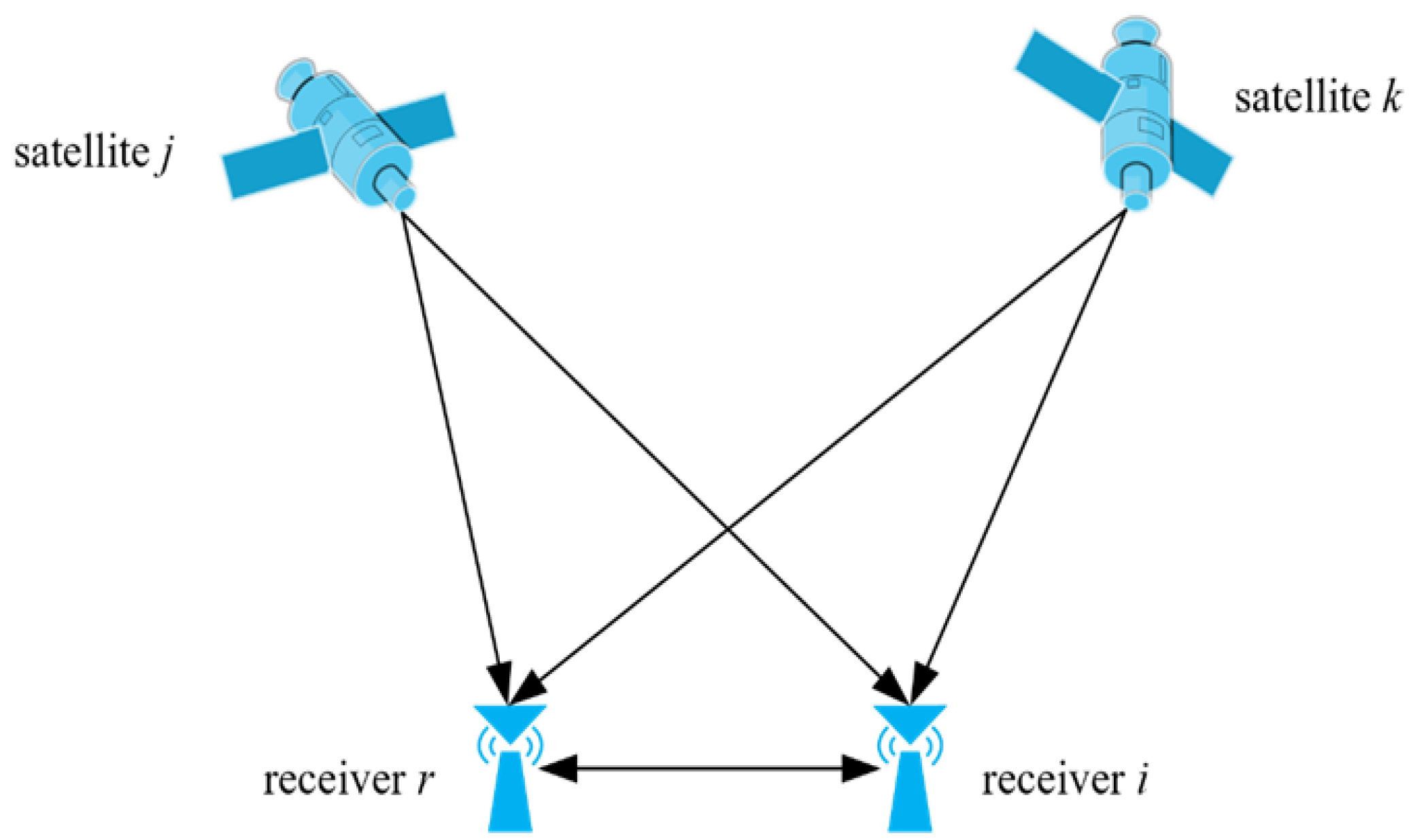
2.1. Determining Sea Surface Height Using GNSS RTK Technology
2.2. IQR Gross Error Detection Method
2.3. CEEMD Method
- (1)
- A pair of opposite white noise signals are added into the raw signal to derive the new signals and :
- (2)
- The signals and are decomposed into IMF components, respectively, using the EMD method:
- (3)
- The mean of the IMF components is computed with groups of noisy signals to achieve the final CEEMD result:
2.4. Enhanced IQR Gross Error Detection Algorithm Based on the CEEMD Method
- (1)
- The 3 criterion method is utilized to eliminate large deviations in the raw coordinate time series , preventing interference with CEEMD and reconstruction. For the outage values after eliminating gross errors, the mean interpolation method is employed to obtain a temporally continuous and complete coordinate sequence :
- (2)
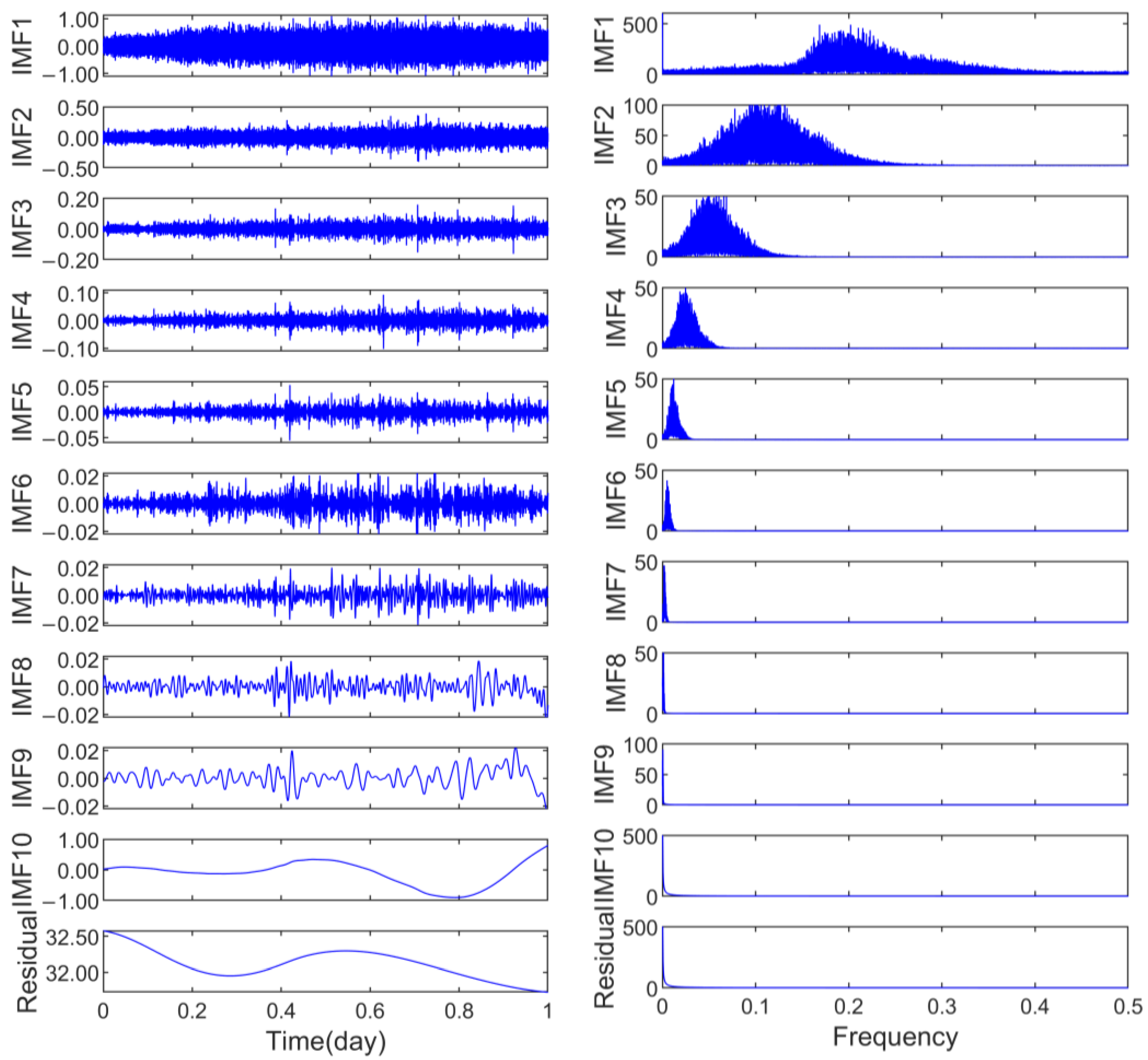
- The CEEMD method is used to decompose and extract the high-frequency noise signals as the residual time series. For the CEEMD and reconstruction process, an appropriate method should be adopted to select the IMF components. Based on previous research, the correlation coefficient method was utilized for signal–noise separation [46]. The correlation coefficient between the IMF components and the coordinate time series can be expressed as follows:where is the jth IMF component; represents the length of the coordinate time series data; and and denote the mean values of and . The IMF component , corresponding to the first local minimum among the correlation coefficients, is considered the boundary between noise and signal.
- (3)
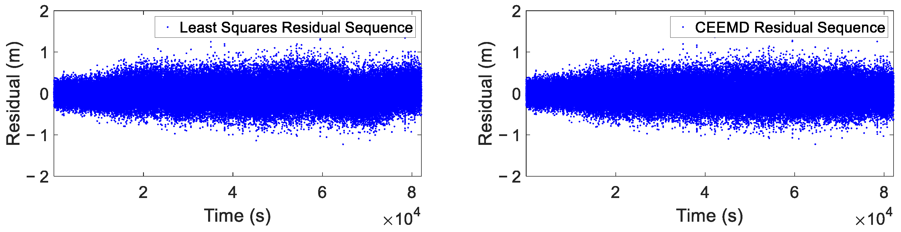
- The reconstruction with IMF components involves reconstructing the periodic signal of the coordinate time series with the components from to . After subtracting the periodic component and the trend component in , the residual time series R(t) is obtained:
- (4)
- Gross errors are detected in the residual time series using the IQR method. According to the IQR criterion, when the observed value is less than or greater than , it is considered a gross error and must be removed. The approach using steps (1) to (4) was named the CEEMD-IQR method and identifies all the gross errors in GNSS coordinate time series. The detailed data processing procedure is illustrated in Figure 2.
3. Experiment and Results
3.1. Validation with Simulated Data
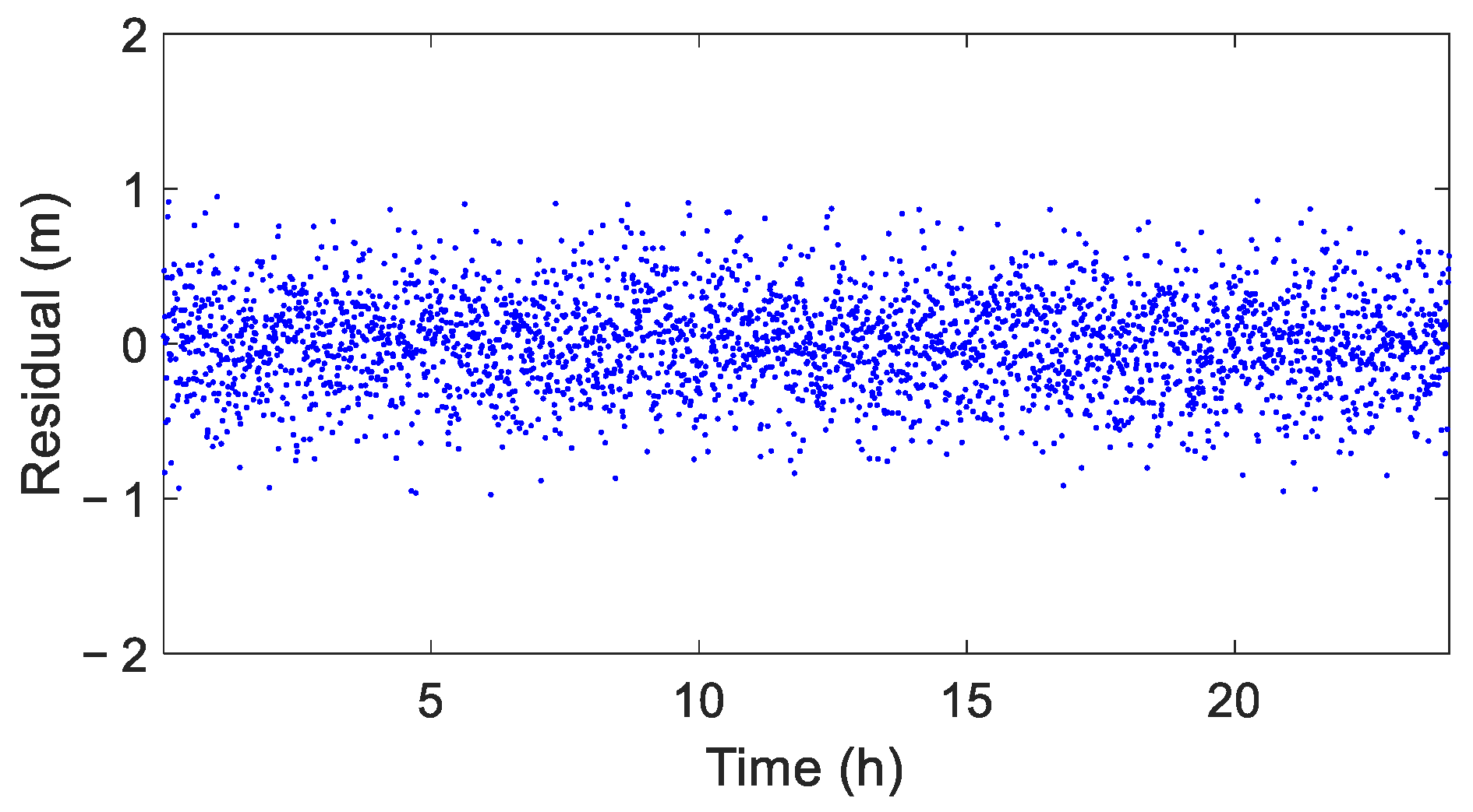
3.1.1. Generation of Simulation Data
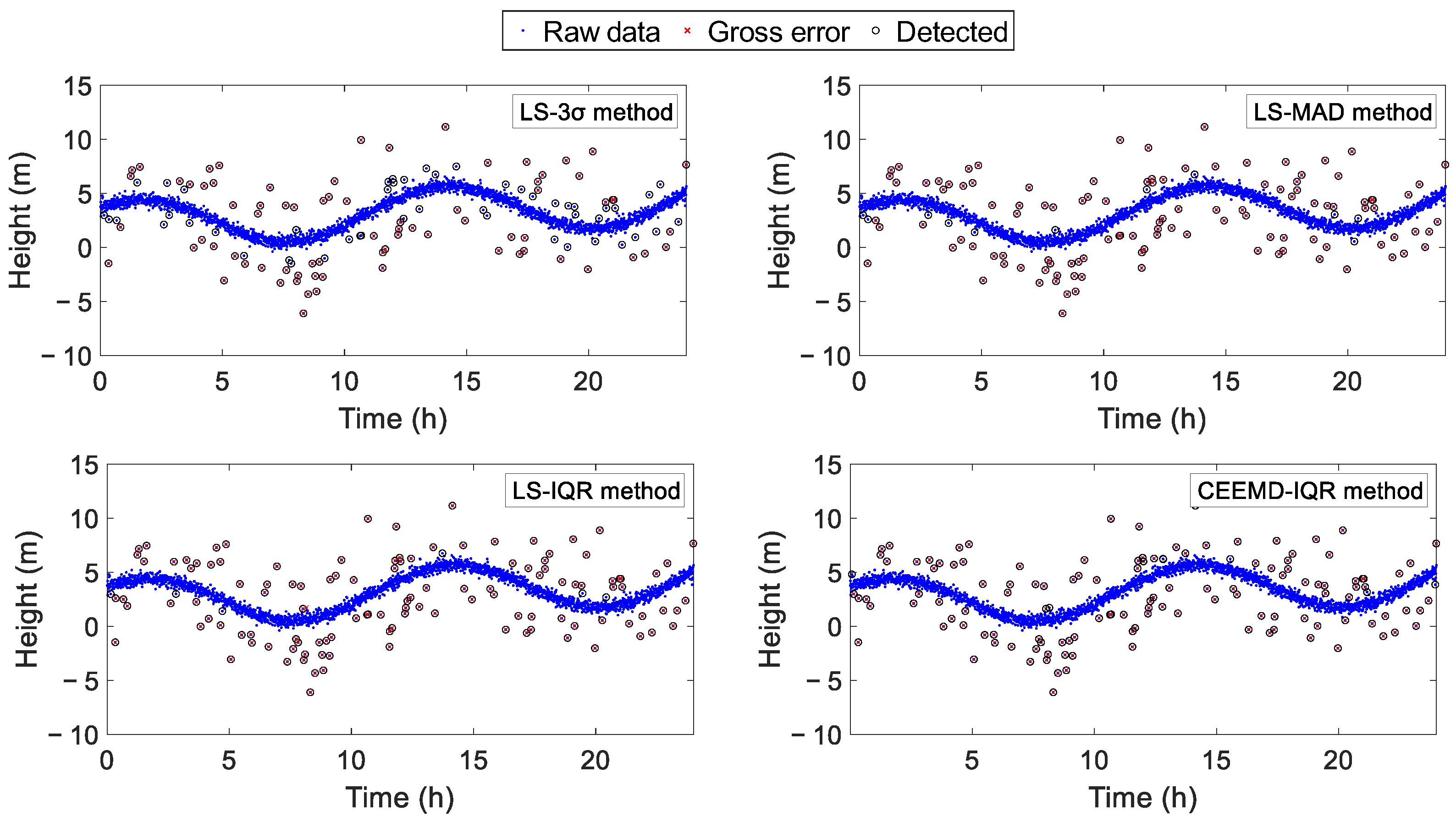
3.1.2. Analysis of Simulated Data
3.2. Analysis of Measured Data from GNSS Buoys
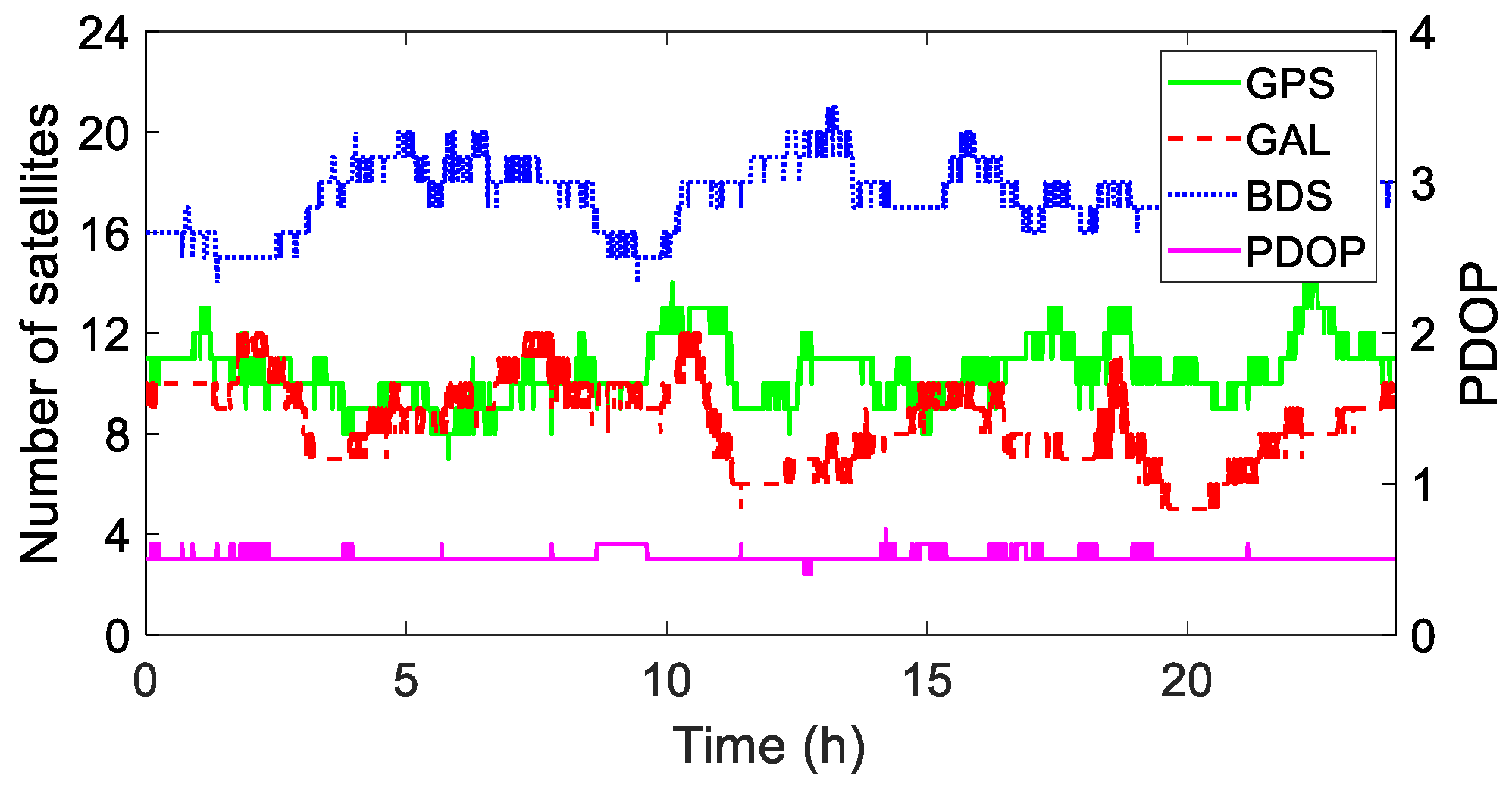
3.2.1. Acquisition of Measured Data
3.2.2. Detection of Gross Errors in GNSS Buoy Data
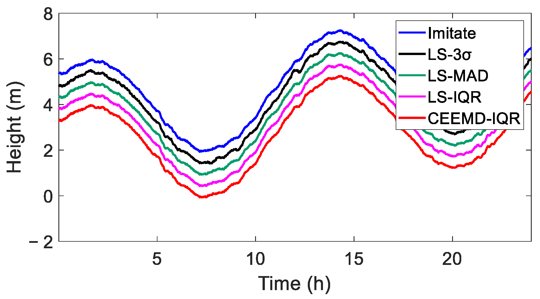
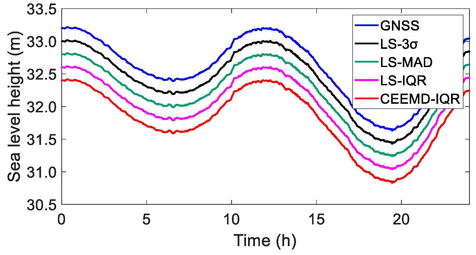
3.3. Analysis of the Sea Surface Height Accuracy Using GNSS Buoys
4. Conclusions
Author Contributions
Funding
Institutional Review Board Statement
Informed Consent Statement
Data Availability Statement
Acknowledgments
Conflicts of Interest
References
- Shen, C.; Zheng, W.; Shi, H.; Ding, D.; Wang, Z. Assessment and Regulation of Ocean Health Based on Ecosystem Services: Case Study in the Laizhou Bay, China. Acta Oceanol. Sin. 2015, 34, 61–66. [Google Scholar] [CrossRef]
- Wu, L.; Zhuang, S. Experimental Investigation of Effect of Tide on Coastal Groundwater Table. J. Hydrodyn. 2010, 22, 66–72. [Google Scholar] [CrossRef]
- Jacobi, M. Autonomous Inspection of Underwater Structures. Robot. Auton. Syst. 2015, 67, 80–86. [Google Scholar] [CrossRef]
- Xing, Q.; Wu, L.; Tian, L.; Cui, T.; Li, L.; Kong, F.; Gao, X.; Wu, M. Remote Sensing of Early-Stage Green Tide in the Yellow Sea for Floating-Macroalgae Collecting Campaign. Mar. Pollut. Bull. 2018, 133, 150–156. [Google Scholar] [CrossRef]
- Maldonado, J. A Multiple Knowledge Approach for Adaptation to Environmental Change: Lessons Learned from Coastal Louisiana’s Tribal Communities. J. Political Ecol. 2014, 21, 61–82. [Google Scholar] [CrossRef]
- Cheng, Y.; Ezer, T.; Atkinson, L.P.; Xu, Q. Analysis of Tidal Amplitude Changes Using the EMD Method. Cont. Shelf Res. 2017, 148, 44–52. [Google Scholar] [CrossRef]
- Kong, Q.; Guo, J.; Sun, Y.; Zhao, C.; Chen, C. Centimeter-Level Precise Orbit Determination for the HY-2A Satellite Using DORIS and SLR Tracking Data. Acta Geophys. 2017, 65, 1–12. [Google Scholar] [CrossRef]
- Guerra, M.; Hay, A.E.; Karsten, R.; Trowse, G.; Cheel, R.A. Turbulent Flow Mapping in a High-Flow Tidal Channel Using Mobile Acoustic Doppler Current Profilers. Renew. Energy 2021, 177, 759–772. [Google Scholar] [CrossRef]
- Revollo Sarmiento, G.N.; Revollo Sarmiento, N.V.; Delrieux, C.A.; Perillo, G.M.E. Morphological Characterization of Ponds and Tidal Courses in Coastal Wetlands Using Google Earth Imagery. Estuar. Coast. Shelf Sci. 2020, 246, 107041. [Google Scholar] [CrossRef]
- Han, S.; Ghobadi-Far, K.; Ray, R.D.; Papanikolaou, T. Tidal Geopotential Dependence on Earth Ellipticity and Seawater Density and Its Detection With the GRACE Follow-On Laser Ranging Interferometer. J. Geophys. Res. Oceans 2020, 125, e2020JC016774. [Google Scholar] [CrossRef]
- Yang, L.; Xu, Y.; Zhou, X.; Zhu, L.; Jiang, Q.; Sun, H.; Chen, G.; Wang, P.; Mertikas, S.P.; Fu, Y.; et al. Calibration of an Airborne Interferometric Radar Altimeter over the Qingdao Coast Sea, China. Remote Sens. 2020, 12, 1651. [Google Scholar] [CrossRef]
- Liu, Z.; Zheng, W.; Wu, F.; Kang, G.; Li, Z.; Wang, Q.; Cui, Z. Increasing the Number of Sea Surface Reflected Signals Received by GNSS-Reflectometry Altimetry Satellite Using the Nadir Antenna Observation Capability Optimization Method. Remote Sens. 2019, 11, 2473. [Google Scholar] [CrossRef]
- Yu, K. Tsunami-Wave Parameter Estimation Using GNSS-Based Sea Surface Height Measurement. IEEE Trans. Geosci. Remote Sens. 2015, 53, 2603–2611. [Google Scholar] [CrossRef]
- Purnell, D.; Gomez, N.; Chan, N.H.; Strandberg, J.; Holland, D.M.; Hobiger, T. Quantifying the Uncertainty in Ground-Based GNSS-Reflectometry Sea Level Measurements. IEEE J. Sel. Top. Appl. Earth Obs. Remote Sens. 2020, 13, 4419–4428. [Google Scholar] [CrossRef]
- Strandberg, J.; Hobiger, T.; Haas, R. Real-Time Sea-Level Monitoring Using Kalman Filtering of GNSS-R Data. GPS Solut. 2019, 23, 61. [Google Scholar] [CrossRef]
- Zhang, S.; Liu, K.; Liu, Q.; Zhang, C.; Zhang, Q.; Nan, Y. Tide Variation Monitoring Based Improved GNSS-MR by Empirical Mode Decomposition. Adv. Space Res. 2019, 63, 3333–3345. [Google Scholar] [CrossRef]
- Wang, X.; He, X.; Zhang, Q. Evaluation and Combination of Quad-Constellation Multi-GNSS Multipath Reflectometry Applied to Sea Level Retrieval. Remote Sens. Environ. 2019, 231, 111229. [Google Scholar] [CrossRef]
- Liang, G.; Li, S.; Bao, K.; Wang, G.; Teng, F.; Zhang, F.; Wang, Y.; Guan, S.; Wei, Z. Development of GNSS Buoy for Sea Surface Elevation Observation of Offshore Wind Farm. Remote Sens. 2023, 22, 5323. [Google Scholar] [CrossRef]
- Moore, T.; Zhang, K.; Close, G.; Moore, R. Real-Time River Level Monitoring Using GPS Heighting. GPS Solut. 2000, 4, 63–67. [Google Scholar] [CrossRef]
- Kotsakis, C.; Katsambalos, K.; Ampatzidis, D.; Gianniou, M. Evaluation of EGM08 Using GPS and Leveling Heights in Greece. In Gravity, Geoid and Earth Observation. International Association of Geodesy Symposia; Mertikas, S.P., Ed.; Springer: Berlin/Heidelberg, Germany, 2010; Volume 135, pp. 481–488. ISBN 978-3-642-10633-0. [Google Scholar]
- Church, J.A.; White, N.J. Sea-Level Rise from the Late 19th to the Early 21st Century. Surv. Geophys. 2011, 32, 585–602. [Google Scholar] [CrossRef]
- Simav, M.; Yildiz, H.; Türkezer, A.; Lenk, O.; Özsoy, E. Sea Level Variability at Antalya and Menteş Tide Gauges in Turkey: Atmospheric, Steric and Land Motion Contributions. Stud. Geophys. Geod. 2012, 56, 215–230. [Google Scholar] [CrossRef]
- Bos, M.S.; Fernandes, R.M.; Vethamony, P.; Mehra, P. Estimating Absolute Sea Level Variations by Combining GNSS and Tide Gauge Data. Indian J. Mar. Sci. 2014, 43, 1327–1331. [Google Scholar]
- Alothman, A.O.; Bos, M.; Fernandes, R.; Radwan, A.M.; Rashwan, M. Annual Sea Level Variations in the Red Sea Observed Using GNSS. Geophys. J. Int. 2020, 221, 826–834. [Google Scholar] [CrossRef]
- Wang, X.; He, X.; Shi, J.; Chen, S.; Niu, Z. Estimating Sea Level, Wind Direction, Significant Wave Height, and Wave Peak Period Using a Geodetic GNSS Receiver. Remote Sens. Environ. 2022, 279, 113135. [Google Scholar] [CrossRef]
- Wei, H.; Xiao, G.; Zhou, P.; Li, P.; Xiao, Z.; Zhang, B. Combining Galileo HAS and Beidou PPP-B2b with Helmert Coordinate Transformation Method. GPS Solut. 2025, 29, 35. [Google Scholar] [CrossRef]
- Estey, L.H.; Meertens, C.M. TEQC: The Multi-Purpose Toolkit for GPS/GLONASS Data. GPS Solut. 1999, 3, 42–49. [Google Scholar] [CrossRef]
- Xu, T.; Zhang, Z.; He, X.; Yuan, H. A Multi-cycle Slip Detection and Repair Method for Single-Frequency GNSS Receiver. Geomat. Inf. Sci. Wuhan Univ. 2024, 49, 465–472. [Google Scholar] [CrossRef]
- Gökalp, E.; Guengoer, O.; Boz, Y. Evaluation of Different Outlier Detection Methods for GPS Networks. Sensors 2008, 8, 7344–7358. [Google Scholar] [CrossRef]
- Wang, B.; Yu, J.; Liu, C.; Li, M.; Zhu, B. Data Snooping Algorithm for Universal 3D Similarity Transformation Based on Generalized EIV Model. Measurement 2018, 119, 56–62. [Google Scholar] [CrossRef]
- Gazeaux, J.; Williams, S.; King, M.; Bos, M.; Dach, R.; Deo, M.; Moore, A.W.; Ostini, L.; Petrie, E.; Roggero, M.; et al. Detecting Offsets in GPS Time Series: First Results from the Detection of Offsets in GPS Experiment. JGR Solid Earth 2013, 118, 2397–2407. [Google Scholar] [CrossRef]
- Zhuang, Y.; Sun, X.; Li, Y.; Huai, J.; Hua, L.; Yang, X.; Cao, X.; Zhang, P.; Cao, Y.; Qi, L.; et al. Multi-Sensor Integrated Navigation/Positioning Systems Using Data Fusion: From Analytics-Based to Learning-Based Approaches. Inf. Fusion 2023, 95, 62–90. [Google Scholar] [CrossRef]
- Nikolaidis, R. Observation of Geodetic and Seismic Deformation with the Global Positioning System. Ph.D. Thesis, University of California, San Diego, CA, USA, 2002. [Google Scholar]
- Jiang, W.; Zhou, X. Effect of the Span of Australian GPS Coordinate Time Series in Establishing an Optimal Noise Model. Sci. China Earth Sci. 2015, 58, 523–539. [Google Scholar] [CrossRef]
- Klos, A.; Bogusz, J.; Figurski, M.; Kosek, W. On the Handling of Outliers in the GNSS Time Series by Means of the Noise and Probability Analysis. In IAG 150 Years. International Association of Geodesy Symposia; Rizos, C., Willis, P., Eds.; Springer International Publishing: Cham, Switzerland, 2015; Volume 143, pp. 657–664. ISBN 978-3-319-24603-1. [Google Scholar]
- Marques, C.; Ferreira, J.; Rocha, A.; Castanheira, J.; Melo-Gonçalves, P.; Vaz, N.; Dias, J. Singular spectrum analysis and forecasting of hydrological time series. Phys. Chem. Earth Parts A/B/C 2006, 31, 1172–1179. [Google Scholar] [CrossRef]
- Dragomiretskiy, K.; Zosso, D. Variational Mode Decomposition. IEEE Trans. Signal Process. 2014, 62, 531–544. [Google Scholar] [CrossRef]
- Mallat, S. A Wavelet Tour of Signal Processing; Springer Academic Press: Amsterdam, The Netherlands; Boston, MA, USA, 2008; ISBN 978-0-12-374370-1. [Google Scholar]
- Huang, N.E.; Shen, Z.; Long, S.R.; Wu, M.C.; Shih, H.H.; Zheng, Q.; Yen, N.-C.; Tung, C.C.; Liu, H.H. The Empirical Mode Decomposition and the Hilbert Spectrum for Nonlinear and Non- Stationary Time Series Analysis. Proc. Math. Phys. Eng. Sci. 1998, 454, 903–995. [Google Scholar] [CrossRef]
- Wu, Z.; Huang, N.E. Ensemble Empirical Mode Decomposition: A Noise-Assisted Data Analysis Method. Adv. Adapt. Data Anal. 2009, 1, 1–41. [Google Scholar] [CrossRef]
- Yeh, J.-R.; Shieh, J.-S.; Huang, N.E. Complementary Ensemble Empirical Mode Decomposition: A Novel Noise Enhanced Data Analysis Method. Adv. Adapt. Data Anal. 2010, 2, 135–156. [Google Scholar] [CrossRef]
- Torres, M.E.; Colominas, M.A.; Schlotthauer, G.; Flandrin, P. A Complete Ensemble Empirical Mode Decomposition with Adaptive Noise. In Proceedings of the 2011 IEEE International Conference on Acoustics, Speech and Signal Processing (ICASSP), Prague, Czech Republic, 22–27 May 2011; IEEE: Prague, Czech Republic, 2011; pp. 4144–4147. [Google Scholar]
- Li, Y.; Han, L.; Yi, L.; Zhong, S.; Chen, C. Feature Extraction and Improved Denoising Method for Nonlinear and Nonstationary High-Rate GNSS Coseismic Displacements Applied to Earthquake Focal Mechanism Inversion of the El Mayor–Cucapah Earthquake. Adv. Space Res. 2021, 68, 3971–3991. [Google Scholar] [CrossRef]
- Xiong, C.; Lu, H.; Zhu, J. Operational Modal Analysis of Bridge Structures with Data from GNSS/Accelerometer Measurements. Sensors 2017, 17, 436–455. [Google Scholar] [CrossRef]
- Lu, T.; He, J.; Xu, H.; He, X. An Improved Gross Error Detection Method for GNSS Elevation Time Series Based on MAD. J. Geod. Geodyn. 2022, 42, 349–354. [Google Scholar]
- Gao, S.; Li, T.; Zhang, Y.; Pei, Z. Fault Diagnosis Method of Rolling Bearings Based on Adaptive Modified CEEMD and 1DCNN Model. ISA Trans. 2023, 140, 309–330. [Google Scholar] [CrossRef]


| T/h | /m | /(m/h) | /m | /m | /m | /m | |
|---|---|---|---|---|---|---|---|
| 24 | 1 | 0.1 | 1 | 1 | 0.6 | 0.6 | 0.08 |
| Method | Number of Gross Errors | Gross Error Detection Rate (%) | Number of Gross Errors and Misjudgments |
|---|---|---|---|
| Ls-3 | 76 | 60.8 | 0 |
| Ls-MAD | 114 | 91.2 | 0 |
| Ls-IQR | 119 | 95.2 | 1 |
| CEEMD-IQR | 122 | 97.6 | 3 |
| Method | Ls-3 | Ls-MAD | Ls-IQR | CEEMD-IQR |
|---|---|---|---|---|
| RMSE (cm) | 3.89 | 1.78 | 1.68 | 1.64 |
| Correlation | 0.99968 | 0.99993 | 0.99994 | 0.99994 |
| Method | Ls-3 | Ls-MAD | Ls-IQR | CEEMD-IQR |
|---|---|---|---|---|
| Number of gross errors | 359 | 563 | 560 | 762 |
| Method | RMSE1 (cm) | RMSE2 (cm) | CORR1 | CORR2 |
|---|---|---|---|---|
| LS-3 | 4.31 | 1.88 | 0.99589 | 0.99912 |
| LS-MAD | 4.29 | 1.71 | 0.99593 | 0.99911 |
| LS-IQR | 4.29 | 1.72 | 0.99586 | 0.99911 |
| CEEMD-IQR | 0.52 | 1.51 | 0.99981 | 0.99913 |
Disclaimer/Publisher’s Note: The statements, opinions and data contained in all publications are solely those of the individual author(s) and contributor(s) and not of MDPI and/or the editor(s). MDPI and/or the editor(s) disclaim responsibility for any injury to people or property resulting from any ideas, methods, instructions or products referred to in the content. |
© 2025 by the authors. Licensee MDPI, Basel, Switzerland. This article is an open access article distributed under the terms and conditions of the Creative Commons Attribution (CC BY) license (https://creativecommons.org/licenses/by/4.0/).
Share and Cite
Wang, J.; Yan, S.; Tu, R.; Zhang, P. Detection and Mitigation of GNSS Gross Errors Utilizing the CEEMD and IQR Methods to Determine Sea Surface Height Using GNSS Buoys. Sensors 2025, 25, 2863. https://doi.org/10.3390/s25092863
Wang J, Yan S, Tu R, Zhang P. Detection and Mitigation of GNSS Gross Errors Utilizing the CEEMD and IQR Methods to Determine Sea Surface Height Using GNSS Buoys. Sensors. 2025; 25(9):2863. https://doi.org/10.3390/s25092863
Chicago/Turabian StyleWang, Jin, Shiwei Yan, Rui Tu, and Pengfei Zhang. 2025. "Detection and Mitigation of GNSS Gross Errors Utilizing the CEEMD and IQR Methods to Determine Sea Surface Height Using GNSS Buoys" Sensors 25, no. 9: 2863. https://doi.org/10.3390/s25092863
APA StyleWang, J., Yan, S., Tu, R., & Zhang, P. (2025). Detection and Mitigation of GNSS Gross Errors Utilizing the CEEMD and IQR Methods to Determine Sea Surface Height Using GNSS Buoys. Sensors, 25(9), 2863. https://doi.org/10.3390/s25092863