
Research on the Identification of Road Hypnosis Based on the Fusion Calculation of Dynamic Human–Vehicle Data

 , , ,
, , ,  , ,
, ,  and
and
Abstract
1. Introduction
- (1)
- A computational method based on multi-source heterogeneous data is used to fuse and calculate a variety of physiological parameters for identifying road hypnosis.
- (2)
- Vehicle data are collected as the input of the model, and the influence of vehicle data on the recognition of the driver’s road hypnotic state is explored.
- (3)
- Vehicle data and physiological data are fused and calculated, which provides a new method for real-time identification of road hypnosis.
2. Related Works
3. Methodology
3.1. Road Hypnosis
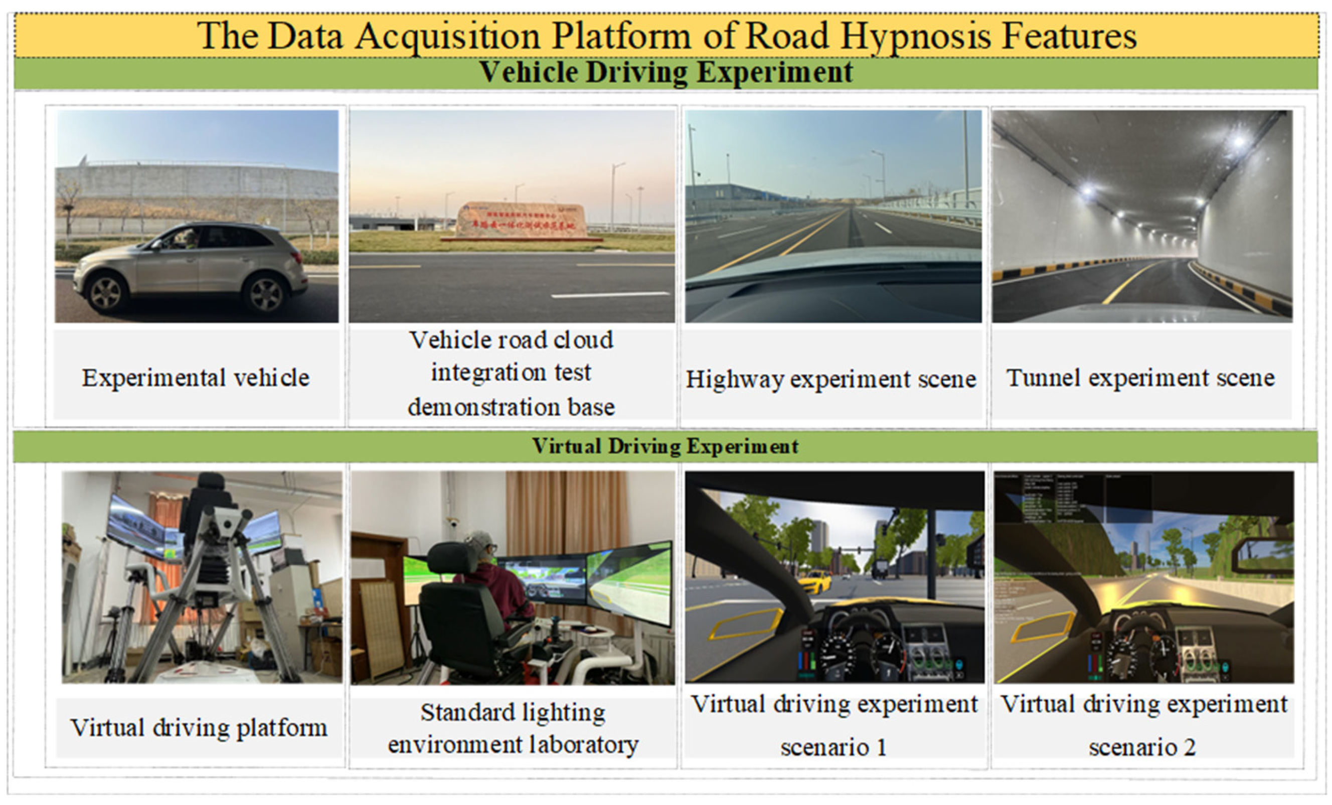
3.2. Experiment
3.2.1. Induction and Data Acquisition Methods of Road Hypnosis
- (1)
- In terms of the selection of drivers, drivers who are more prone to road hypnosis are selected for experiments in this study. Because novice drivers drive vehicles relatively seriously and are not prone to road hypnosis. Novice drivers may be nervous or serious while driving, which will affect the experimental results. In order to reduce or eliminate this effect, this study did not select novice drivers as research subjects. It is required that the driver has more than 8 years of driving experience. The driver is required to be between 26 and 60 years old, physically and mentally healthy, with relatively fixed sleep habits and sleeping time points. In order to avoid differences in results due to gender, all drivers recruited in this experiment are male. A total of 45 men are selected as drivers in the experiment
- (2)
- In terms of the selection of experimental scenarios, scenes with relatively simple road geometry need to be selected for the vehicle driving experiment and the virtual driving experiment. Based on previous research results [16], drivers’ road hypnosis is more likely to be induced by monotonous environments, such as tunnels and highways. This is because the design of highways usually pursues smoothness and high speed, so the road layout often lacks complex visual stimulation and changes. Due to the closure and unique light changes, tunnels can produce multiple sensory stimulations to the driver in a short period of time. These factors make it easier for drivers to be in a state of road hypnosis when driving in such an environment. Therefore, two scenarios, highway and tunnel, are selected to carry out the vehicle driving experiment and virtual driving experiment in this study.
- (3)
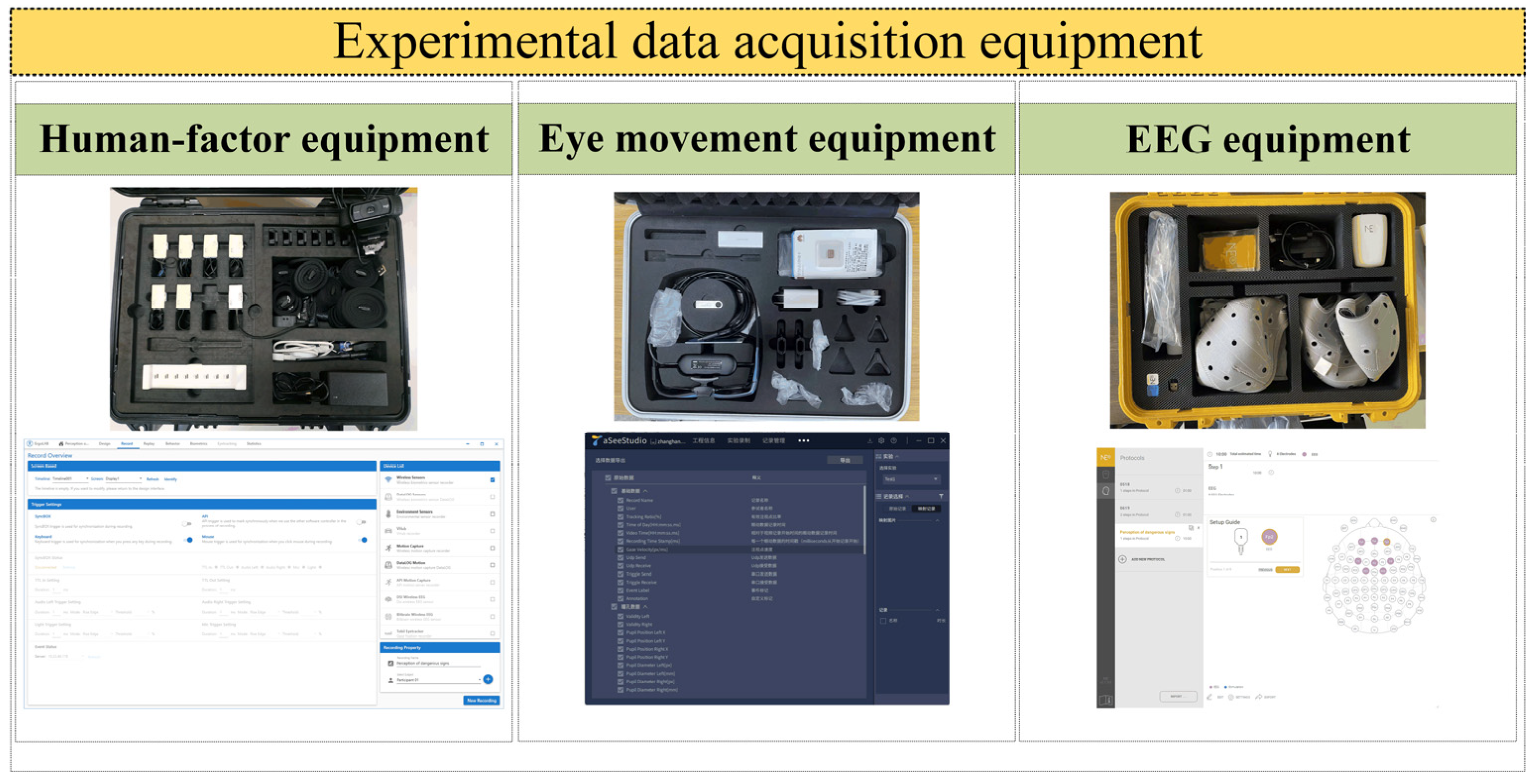
- In the process of vehicle driving and virtual driving experiments, the experimental assistant observes the subject’s eye movement, electroencephalogram, electrocardiogram, and other information collected by eye movement equipment, EEG equipment, and human-factor equipment in real time. The relevant data, when the driver’s eye movement gaze point is concentrated in the center of the road ahead, and the EEG, electrocardiogram, and electrocardiogram characteristics are stable, are recorded. The experimental assistant immediately asks whether the driver was just in a state of road hypnosis after the driver is out of this state, and records the response, so as to build a road hypnosis state driving data with such data. Because during the driving process, the road hypnosis state is presented as an intermittent and discontinuous multiple appearance, rather than a long-term stable and continuous state, the constructed road hypnotic state data set is stitched together from multiple time series data, not a long-term continuous data. At the same time, the conventional driving data in the non-road hypnosis state is selected as the normal driving data set.
- (4)
- After the data set is screened, the relevant researchers in the laboratory manually evaluate the selected data set and screen the collected data according to video playback. To organize and classify the experimental data, colleagues with relevant research experience in the laboratory utilize the recorded time points and periods from the experiment, and manually screen the ECG signals recorded during the experiment. The experimental data with typical road hypnosis characteristics is selected to make the road hypnosis data set. Compared to normal driving conditions, the gaze points of drivers in road hypnosis are more concentrated, the fixation durations are longer, and the blink durations increase in terms of eye movement characteristics. Compared to normal driving conditions, the heart rate variability of drivers is reduced, and the driver has a lower and more regular heart rate in terms of bioelectric characteristics. Similarly, the data with abnormal driving states is used to make the normal driving data set. During the experiment, individual subjects may be in a fatigued driving state due to physical consumption, irregular driving posture, and other factors. The data related to such situations will be eliminated. Finally, the road hypnosis data set and the normal driving data set are filtered out. The detailed method for determining the road hypnotic state can be found in reference [12].
3.2.2. Scenes and Equipment
3.2.3. The Procedure of Experiment
- (1)
- Vehicle driving experiment
- a.
- Before the experiment, an experimental assistant puts on eye movement equipment and the EEG equipment for the subjects and connects them to the laptop. At the beginning of the experiment, the experimental assistant is responsible for recording the start time and total duration of the experiment.
- b.
- The experiment begins at the specified time, and the subjects drive the vehicle from the starting point of the tunnel or highway to the end point. During this journey, an experimental assistant is responsible for observing the road conditions and ensuring the safety of the subjects. The other two experimental assistants are responsible for collecting the road hypnosis status data of the subjects. After reaching the finish line, subjects are required to rest for 15 min. During this period, the experimental assistants disassemble the equipment, debug the experimental equipment, check the power of the equipment, and collect other information. An experimental assistant takes the initiative to ask the subject if they felt a road hypnosis in the driving process and records it.
- c.
- Repeat the above experimental process. After all the experimenters collect the data, sort out the experimental equipment and end the experiment.
- (2)
- Virtual driving experiment
- a.
- Before the experiment, an experimental assistant is responsible for debugging the equipment and putting on the required equipment for the subjects. Subjects board the virtual driving platform. At the beginning of the experiment, the experimental assistant is responsible for recording the start time and overall duration of the experiment.
- b.
- In the experiment, subjects perform driving tasks as required. They are required to keep the vehicle speed at 120 km/h. They are not allowed to change lanes in the middle. They must turn back when driving to the end. During the experiment, two experimental assistants are responsible for collecting the road hypnosis status data of the subjects until the end of the virtual driving mission section.
- c.
- After a single experiment, an experimental assistant takes the initiative to ask the subject whether there are abnormal behaviors such as hypnosis and sleepiness during the driving process, records the subjects with abnormal behaviors, and asks whether the subjects are aware of entering road hypnosis, and records the answers. During this period, an experimental assistant is responsible for inspecting and debugging the equipment. The subjects exit the virtual driving platform. The experimental assistant helps the subjects take off the experimental equipment.
- d.
- The above experimental process is repeated until all subjects complete the experiment. After the experiment is completed, the experimental equipment is sorted, and the experiment ends.
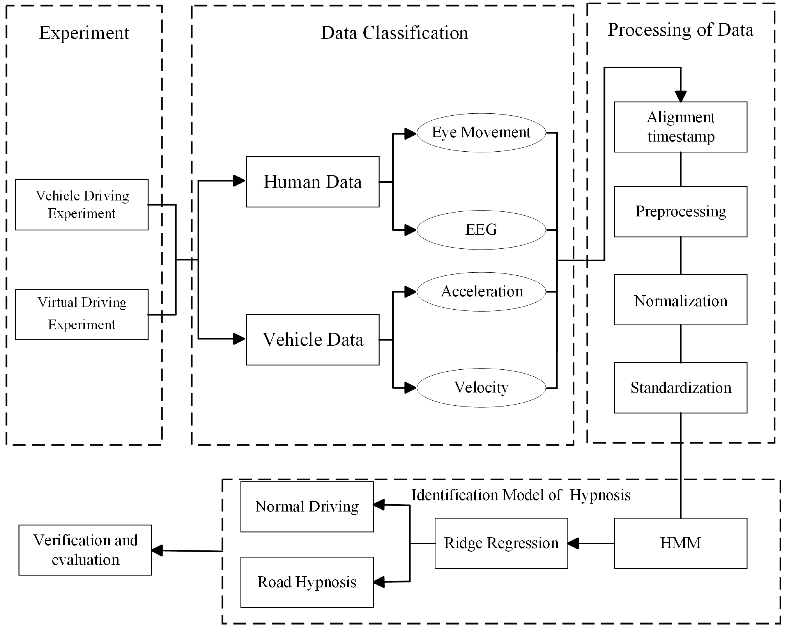
3.3. Model and Algorithms
3.3.1. Data Preprocessing Method
- (1)
- Original data types and data processing methods
- a.
- Data collection settings: The EEG data channels selected in this study are all located in the frontal lobe area. The Fp2, Fpz, Fp1, F4, Fz, F3, FC2, and FC1 channels are selected. The basis for selecting these channels is based on the previous research of the reference team [13]. The EEG sampling rate is set to 500 Hz. The sampling rate of eye movement data and vehicle data is set to 100 Hz. In order not to affect the data of each frequency band of EEG data, the EEG data filtering range in this study is 0.2 to 60 Hz.
- b.
- Data collation: After the data collection is completed, the EEG, eye movement data, and vehicle data obtained from vehicle driving and virtual driving experiments are sorted out. Forty groups of data are collected. EEG data are positioned by electrodes, bilateral mastoid average reference, filtering processing [24]. Eye movement data are initially screened and filtered [25], and vehicle data are filtered [26].
- c.
- EEG
- d.
- Eye movement data
- e.
- Vehicle data
- (2)
- Data normalization and standardization
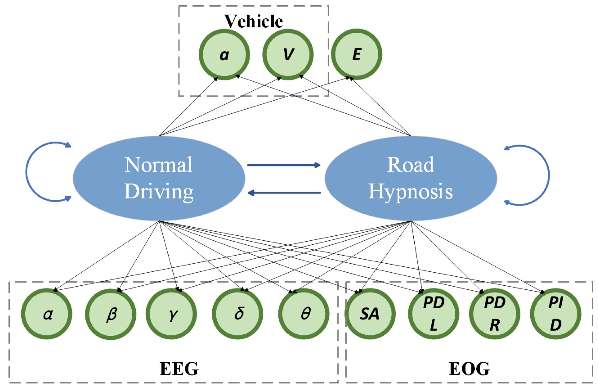
3.3.2. Road Hypnosis State Recognition Algorithm and Model
4. Extraction of Road Hypnosis State Characteristics
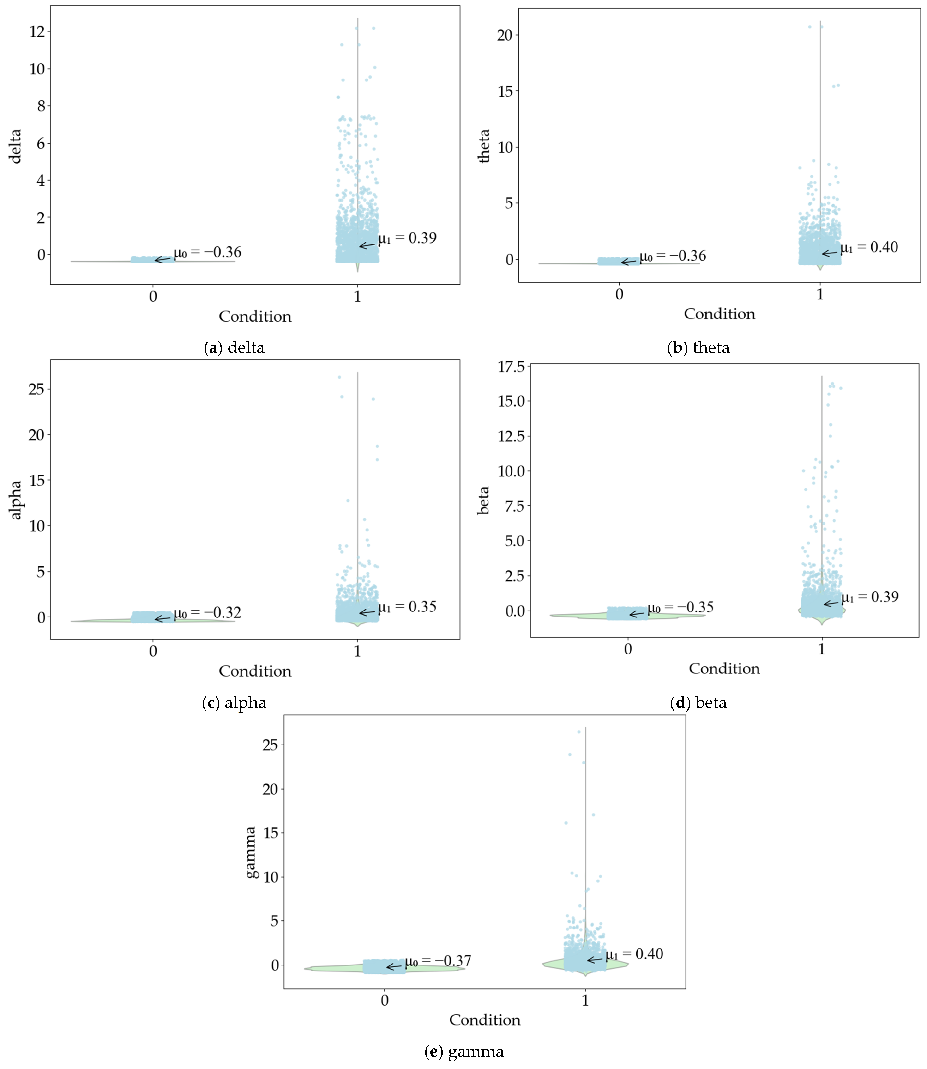
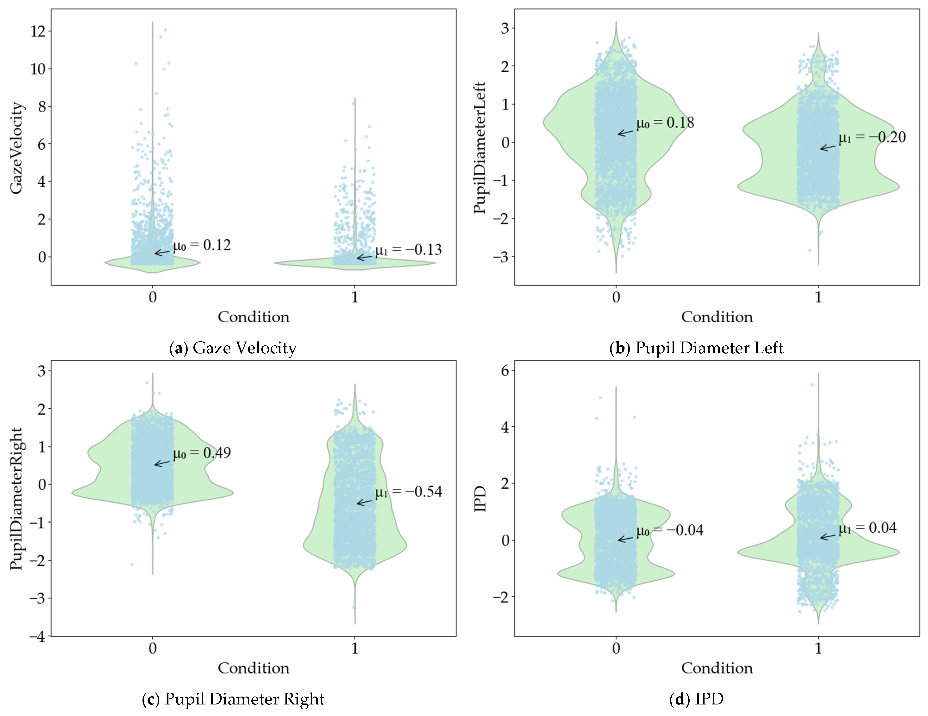
4.1. Human Characteristics of Drivers
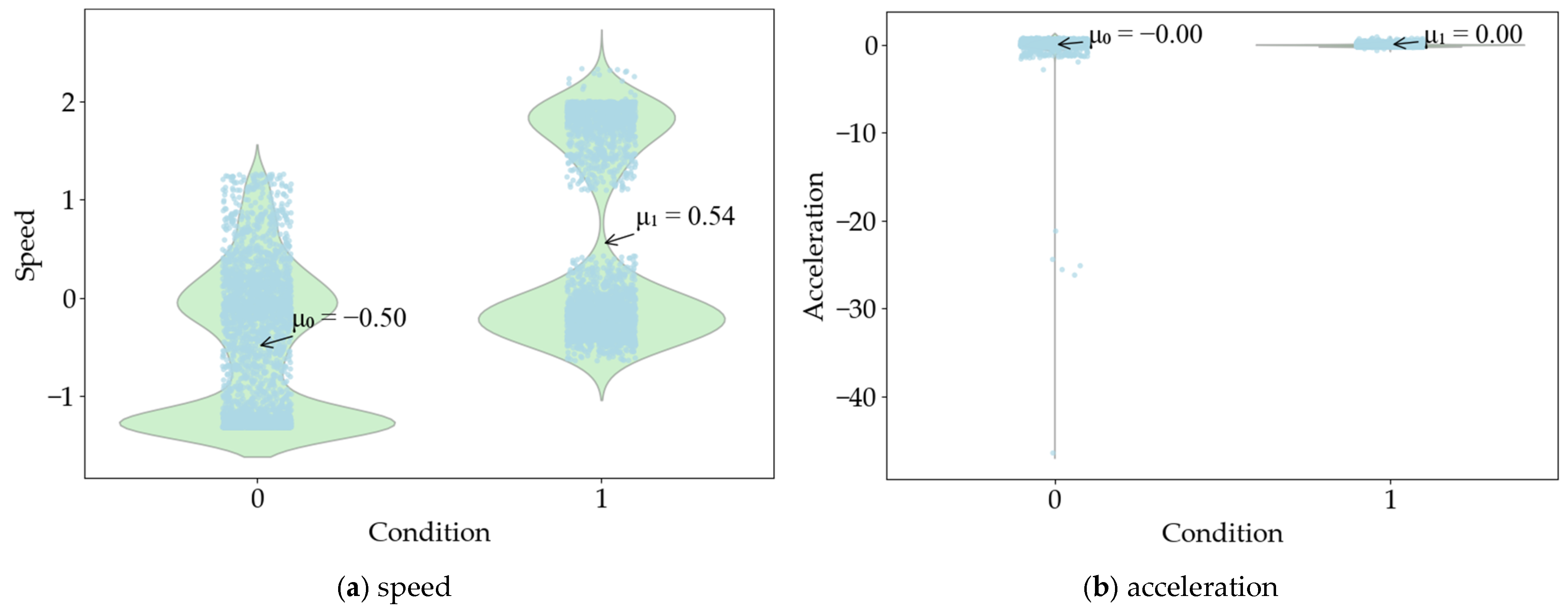
4.2. Vehicle Characteristics
5. Results and Analysis
6. Conclusions
- (1)
- Vehicle and virtual driving experiments are designed and conducted. Data from 45 participants in both road hypnosis and normal driving states were collected. A road hypnosis state characteristic data set is established, which lays the foundation for the preprocessing and analysis of road hypnosis characteristic parameters and the construction of the road hypnosis identification model.
- (2)
- Preprocessing methods for human data and vehicle data are introduced, which provide a cleaner and more standardized data basis for feature parameter extraction and model construction. The independent parameter t-test method is used to test the significance of driver characteristic data and vehicle characteristic data. Road hypnosis state characteristic parameters are extracted and used as input parameters for the subsequent road hypnosis identification model construction.
- (3)
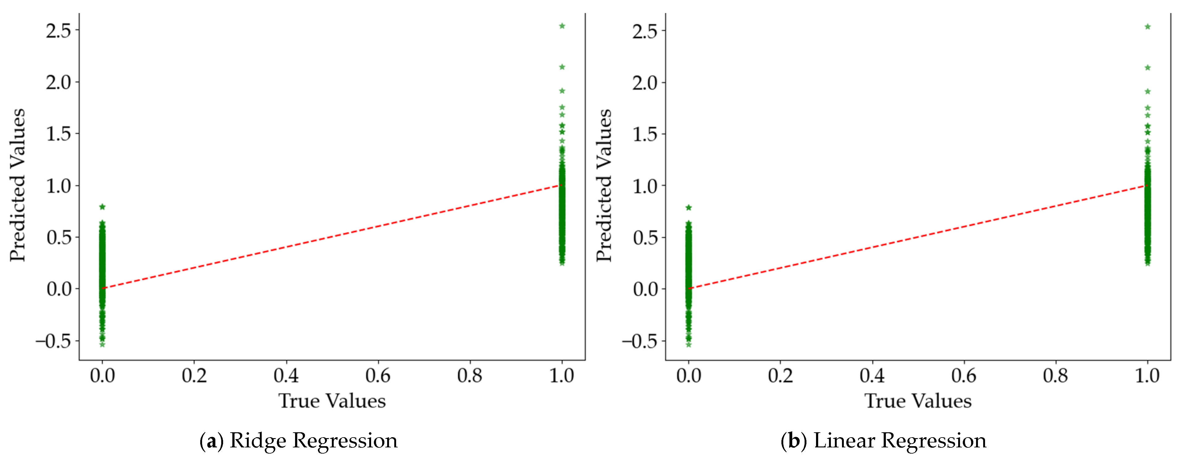
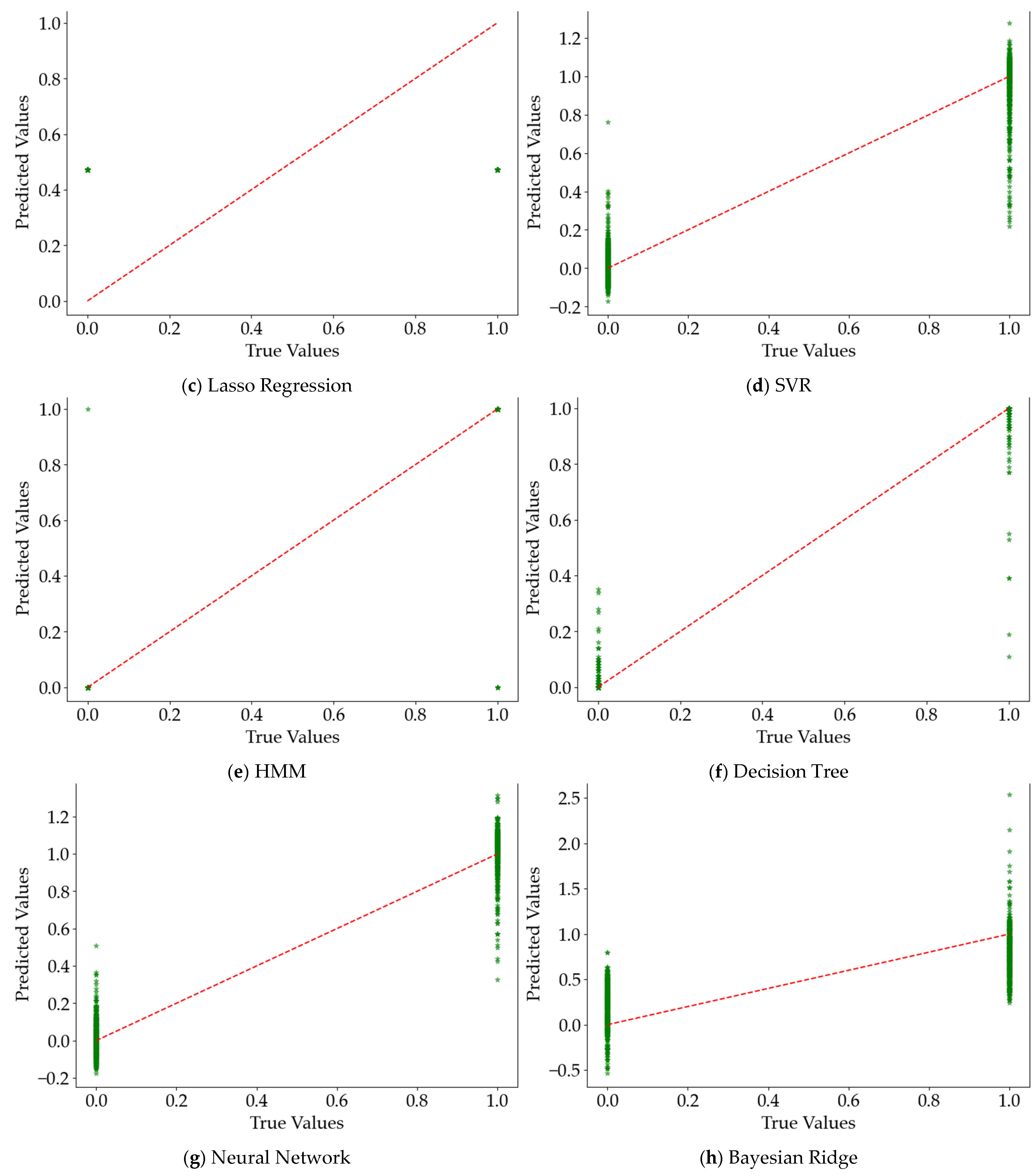
- A road hypnosis state identification model for car drivers based on Hidden Markov-Ridge Regression is constructed. To verify the effectiveness and accuracy of the model, it is compared and analyzed with regression models such as Linear Regression, Ridge Regression, Lasso Regression, Support Vector Regression (SVR), Decision Tree, Neural Network, and Bayesian Ridge Regression. Six evaluation metrics, including Mean Squared Error (MSE), Coefficient of Determination (R2), Root Mean Squared Error (RMSE), Mean Absolute Error (MAE), Explained Variance (EV), and Maximum Error, are introduced for model evaluation. The superiority of the constructed Hidden Markov-Ridge Regression model is verified.
Author Contributions
Funding
Institutional Review Board Statement
Informed Consent Statement
Data Availability Statement
Conflicts of Interest
References
- Miles, W. Sleeping with the eyes open. Sci. Am. 1929, 140, 489–492. [Google Scholar] [CrossRef]
- Sielski, M.C. Operational and Maintenance Problems on the Interstate System. 1959. Available online: https://docs.lib.purdue.edu/roadschool/1959/proceedings/10/ (accessed on 1 January 2025).
- Moseley, A. Hypnogogic hallucinations in relation to accidents. In Proceedings of the Trabajo Presentado en the American Psychological Association Convention, Cleveland, OH, USA, 4–9 September 1953. [Google Scholar]
- Lauer, A.R. The Psychology of Driving: Factors of Traffic Enforcement. 1960. Available online: https://archive.org/details/psychologyofdriv00lauerich/page/86/mode/2up (accessed on 24 April 2024).
- Hoskovec, J.; Svorad, D. Der Einflus der Monotonie des Reizfeldes auf Kraftfahrer. Verkehrsmedizan Und Ihre Grenzgeb. 1961, 8, 231–236. [Google Scholar]
- Khotimah, K. Analysis of Driver Fatigue Caused by Highway Hypnosis in Monotonous Geometrics of Road: State of the Arth Review. In Proceedings of the 9th International Conference on Civil Structural and Transportation Engineering (ICCSTE 2024) Chestnut Conference Centre, Toronto, ON, Canada, 13–15 June 2024. [Google Scholar] [CrossRef]
- Williams, G.W. Highway hypnosis: A hypothesis. Int. J. Clin. Exp. Hypn. 1963, 11, 143–151. [Google Scholar] [CrossRef] [PubMed]
- Williams, G.W.; Shor, R.E. An historical note on highway hypnosis. Accid. Anal. Prev. 1970, 2, 223–225. [Google Scholar] [CrossRef]
- Wertheim, A. Explaining highway hypnosis: Experimental evidence for the role of eye movements. Accid. Anal. Prev. 1978, 10, 111–129. [Google Scholar] [CrossRef]
- Cerezuela, G.P.; Tejero, P.; Chóliz, M.; Chisvert, M.; Monteagudo, M.J. Wertheim’s hypothesis on ‘highway hypnosis’: Empirical evidence from a study on motorway and conventional road driving. Accid. Anal. Prev. 2004, 36, 1045–1054. [Google Scholar] [CrossRef]
- Larue, G.S.; Rakotonirainy, A.; Pettitt, A.N. Driving performance impairments due to hypovigilance on monotonous roads. Accid. Anal. Prev. 2011, 43, 2037–2046. [Google Scholar] [CrossRef]
- Chen, L.; Wang, J.; Wang, X.; Wang, B.; Zhang, H.; Feng, K.; Wang, G.; Han, J.; Shi, H. A road hypnosis identification method for drivers based on fusion of biological characteristics. Digit. Transp. Saf. 2024, 3, 144–154. [Google Scholar] [CrossRef]
- Wang, B.; Wang, J.; Wang, X.; Chen, L.; Zhang, H.; Jiao, C.; Wang, G.; Feng, K. An identification method for road hypnosis based on human EEG data. Sensors 2024, 24, 4392. [Google Scholar] [CrossRef]
- Wang, B.; Wang, J.; Wang, X.; Chen, L.; Jiao, C.; Zhang, H.; Liu, Y. An Identification Method for Road Hypnosis Based on the Fusion of Human Life Parameters. Sensors 2024, 24, 7529. [Google Scholar] [CrossRef]
- Zhou, S.; Zhang, N.; Duan, Q.; Liu, X.; Xiao, J.; Wang, L.; Yang, J. Monitoring and Analyzing Driver Physiological States Based on Automotive Electronic Identification and Multimodal Biometric Recognition Methods. Algorithms 2024, 17, 547. [Google Scholar] [CrossRef]
- Sun, L.; Yang, H.; Li, B. Multimodal Dataset Construction and Validation for Driving-Related Anger: A Wearable Physiological Conduction and Vehicle Driving Data Approach. Electronics 2024, 13, 3904. [Google Scholar] [CrossRef]
- Xiang, G.; Yao, S.; Deng, H.; Wu, X.; Wang, X.; Xu, Q.; Yu, T.; Wang, K.; Peng, Y. A multi-modal driver emotion dataset and study: Including facial expressions and synchronized physiological signals. Eng. Appl. Artif. Intell. 2024, 130. [Google Scholar] [CrossRef]
- Park, S.; You, J. Development of Driver State Monitoring System based on Multi-Sensor Data Fusion. Preprints 2023. [Google Scholar] [CrossRef]
- Tan, D.; Tian, W.; Wang, C.; Chen, L.; Xiong, L. Driver Distraction Behavior Recognition for Autonomous Driving: Approaches, Datasets and Challenges. IEEE Trans. Intell. Veh. 2024. [Google Scholar] [CrossRef]
- Qu, Y.; Hu, H.; Liu, J.; Zhang, Z.; Li, Y.; Ge, X. Driver state monitoring technology for conditionally automated vehicles: Review and future prospects. IEEE Trans. Instrum. Meas. 2023, 72, 3000920. [Google Scholar] [CrossRef]
- Wang, L.; Song, F.; Zhou, T.H.; Hao, J.; Ryu, K.H. EEG and ECG-based multi-sensor fusion computing for real-time fatigue driving recognition based on feedback mechanism. Sensors 2023, 23, 8386. [Google Scholar] [CrossRef]
- Eddy, S.R. Hidden markov models. Curr. Opin. Struct. Biol. 1996, 6, 361–365. [Google Scholar] [CrossRef]
- Sotoodeh, M.; Ho, J.C. Improving length of stay prediction using a hidden Markov model. AMIA Summits Transl. Sci. Proc. 2019, 2019, 425. [Google Scholar]
- Chaddad, A.; Wu, Y.; Kateb, R.; Bouridane, A. Electroencephalography signal processing: A comprehensive review and analysis of methods and techniques. Sensors 2023, 23, 6434. [Google Scholar] [CrossRef]
- Landes, J.; Köppl, S.; Klettke, M. Data Processing Pipeline for Eye-Tracking Analysis. In Proceedings of the 35th GI-Workshop on Foundations of Databases (Grundlagen von Datenbanken), Herdecke, Germany, 22–24 May 2024. [Google Scholar]
- Kumar, S.V. Traffic flow prediction using Kalman filtering technique. Procedia Eng. 2017, 187, 582–587. [Google Scholar] [CrossRef]
- Shakil, S.; Lee, C.-H.; Keilholz, S.D. Evaluation of sliding window correlation performance for characterizing dynamic functional connectivity and brain states. Neuroimage 2016, 133, 111–128. [Google Scholar] [CrossRef] [PubMed]
- Bertocci, U.; Frydman, J.; Gabrielli, C.; Huet, F.; Keddam, M. Analysis of electrochemical noise by power spectral density applied to corrosion studies: Maximum entropy method or fast Fourier transform? J. Electrochem. Soc. 1998, 145, 2780. [Google Scholar] [CrossRef]
- Wang, X.; Chen, L.; Shi, H.; Han, J.; Wang, G.; Wang, Q.; Zhong, F.; Li, H. A real-time recognition system of driving propensity based on AutoNavi navigation data. Sensors 2022, 22, 4883. [Google Scholar] [CrossRef] [PubMed]
- Cabello-Solorzano, K.; Ortigosa de Araujo, I.; Peña, M.; Correia, L.J.; Tallón-Ballesteros, A. The impact of data normalization on the accuracy of machine learning algorithms: A comparative analysis. In Proceedings of the International Conference on Soft Computing Models in Industrial and Environmental Applications, Salamanca, Spain, 5–7 September 2023; Springer Nature: Cham, Switzerland, 2023; pp. 344–353. [Google Scholar] [CrossRef]
- Gal, M.S.; Rubinfeld, D.L. Data standardization. NYUL Rev. 2019, 94, 737. [Google Scholar] [CrossRef]
- Kim, T.K. T test as a parametric statistic. Korean J. Anesthesiol. 2015, 68, 540–546. [Google Scholar] [CrossRef]
- Chicco, D.; Warrens, M.J.; Jurman, G. The coefficient of determination R-squared is more informative than SMAPE, MAE, MAPE, MSE and RMSE in regression analysis evaluation. Peerj Comput. Sci. 2021, 7, e623. [Google Scholar] [CrossRef]
- Su, X.; Yan, X.; Tsai, C.L. Linear regression. Wiley Interdiscip. Rev. Comput. Stat. 2012, 4, 275–294. [Google Scholar] [CrossRef]
- Ranstam, J.; Cook, J.A. LASSO regression. J. Br. Surg. 2018, 105, 1348. [Google Scholar] [CrossRef]
- Awad, M.; Khanna, R.; Awad, M.; Khanna, R. Support Vector Regression. Efficient Learning Machines: Theories, Concepts, and Applications for Engineers and System Designers; Apress: New York, NY, USA, 2015; pp. 67–80. [Google Scholar] [CrossRef]
- Song, Y.-Y.; Ying, L. Decision tree methods: Applications for classification and prediction. Shanghai Arch. Psychiatry 2015, 27, 130. [Google Scholar]
- Wu, Y.-C.; Feng, J.-W. Development and application of artificial neural network. Wirel. Pers. Commun. 2018, 102, 1645–1656. [Google Scholar] [CrossRef]
- Shi, Q.; Abdel-Aty, M.; Lee, J. A Bayesian ridge regression analysis of congestion’s impact on urban expressway safety. Accid. Anal. Prev. 2016, 88, 124–137. [Google Scholar] [CrossRef] [PubMed]
- Ethical Review Measures for Biomedical Research Involving Humans. Available online: https://www.gov.cn/zhengce/zhengceku/2023-02/28/content_5743658.htm (accessed on 18 February 2023).

| Type | Name | Explanation |
|---|---|---|
| Pupil information | Validity Left | Validity of left eye pupil recognition: 0 means the recognition is successful; 1 means the recognition fails |
| Validity Right | Validity of right eye pupil recognition: 0 means the recognition is successful; 1 means the recognition fails | |
| Pupil Diameter Left (mm) | Left eye pupil diameter | |
| Pupil Diameter Right (mm) | Right eye pupil diameter | |
| IPD (mm) | Interpupillary distance | |
| Gaze point information | Gaze Point Index | Original gaze point index |
| Gaze Velocity(px/s) | The speed at which the eyes move | |
| Gaze Point X (px) | Original fixation x-coordinate in pixels | |
| Gaze Point Y (px) | Original fixation y-coordinate in pixels | |
| Gaze Point Right X (px) | X-coordinate of the original gaze point of the right eye | |
| Gaze Point Right Y (px) | Y-coordinate of the original gaze point of the right eye | |
| Gaze Point Left X (px) | X-coordinate of the original gaze point of the left eye | |
| Gaze Point Left Y (px) | Y-coordinate of the original gaze point of the left eye | |
| Gaze Vector Left X | The x-coordinate of the left eye gaze vector | |
| Gaze Vector Left Y | The y-coordinate of the left eye gaze vector | |
| Gaze Vector Left Z | The z-coordinate of the left eye gaze vector | |
| Gaze Vector Right X | The x-coordinate of the right eye gaze vector | |
| Gaze Vector Right Y | The y-coordinate of the right eye gaze vector | |
| Gaze Vector Right Z | The z-coordinate of the left eye gaze vector |
| Observation Sequence | Regression Coefficient | Observation Sequence | Regression Coefficient |
|---|---|---|---|
| Speed | β1 | gamma | β8 |
| Acceleration | β2 | Gaze Velocity | β9 |
| Delta | β4 | Pupil Diameter Left | β10 |
| Theta | β5 | Pupil Diameter Right | β12 |
| Alpha | β6 | IPD | β14 |
| Beta | β7 | Intercept | β0 |
| Levin’s Variance Equivariance Test | Mean Equivalence t Test | |||||||
|---|---|---|---|---|---|---|---|---|
| F | Significance | t | Degree of Freedom | Sig. (2-Tailed) | Average Deviation | Standard Error | ||
| delta | Homoscedasticity assumption | 1908.694 | 0.000 | 30.090 | 5538 | 0.000 | 0.751 | 0.025 |
| Heteroscedasticity assumption | 28.711 | 2642.050 | 0.000 ** | 0.751 | 0.026 | |||
| theta | Homoscedasticity assumption | 1806.138 | 0.000 | 30.438 | 5538 | 0.000 | 0.758 | 0.025 |
| Heteroscedasticity assumption | 29.051 | 2656.262 | 0.000 ** | 0.758 | 0.026 | |||
| alpha | Homoscedasticity assumption | 446.060 | 0.000 | 26.033 | 5538 | 0.000 | 0.661 | 0.025 |
| Heteroscedasticity assumption | 24.885 | 2736.688 | 0.000 ** | 0.661 | 0.027 | |||
| beta | Homoscedasticity assumption | 486.039 | 0.000 | 29.443 | 5538 | 0.000 | 0.737 | 0.025 |
| Heteroscedasticity assumption | 28.124 | 2698.158 | 0.000 ** | 0.737 | 0.026 | |||
| gamma | Homoscedasticity assumption | 307.435 | 0.000 | 30.904 | 5538 | 0.000 | 0.768 | 0.025 |
| Heteroscedasticity assumption | 29.621 | 2884.348 | 0.000 ** | 0.768 | 0.026 | |||
| Levin’s Variance Equivariance Test | Mean Equivalence t Test | |||||||
|---|---|---|---|---|---|---|---|---|
| F | Significance | t | Degree of Freedom | Sig. (2-Tailed) | Average Deviation | Standard Error | ||
| Gaze Velocity | Homoscedasticity assumption | 192.138 | 0.000 | −9.548 | 5538 | 0.000 | −0.255 | 0.027 |
| Heteroscedasticity assumption | −9.722 | 5090.659 | 0.000 ** | −0.255 | 0.026 | |||
| Pupil Diameter Right | Homoscedasticity assumption | 796.958 | 0.000 | −44.350 | 5538 | 0.000 | −1.025 | 0.023 |
| Heteroscedasticity assumption | −43.440 | 4336.223 | 0.000 ** | −1.025 | 0.024 | |||
| Pupil Diameter Left | Homoscedasticity assumption | 54.213 | 0.000 | −14.514 | 5538 | 0.000 | −0.383 | 0.026 |
| Heteroscedasticity assumption | −14.631 | 5504.434 | 0.000 ** | −0.383 | 0.026 | |||
| IPD | Homoscedasticity assumption | 1.791 | 0.181 | 2.898 | 5538 | 0.004 ** | 0.078 | 0.027 |
| Heteroscedasticity assumption | 2.889 | 5401.695 | 0.004 | 0.078 | 0.027 | |||
| Levin’s Variance Equivariance Test | Mean Equivalence t Test | |||||||
|---|---|---|---|---|---|---|---|---|
| F | Significance | t | Degree of Freedom | Sig. (2-Tailed) | Average Deviation | Standard Error | ||
| Speed | Homoscedasticity assumption | 820.174 | 0.000 | 45.241 | 5538 | 0.000 | 1.040 | 0.0230 |
| Heteroscedasticity assumption | 44.698 | 4940.143 | 0.000 ** | 1.040 | 0.0233 | |||
| Acceleration | Homoscedasticity assumption | 29.406 | 0.000 | 0.306 | 5538 | 0.760 | 8.230 × 10⁻³ | 2.690 × 10⁻² |
| Heteroscedasticity assumption | 0.320 | 2989.189 | 0.749 | 8.230 × 10⁻³ | 2.570 × 10⁻² | |||
| Observation Sequence | Regression Coefficient | Value | Observation Sequence | Regression Coefficient | Value |
|---|---|---|---|---|---|
| Speed | β1 | 0.111 | Gaze Velocity | β9 | −0.017 |
| Delta | β4 | 0.097 | Pupil Diameter Left | β10 | 0.093 |
| Theta | β5 | 0.094 | Pupil Diameter Right | β12 | −0.235 |
| Alpha | β6 | 0.033 | IPD | β14 | 0.060 |
| Beta | β7 | −0.066 | Acceleration | β15 | 0.105 |
| Gamma | β8 | 0.089 | Intercept | β0 | 0.349 |
| Model | MSE | RMSE | MAE | R2 | EV | Max Error |
|---|---|---|---|---|---|---|
| Linear Regression | 0.100152 | 0.316469 | 0.257835 | 0.599232 | 0.59937 | 1.538337 |
| Ridge Regression | 0.100165 | 0.316488 | 0.257841 | 0.599184 | 0.599321 | 1.53835 |
| Lasso Regression | 0.250188 | 0.500188 | 0.499467 | −0.00115 | 0 | 0.52685 |
| SVR | 0.019759 | 0.140565 | 0.088761 | 0.920935 | 0.922042 | 0.78287 |
| Decision Tree | 0.004513 | 0.067176 | 0.004513 | 0.981942 | 0.981946 | 1 |
| HMM- Ridge Regression | 0.003068 | 0.055387 | 0.010866 | 0.987724 | 0.987748 | 0.89 |
| Neural Network | 0.009819 | 0.099092 | 0.065211 | 0.960707 | 0.960733 | 0.701525 |
| Bayesian Ridge | 0.100244 | 0.316614 | 0.2579 | 0.598865 | 0.599006 | 1.537624 |
Disclaimer/Publisher’s Note: The statements, opinions and data contained in all publications are solely those of the individual author(s) and contributor(s) and not of MDPI and/or the editor(s). MDPI and/or the editor(s) disclaim responsibility for any injury to people or property resulting from any ideas, methods, instructions or products referred to in the content. |
© 2025 by the authors. Licensee MDPI, Basel, Switzerland. This article is an open access article distributed under the terms and conditions of the Creative Commons Attribution (CC BY) license (https://creativecommons.org/licenses/by/4.0/).
Share and Cite
Zhang, H.; Chen, L.; Wang, B.; Wang, X.; Wang, J.; Jiao, C.; Feng, K.; Shen, C.; Wang, Q.; Han, J.; et al. Research on the Identification of Road Hypnosis Based on the Fusion Calculation of Dynamic Human–Vehicle Data. Sensors 2025, 25, 2846. https://doi.org/10.3390/s25092846
Zhang H, Chen L, Wang B, Wang X, Wang J, Jiao C, Feng K, Shen C, Wang Q, Han J, et al. Research on the Identification of Road Hypnosis Based on the Fusion Calculation of Dynamic Human–Vehicle Data. Sensors. 2025; 25(9):2846. https://doi.org/10.3390/s25092846
Chicago/Turabian StyleZhang, Han, Longfei Chen, Bin Wang, Xiaoyuan Wang, Jingheng Wang, Chenyang Jiao, Kai Feng, Cheng Shen, Quanzheng Wang, Junyan Han, and et al. 2025. "Research on the Identification of Road Hypnosis Based on the Fusion Calculation of Dynamic Human–Vehicle Data" Sensors 25, no. 9: 2846. https://doi.org/10.3390/s25092846
APA StyleZhang, H., Chen, L., Wang, B., Wang, X., Wang, J., Jiao, C., Feng, K., Shen, C., Wang, Q., Han, J., & Liu, Y. (2025). Research on the Identification of Road Hypnosis Based on the Fusion Calculation of Dynamic Human–Vehicle Data. Sensors, 25(9), 2846. https://doi.org/10.3390/s25092846