
Path Planning in Narrow Road Scenarios Based on Four-Layer Network Cost Structure Map
Abstract
1. Introduction
2. Materials and Methods
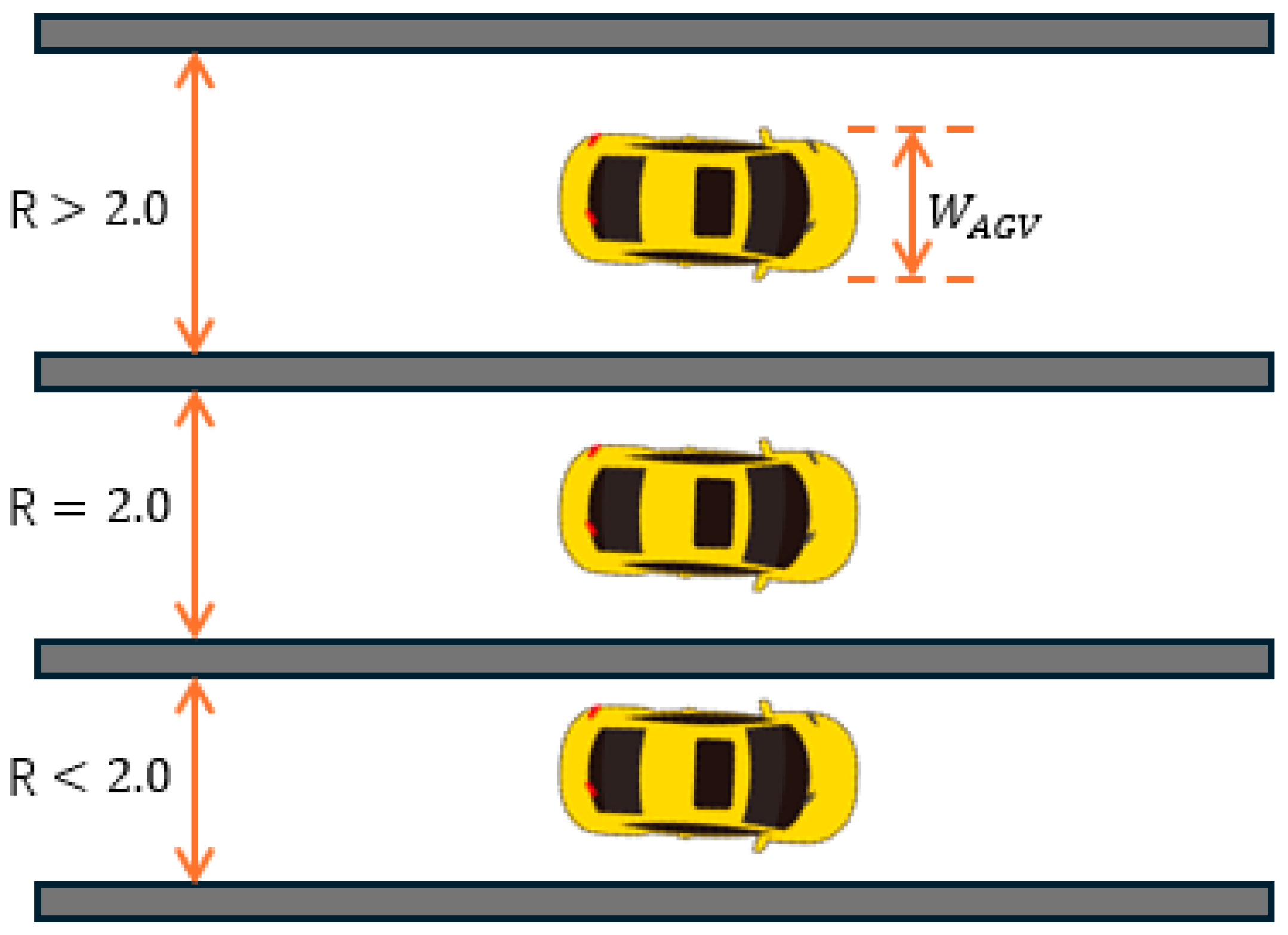
2.1. Definition for Narrow Road Scenarios
2.2. Voronoi Skeleton Description
2.3. New Cost Map of Four-Layer Network Structure
- (1)
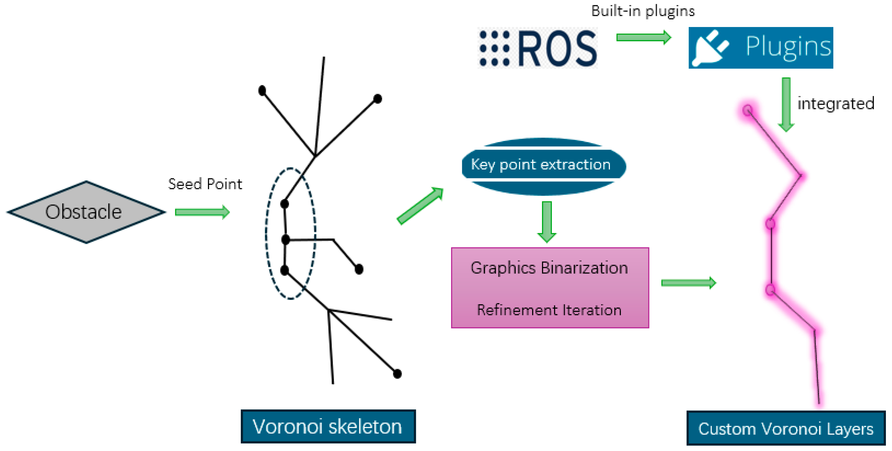
- Generation of Voronoi Diagram: First, the Voronoi algorithm is used to generate the Voronoi diagram of the entire environment. In this process, we regard the static obstacles in the environment as seed points and divide these obstacles into multiple Voronoi regions through the Voronoi diagram. Each Voronoi region represents the shortest distance from any point in the region to the nearest obstacle, and the boundary of the region is the dividing line between the obstacle and the free space.
- (2)
- Image Binarization: After generating the Voronoi diagram, we convert each region in the diagram into a binary image. In this binary image, the obstacle location and the Voronoi skeleton are marked as “1”, while other regions are marked as “0”. This step simplifies the Voronoi diagram into a binary form, which is convenient for subsequent skeleton extraction and refinement.
- (3)
- Voronoi skeleton refinement: The thinning algorithm is applied to the binary image to extract the core structure of the Voronoi skeleton. The thinning process iteratively removes unimportant boundary points and retains only the most important paths connected to the core of the region. At each iteration, the algorithm removes isolated points or redundant line segments in the image, and the final retained path is the Voronoi skeleton. The skeleton consists of several line segments connecting obstacles and free space, showing the influence range of obstacles in the environment.
- (4)
- Extract key points: In the refined Voronoi skeleton, we extract key points, which represent the main structure of the skeleton and the bifurcation points of the path. The extracted key points are usually located at the intersection of the boundary between obstacles and free space, or at the location where the path direction changes greatly in the skeleton. These key points will be used as constraints in path planning to ensure that the AGV path avoids obstacles and provides a safe distance.
- (5)
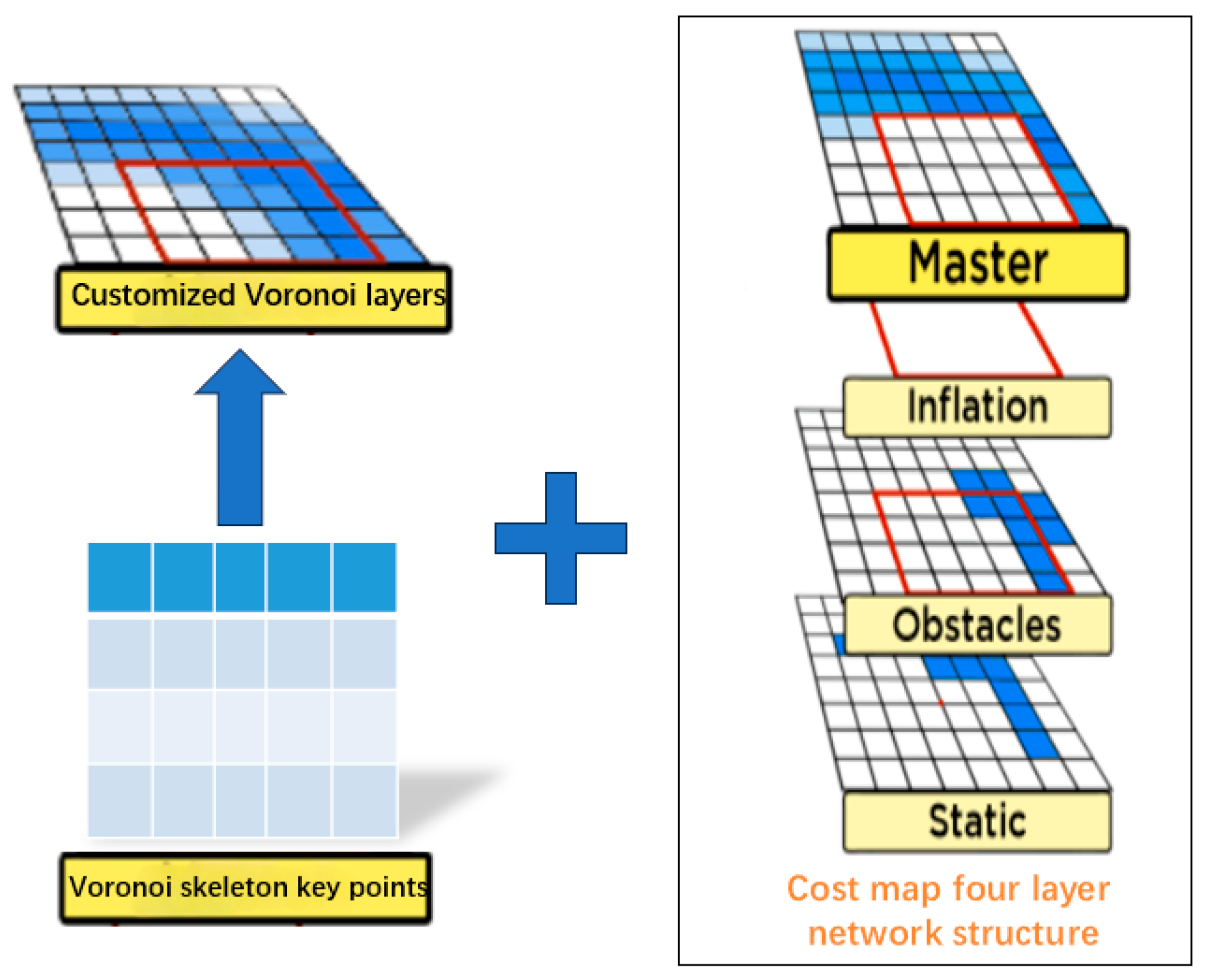
- Generate custom Voronoi layers: Through the extracted key points, we generated a custom Voronoi layer. This layer is used to represent the impact area and safety distance of obstacles from the perspective of AGV path planning. The custom Voronoi layer is combined with the traditional cost map (including static layer, obstacle layer and expansion layer) to form a new four-layer network structure.
- (6)
- Integration in ROS system: The generated Voronoi diagram data are integrated into the system through the plugin mechanism in the ROS system. Specifically, the plugin is responsible for receiving the generated Voronoi diagram data and converting it into a layer that can be used for AGV navigation. The custom Voronoi layer is combined with the traditional cost map to form a four-layer network structure, including static layer, obstacle layer, inflation layer, Voronoi layer. In this way, the cost map of the four-layer network structure can more accurately reflect the impact range of obstacles and improve the safety and efficiency of path planning.
2.4. Global Path Planning Based on New Cost Map
- (1)
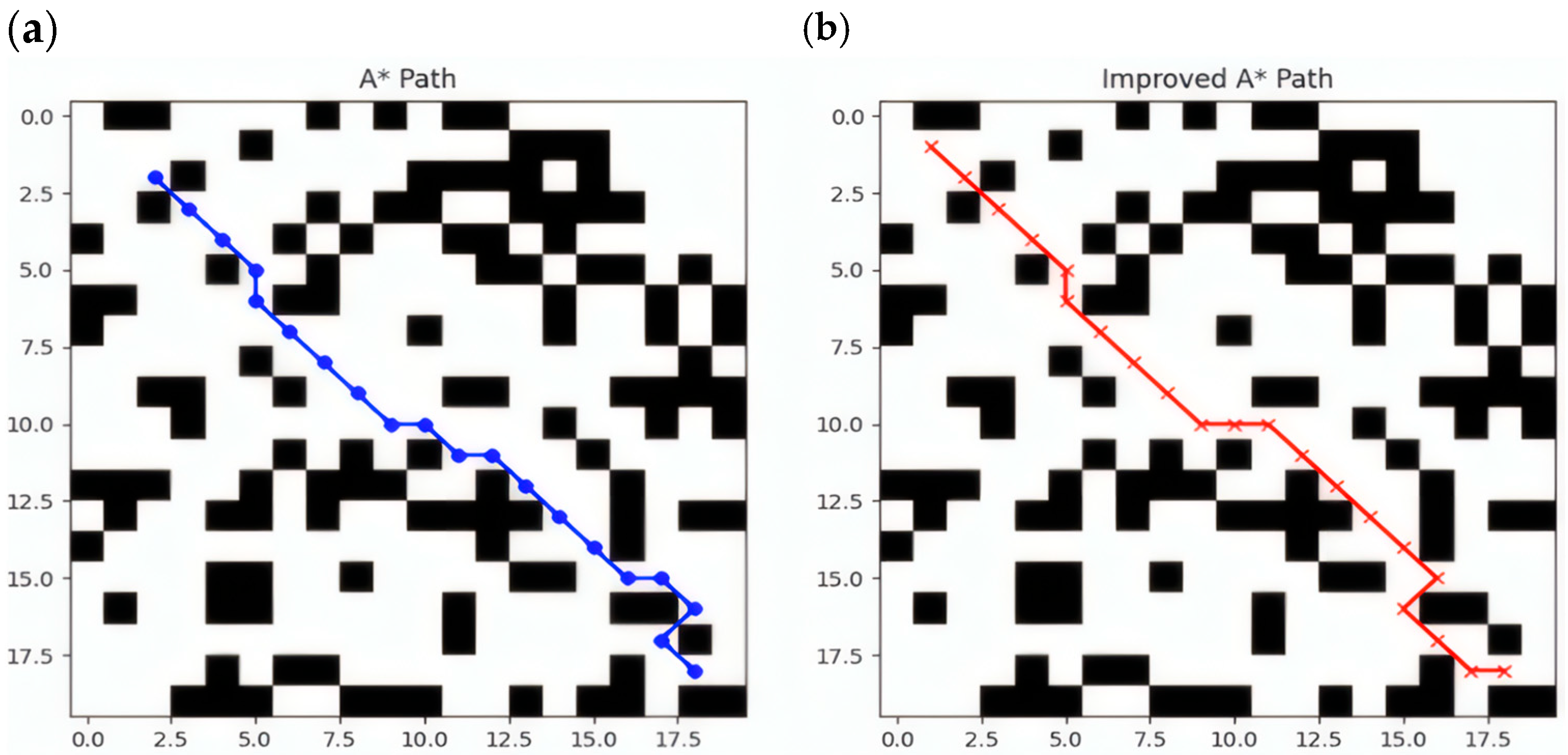
- Setting the grid map size: The grid map used in this experiment is 20 × 20, that is, a two-dimensional matrix with 20 rows and 20 columns, where each cell represents a grid.
- (2)
- Obstacle setting: In path planning algorithms, obstacles are usually generated by random number generators. To ensure that a consistent obstacle layout is generated in each experiment, we use a random seed to fix the starting state of the random number generator. This experimental map is simulated in Python3.9, and the random seed in the map is set by calling the built-in seed function. In this way, the generated random number sequence is the same each time it is run, ensuring the repeatability of the obstacle layout. In this study, obstacles are randomly distributed on the map with a probability of 40%. Specifically, each grid cell has a 40% probability of becoming an obstacle, and the rest is empty space. To achieve this, we generate a random number between 0 and 1 for each grid cell. If the random number is less than or equal to the set obstacle probability, the grid cell will be marked as an obstacle; otherwise, it will be a feasible path. In this way, we can simulate an environment with random obstacles for path planning algorithms to test and optimize.
- (3)
- Start and end point settings: The starting point is set at the upper left corner of the grid (coordinate (1, 1)); The end point is set near the lower right corner of the grid (coordinates (18, 18)), that is, a certain distance from the lower right corner.
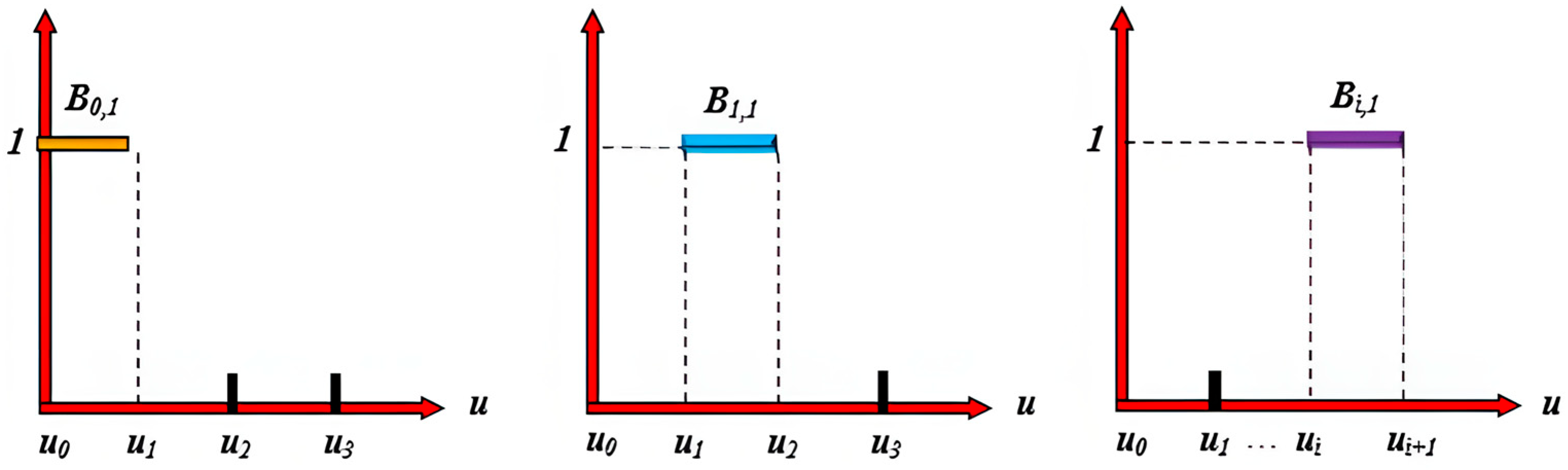
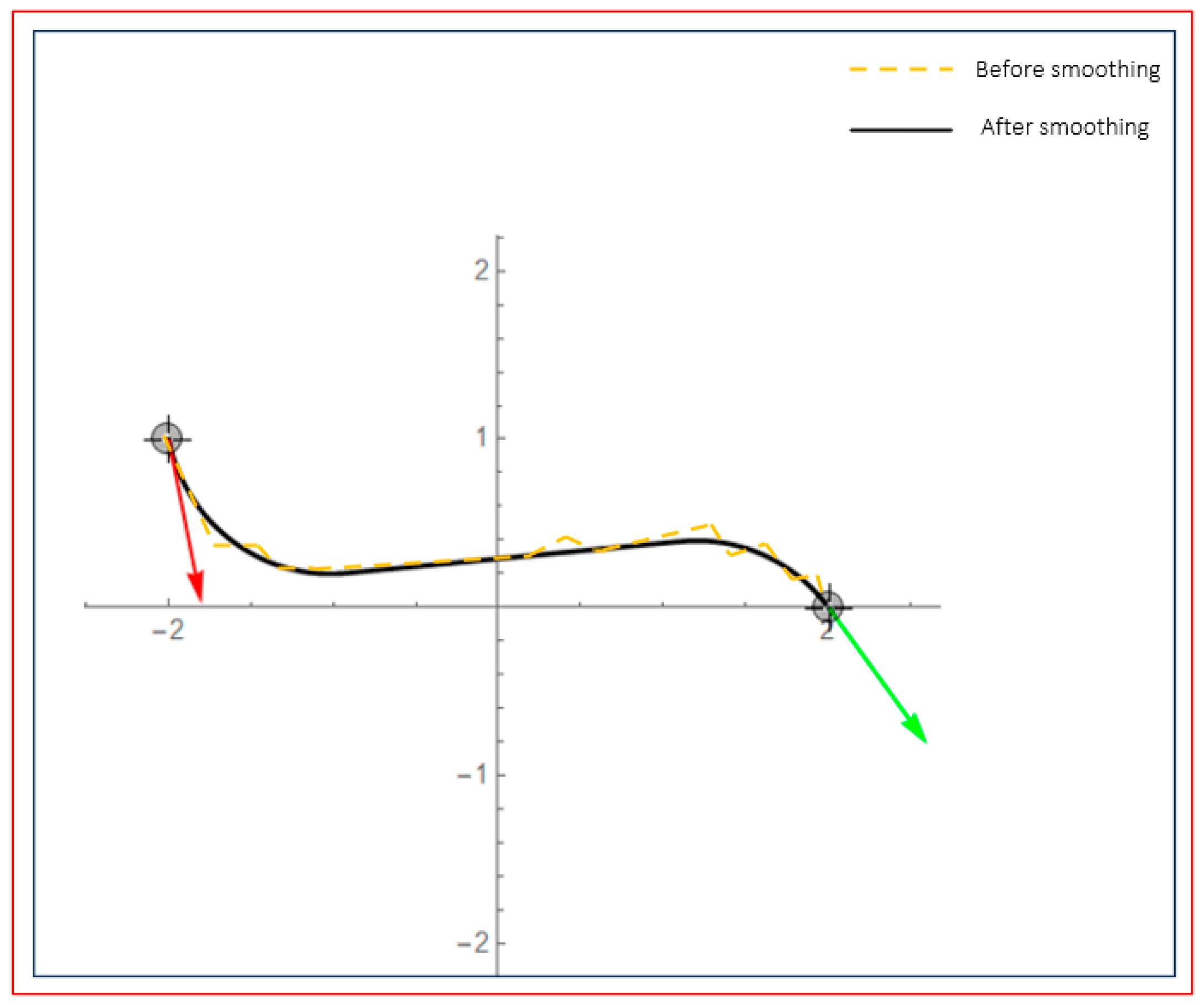
2.5. B-Spline Smoothing Optimization of Global Path
3. Results and Discussion
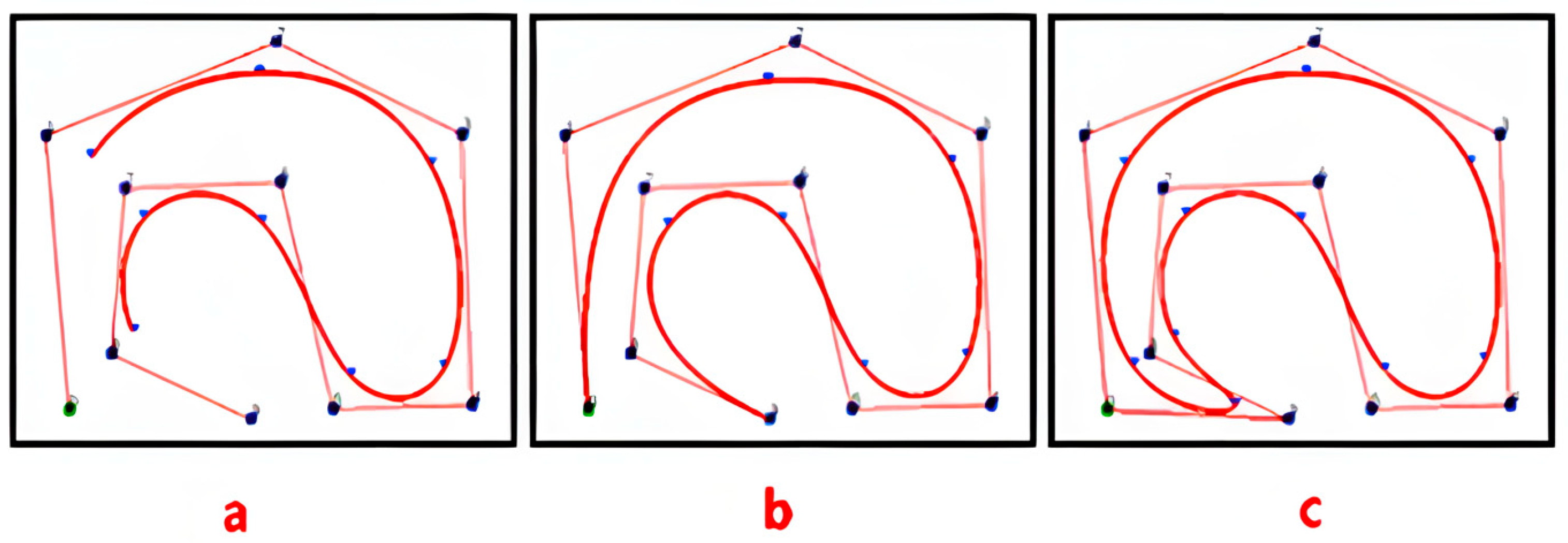
3.1. Verify the Security of the Algorithm in a Simulated Environment
3.2. Analysis of the Time and Space Complexity of This Algorithm
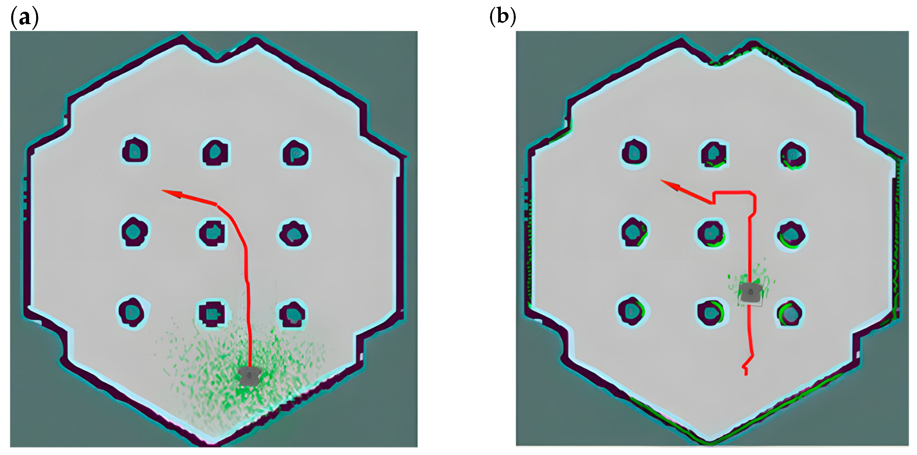
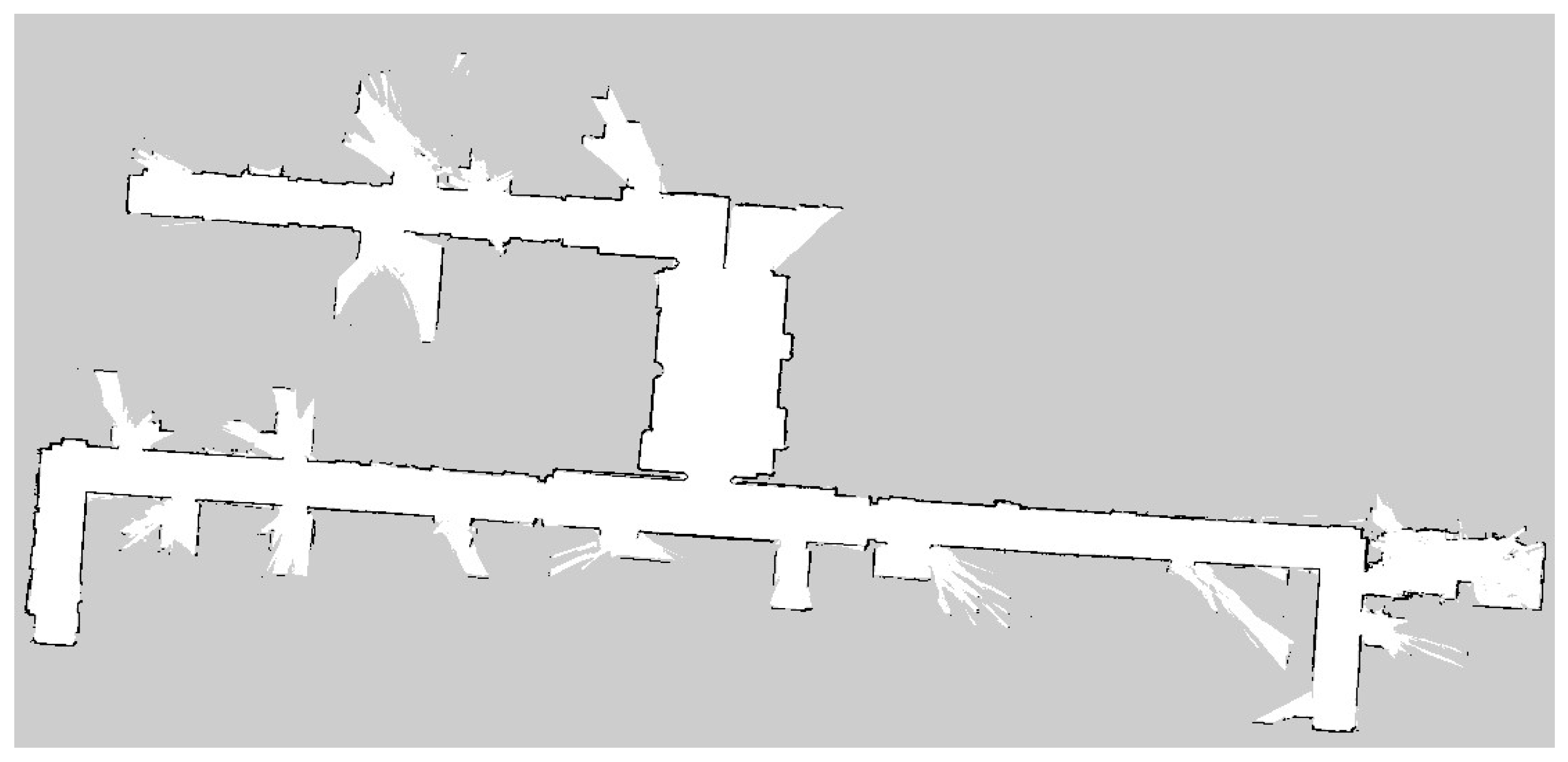
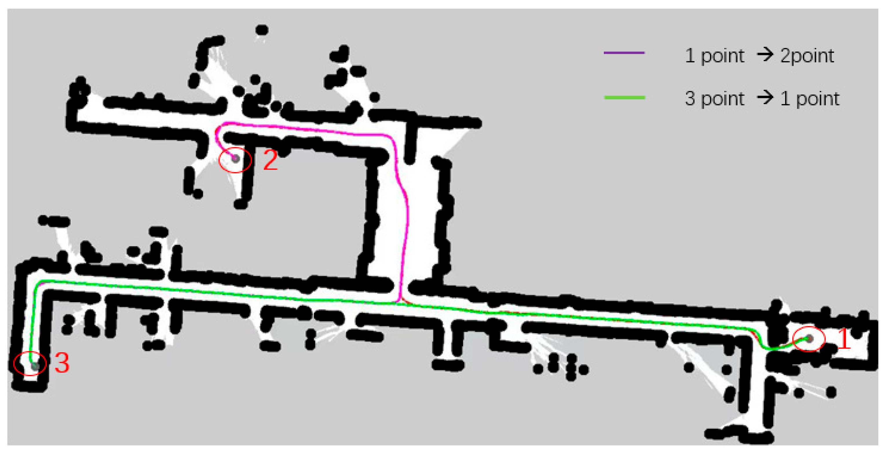
3.3. Experimental Verification and Analysis of Real Scenarios
4. Conclusions
Author Contributions
Funding
Institutional Review Board Statement
Informed Consent Statement
Data Availability Statement
Acknowledgments
Conflicts of Interest
References
- Tao, Y.; Duan, L.; Gao, H.; Zhang, Y.; Song, Y.; Wang, T. Heuristic Expanding Disconnected Graph: A Rapid Path Planning Method for Mobile Robots. Chin. J. Mech. Eng. 2024, 37, 32. [Google Scholar] [CrossRef]
- Xue, W.; Ying, R.; Gong, Z.; Miao, R.; Wen, F.; Liu, P. SLAM based topological mapping and navigation. In Proceedings of the 2020 IEEE/ION Position, Location and Navigation Symposium (PLANS), Portland, OR, USA, 20–23 April 2020; IEEE: New York, NY, USA, 2020; pp. 1336–1341. [Google Scholar]
- O’Neill, P.; Mongan, W.M.; Ross, R.; Acharya, S.; Fontecchio, A.; Dandekar, K.R. An adaptive search algorithm for detecting respiratory artifacts using a wireless passive wearable device. In Proceedings of the 2019 IEEE Signal Processing in Medicine and Biology Symposium (SPMB), Philadelphia, PA, USA, 7 December 2019; IEEE: New York, NY, USA, 2019; pp. 1–6. [Google Scholar]
- Jiang, L.; Li, J.; Ma, X.; Nie, W.; Zhu, J.; Lei, F. A Voronoi path planning method with improved skeleton extraction. J. Mech. Eng. 2020, 56, 138–148. [Google Scholar]
- Zhao, W.; Lin, R.; Dong, S.; Zhao, W.; Cheng, Y. Dynamic node allocation-based multirobot path planning. IEEE Access 2021, 9, 106399–106411. [Google Scholar] [CrossRef]
- Fox, D.; Burgard, W.; Thrun, S. The dynamic window approach to collision avoidance. IEEE Robot. Autom. Mag. 1997, 4, 23–33. [Google Scholar] [CrossRef]
- Wang, W.; Xu, X.; Li, Y.; Song, J.; He, H. Triple RRTs: An effective method for path planning in narrow passages. Adv. Robot. 2010, 24, 943–962. [Google Scholar] [CrossRef]
- Tang, L.; Li, L.; Su, H.; Guo, Z. Optimal path planning of a library management robot in a narrow channel environment. J. Ocean. Univ. China 2021, 3, 125–130. [Google Scholar] [CrossRef]
- Geng, X.; Cui, L.; Xiong, G.; Liu, Z. Subgoal-driven DQN algorithm for unmanned vehicle navigation in narrow turning environments. Control Decis. 2024, 39, 3637–3644. [Google Scholar]
- Wang, H.; Hao, C.; Zhang, P.; Zhang, M. Mobile robot path planning based on A* algorithm and artificial potential field method. China Mech. Eng. 2019, 30, 2489–2496. [Google Scholar]
- Zohaib, M.; Iqbal, J.; Pasha, S.M. A novel goal-oriented strategy for mobile robot navigation without sub-goals constraint. Rev. Roum. Des Sci. Tech. Ser. Electrotech. Energetique 2018, 63, 106–111. [Google Scholar]
- Hassan, M.U.; Ullah, M.; Iqbal, J. Towards autonomy in agriculture: Design and prototyping of a robotic vehicle with seed selector. In Proceedings of the 2016 2nd International Conference on Robotics and Artificial Intelligence (ICRAI), Rawalpindi, Pakistan, 1–2 November 2016; IEEE: New York, NY, USA, 2016; pp. 37–44. [Google Scholar]
- Wu, X.; Yang, J.; Tang, K.; Zhai, J.; Lou, P. Hierarchical path planning for mobile robots based on composite maps. China Mech. Eng. 2023, 34, 563–575. [Google Scholar]
- Zohaib, M.; Pasha, S.M.; Javaid, N.; Iqbal, J. IBA: Intelligent Bug Algorithm–A novel strategy to navigate mobile robots autonomously. In Proceedings of the Communication Technologies, Information Security and Sustainable Development: Third International Multi-topic Conference, IMTIC 2013, Jamshoro, Pakistan, 18–20 December 2013; Springer International Publishing: Cham, Switzerland, 2014; pp. 291–299. [Google Scholar]
- Gong, H.; Ni, C.; Wang, P.; Zhai, J.; Lou, P. Smooth path planning method based on Dijkstra algorithm. J. Beijing Univ. Aeronaut. Astronaut. 2024, 50, 535–541. [Google Scholar]
- Yilmaz, S.; Kucuksille, E.U. Improved bat algorithm (IBA) on continuous optimization problems. Lect. Notes Softw. Eng. 2013, 1, 279–283. [Google Scholar] [CrossRef]
- Almeida, L.S.; Rios, P.R. Insights on the use of genetic algorithm to tessellate voronoi structures in materials science. J. Mater. Res. Technol. 2025, 34, 449–462. [Google Scholar] [CrossRef]
- Asakawa, K.; Hirano, Y.; Tan, K.T.; Ogasawara, T. Bio-inspired study of stiffener arrangement in composite stiffened panels using a Voronoi diagram as an indicator. Compos. Struct. 2024, 327, 117640. [Google Scholar] [CrossRef]
- Aurenhammer, F. Voronoi diagrams—A survey of a fundamental geometric data structure. ACM Comput. Surv. 1991, 23, 345–405. [Google Scholar] [CrossRef]
- Chen, J.; Xu, L.; Chen, J.; Liu, Q. Improved A and Dynamic Window Approach for Mobile Robot Path Planning. Comput. Integr. Manuf. Syst. 2022, 28, 1650–1658. [Google Scholar]
- Wang, B.; Song, X.; Weng, C.; Yan, X.; Zhang, Z. A Hybrid Method Combining Voronoi Diagrams and the Random Walk Algorithm for Generating the Mesostructure of Concrete. Materials 2024, 17, 4440. [Google Scholar] [CrossRef] [PubMed]
- Zhang, F. Research on Combined Positioning and Path Planning Methods for Autonomous Mobile Robots. Ph.D. Thesis, Zhejiang University, Hangzhou, China, 2016. [Google Scholar]
- Newaz, A.A.R.; Alam, T. Hierarchical task and motion planning through deep reinforcement learning. In Proceedings of the 2021 Fifth IEEE International Conference on Robotic Computing (IRC), Taichung, Taiwan, 15–17 November 2021; IEEE: New York, NY, USA, 2021; pp. 100–105. [Google Scholar]
- Wen, S.; Lv, X.; Lam, H.K.; Fan, S.; Yuan, X.; Chen, M. Probability dueling DQN active visual SLAM for autonomous navigation in indoor environment. Ind. Robot. Int. J. Robot. Res. Appl. 2021, 48, 359–365. [Google Scholar] [CrossRef]
- Unser, M.; Aldroubi, A.; Eden, M. B-spline signal processing. I. Theory. IEEE Trans. Signal Process. 1993, 41, 821–833. [Google Scholar] [CrossRef]
- Gu, S.; Holly, E.; Lillicrap, T.; Levine, S. Deep reinforcement learning for robotic manipulation with asynchronous off-policy updates. In Proceedings of the 2017 IEEE International Conference on Robotics and Automation (ICRA), Singapore, Singapore, 29 May –3 June 2017; IEEE: New York, NY, USA, 2017; pp. 3389–3396. [Google Scholar]


| Algorithm | Path Length (m) | Number of Turns | Distance to Obstacles (m) | Planning Time (ms) |
|---|---|---|---|---|
| A* Algorithm | 19.5479 | 4 | 0.21 | 15.34 |
| Voronoi Layer | 19.5998 | 7 | 0.4 | 10.445 |
| Proposed Algorithm | 18.7580 | 5 | 0.35 | 12.662 |
| Algorithm | Path Length (m) | Distance to Obstacles (m) | Path Planning Space Points | Planning Time (ms) |
|---|---|---|---|---|
| A* Algorithm | 203 | 0.23 | 245,663 | 2466 |
| Voronoi Layer | 192 | 0.41 | 114,981 | 1749 |
| Proposed Algorithm | 187 | 0.39 | 108,447 | 1258 |
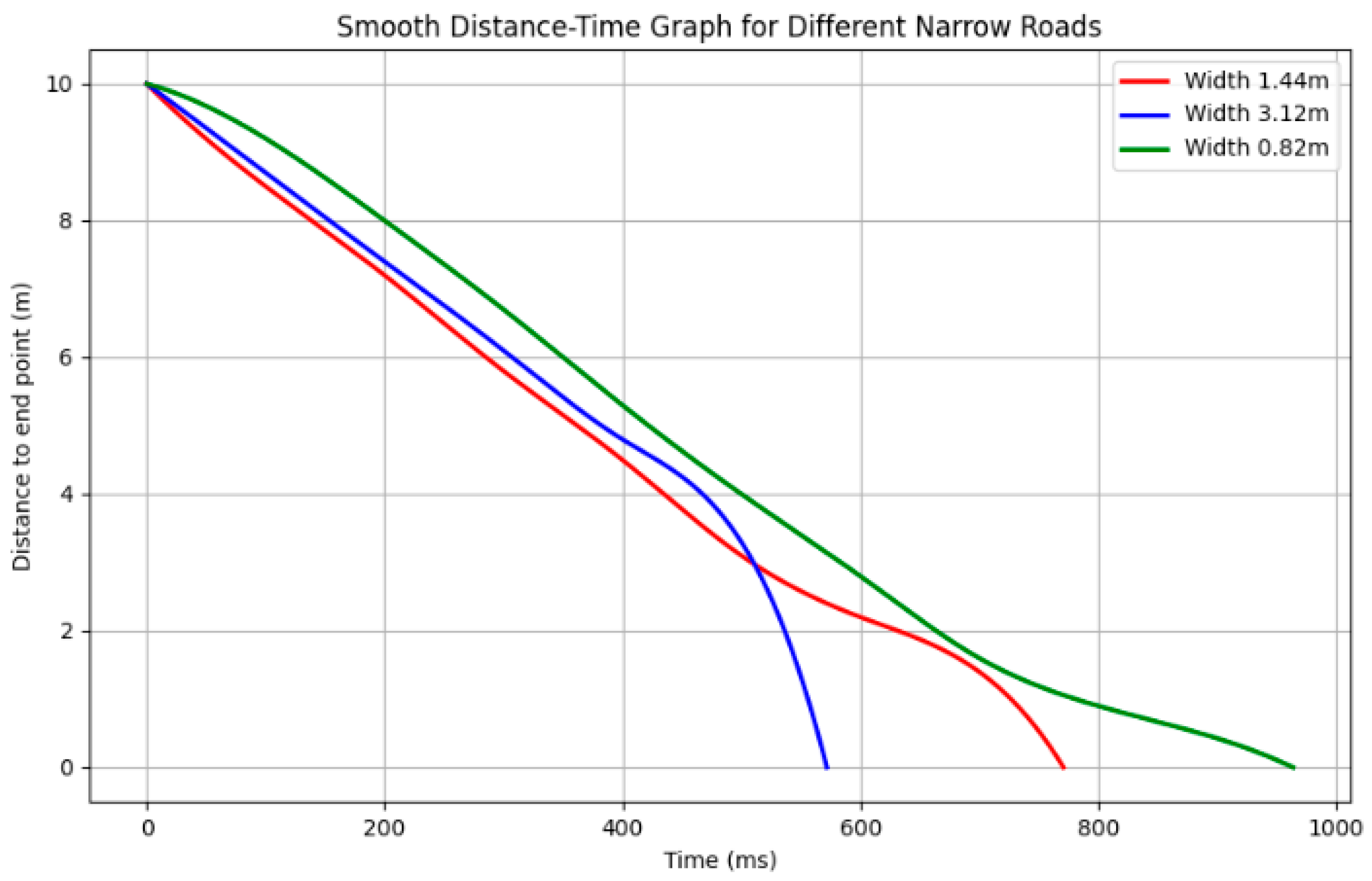
| Road Width (m) | Computation Time (ms) | Set Distance(m) | Curvature Changes |
|---|---|---|---|
| 1.44 | 771 | 10 | 0.34412 |
| 3.12 | 572 | 10 | 0.20623 |
| 0.82 | 964 | 10 | 0.42589 |
Disclaimer/Publisher’s Note: The statements, opinions and data contained in all publications are solely those of the individual author(s) and contributor(s) and not of MDPI and/or the editor(s). MDPI and/or the editor(s) disclaim responsibility for any injury to people or property resulting from any ideas, methods, instructions or products referred to in the content. |
© 2025 by the authors. Licensee MDPI, Basel, Switzerland. This article is an open access article distributed under the terms and conditions of the Creative Commons Attribution (CC BY) license (https://creativecommons.org/licenses/by/4.0/).
Share and Cite
Wang, P.; Zhang, H.; Tang, Y. Path Planning in Narrow Road Scenarios Based on Four-Layer Network Cost Structure Map. Sensors 2025, 25, 2786. https://doi.org/10.3390/s25092786
Wang P, Zhang H, Tang Y. Path Planning in Narrow Road Scenarios Based on Four-Layer Network Cost Structure Map. Sensors. 2025; 25(9):2786. https://doi.org/10.3390/s25092786
Chicago/Turabian StyleWang, Ping, Hao Zhang, and Youming Tang. 2025. "Path Planning in Narrow Road Scenarios Based on Four-Layer Network Cost Structure Map" Sensors 25, no. 9: 2786. https://doi.org/10.3390/s25092786
APA StyleWang, P., Zhang, H., & Tang, Y. (2025). Path Planning in Narrow Road Scenarios Based on Four-Layer Network Cost Structure Map. Sensors, 25(9), 2786. https://doi.org/10.3390/s25092786