Underwater Target Recognition Method Based on Singular Spectrum Analysis and Channel Attention Convolutional Neural Network


Abstract
1. Introduction
- (1)
- The paper proposes a novel approach that integrates the conventional rapid SSA signal decomposition method with the deep attention convolutional neural network. This integration contributes to enhancing the efficiency of underwater acoustic target recognition. The model exhibits a certain degree of robustness in the case of a relatively low SNR.
- (2)
- The front end of the SSA-CACNN deep neural network model uses the SSA method that can directly process raw time-domain underwater acoustic signals. The decomposition process significantly reduces the impact of noise. The back end incorporates a channel attention mechanism to weight signal features, enhancing the model’s ability to extract the essential characteristics of the signals.
- (3)
- In the SSA-CACNN deep neural network model, the front-end SSA component requires only the first three components to reconstruct the original signal. Compared to other methods, this approach helps reduce the number of network parameters and lowers the overall complexity of the network.
2. SSA Module Design and Principles
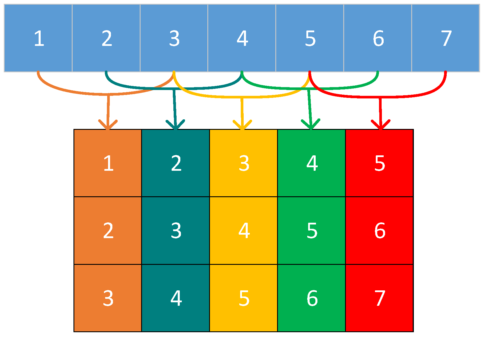
2.1. Signal Preprocessing Module
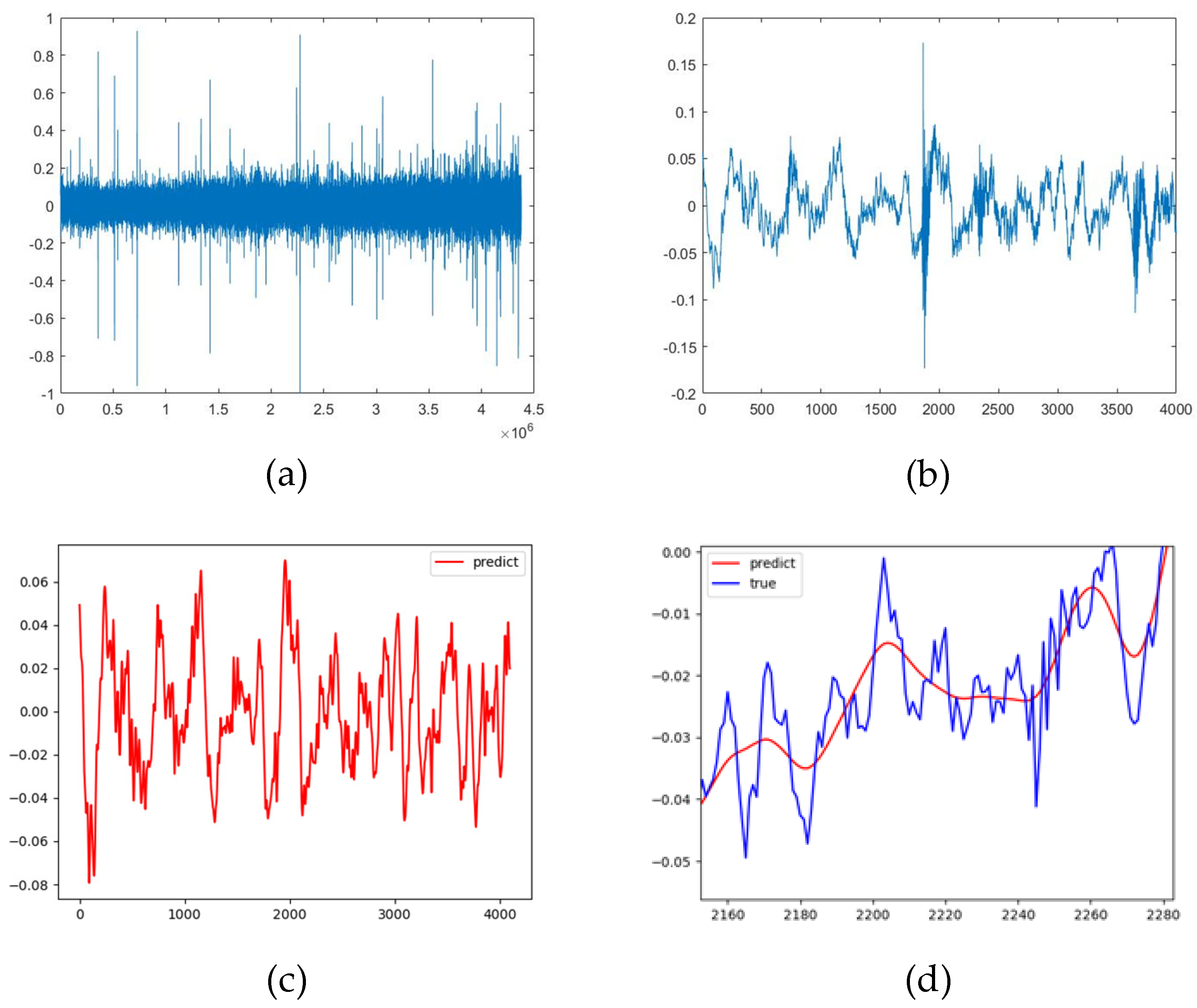
2.2. Decomposition and Reconstruction Module
3. CACNN Model Construction
3.1. Fundamental Principles of Convolutional Neural Network (CNN)
- Convolutional layer
- 2.
- Pooling Layer
- 3.
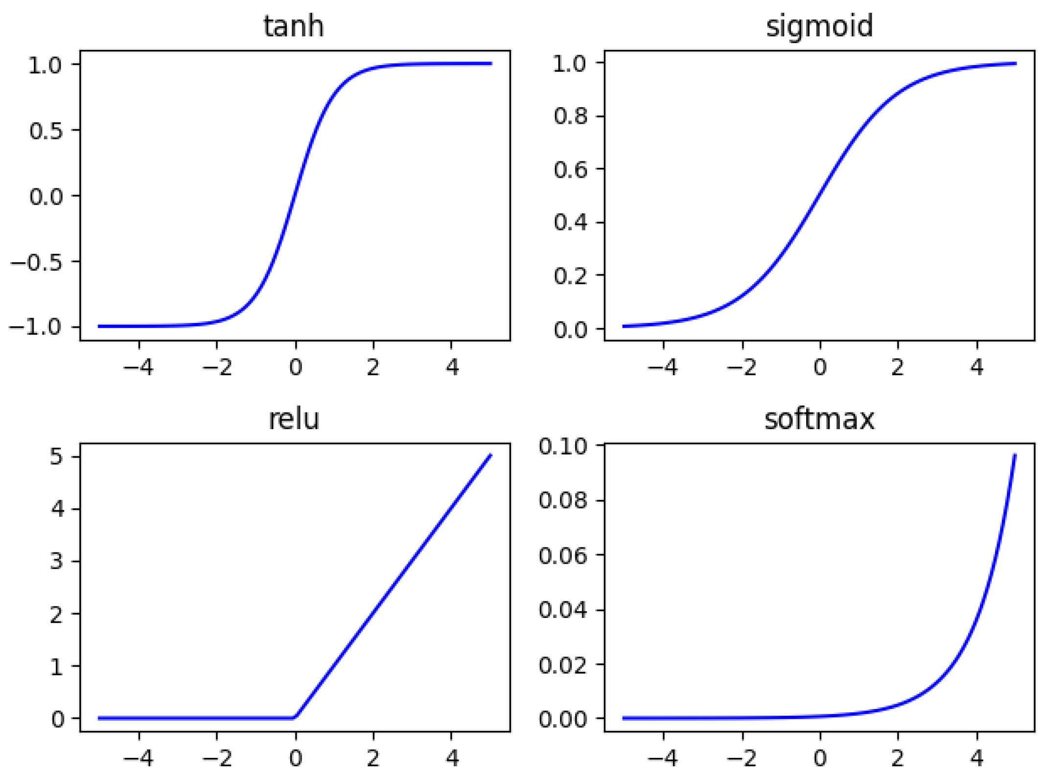
- Activation Function
- 4.
- Fully Connected Layer
- 5.
- Classification Layer
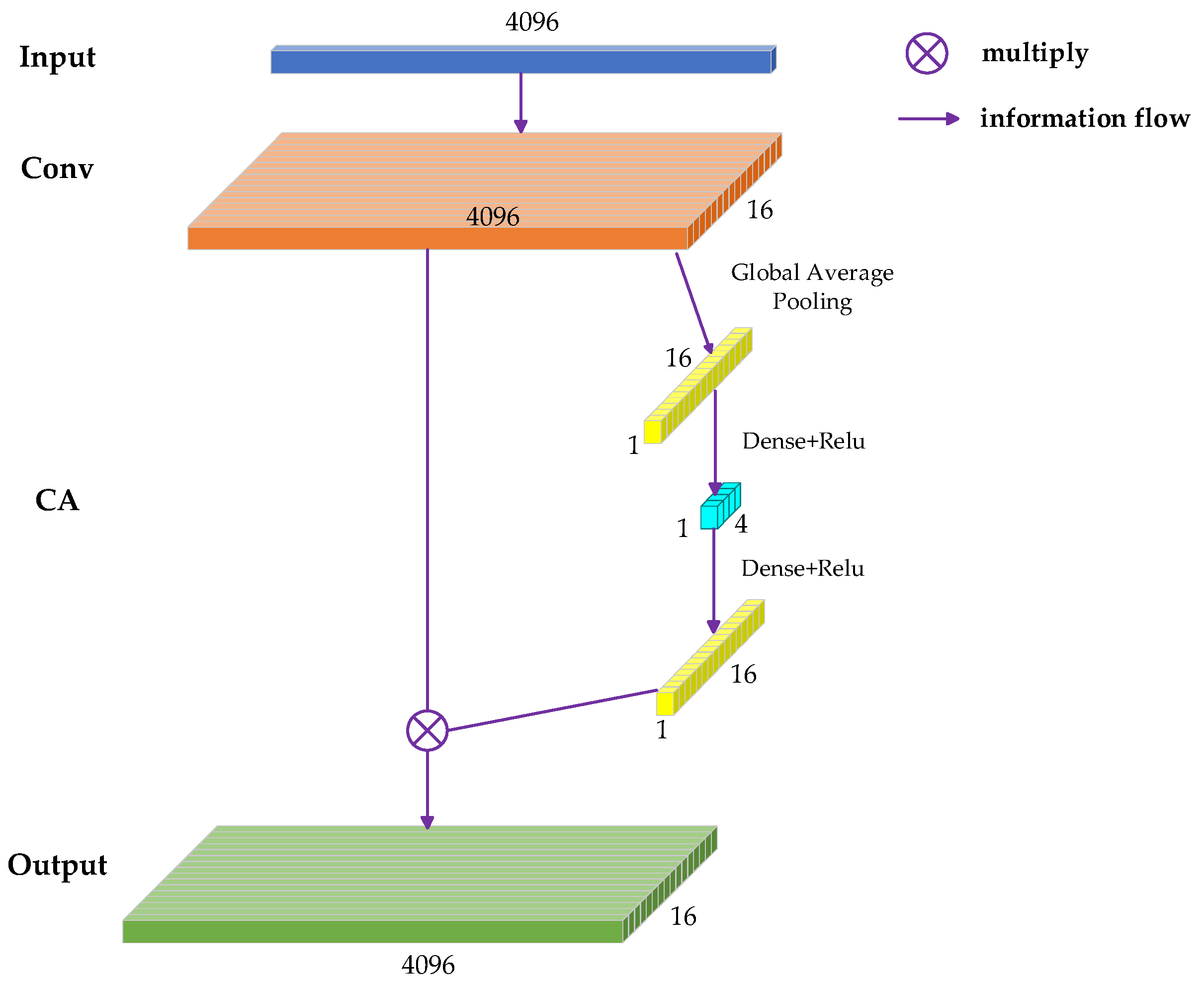
3.2. Attention Mechanism Module
3.3. SSA-CACNN-Based Underwater Acoustic Target Recognition Model
4. Experimental Results Analysis
4.1. Dataset and Sample Set
4.2. Experimental Results and Analysis
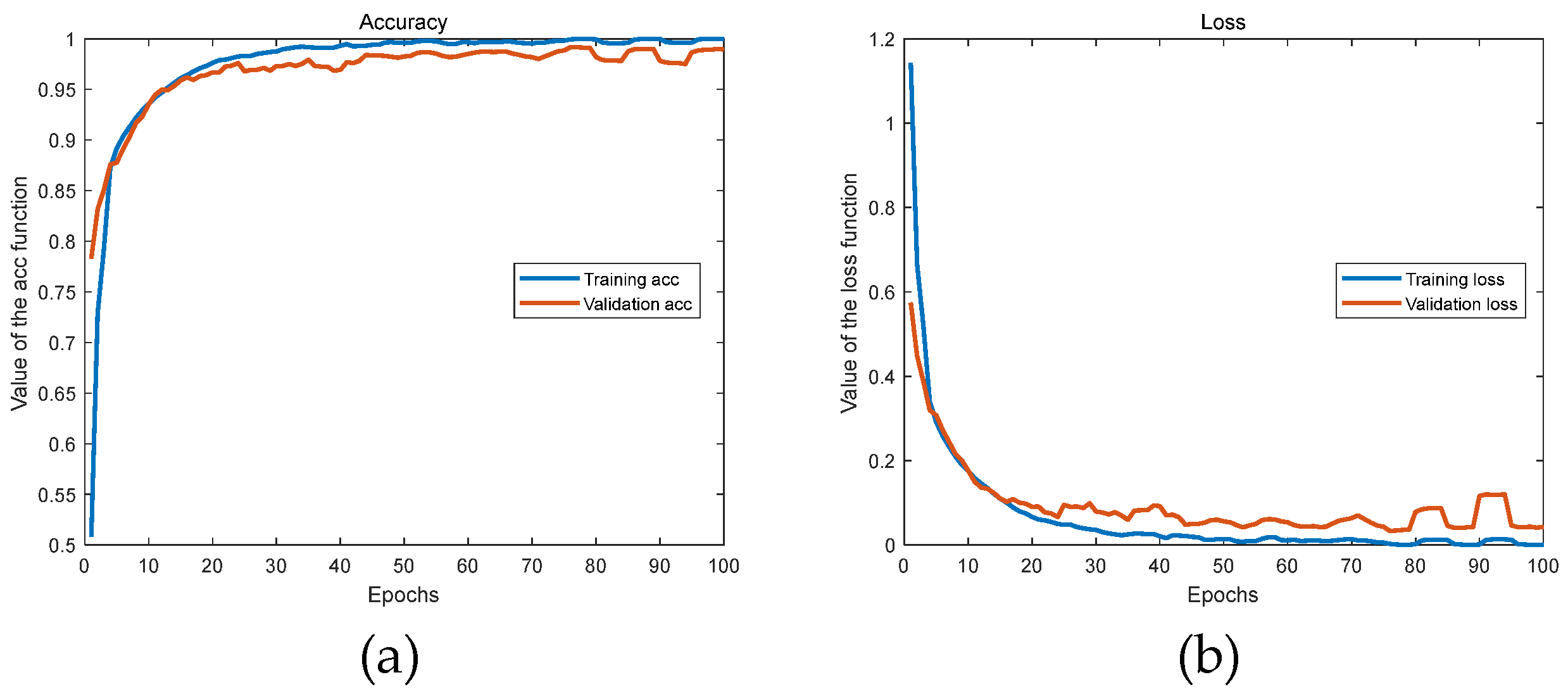
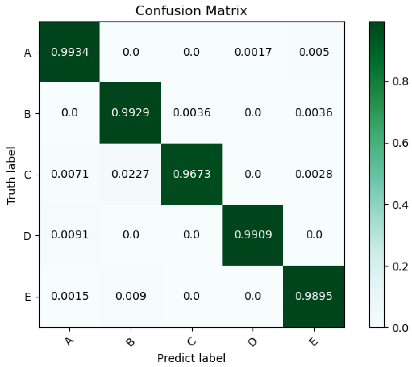
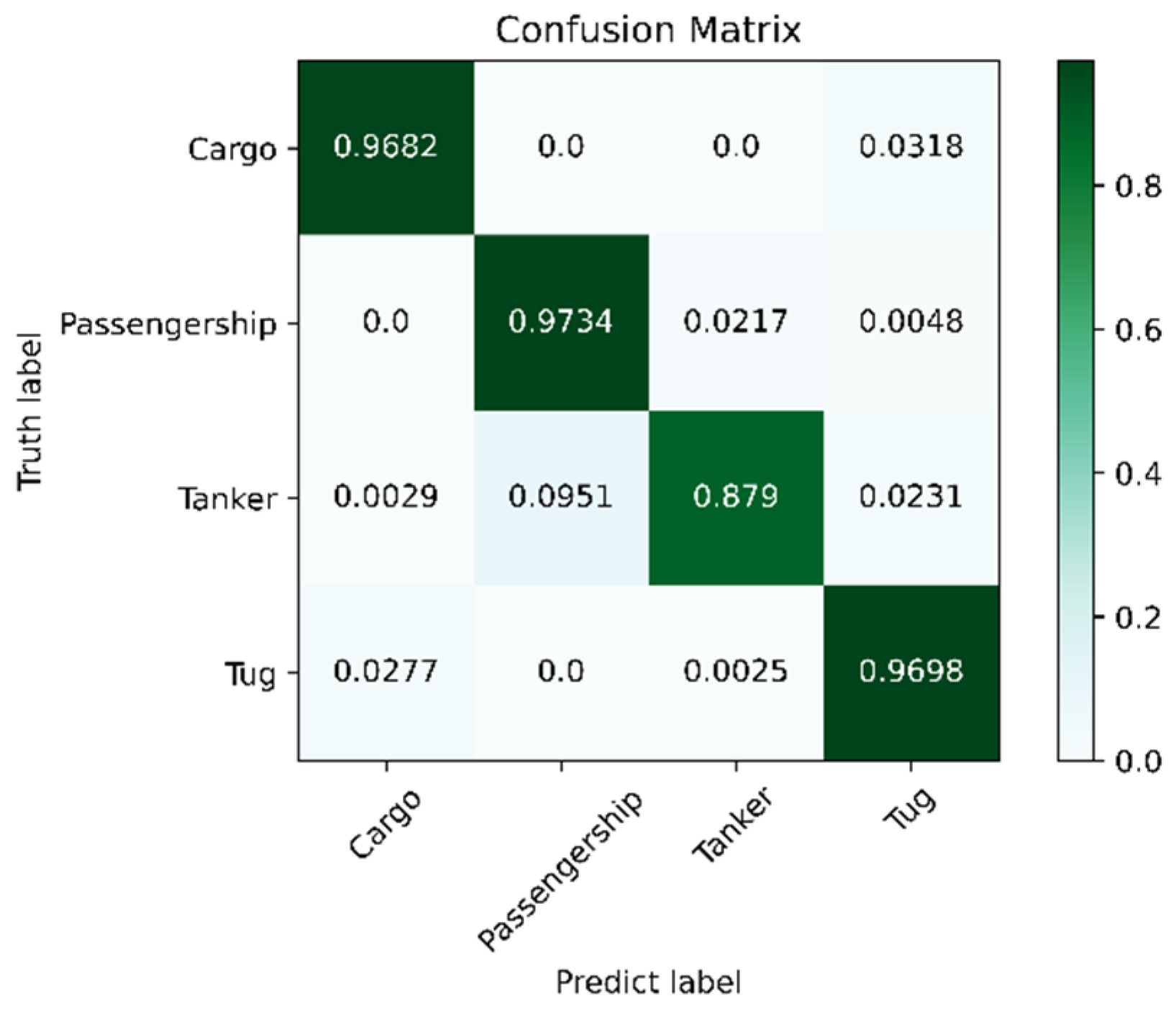
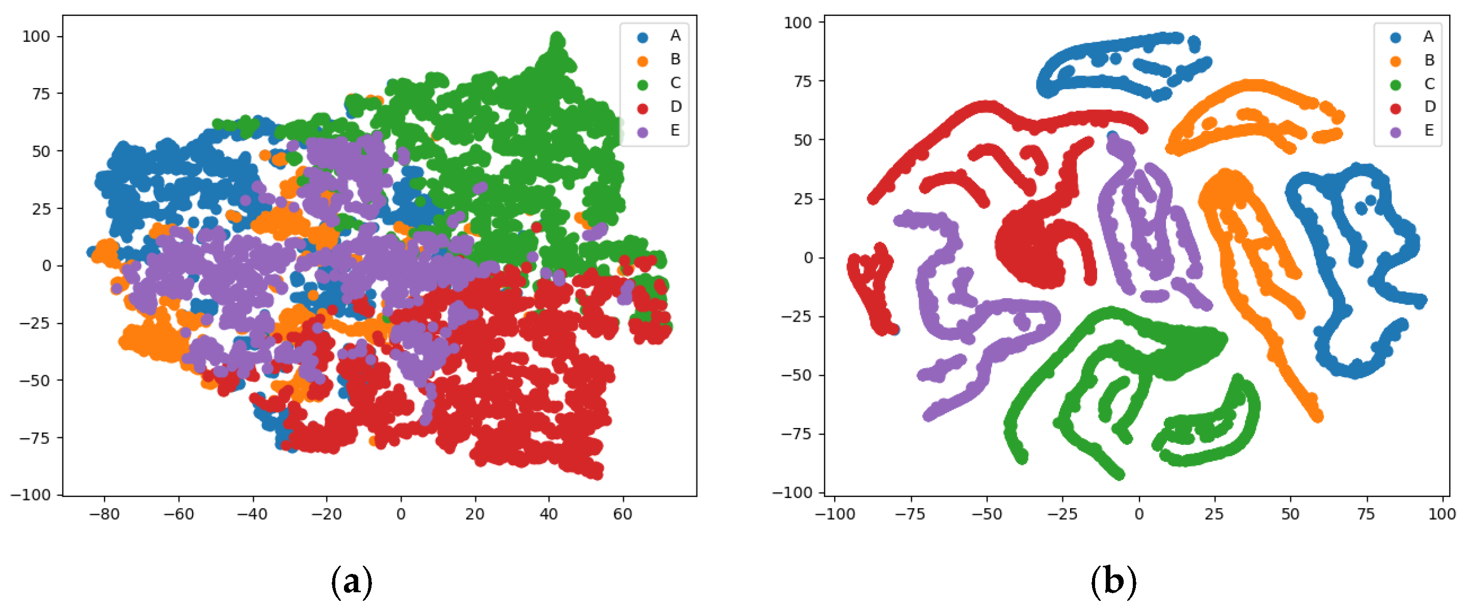
4.2.1. The Classification and Recognition Results of the Model
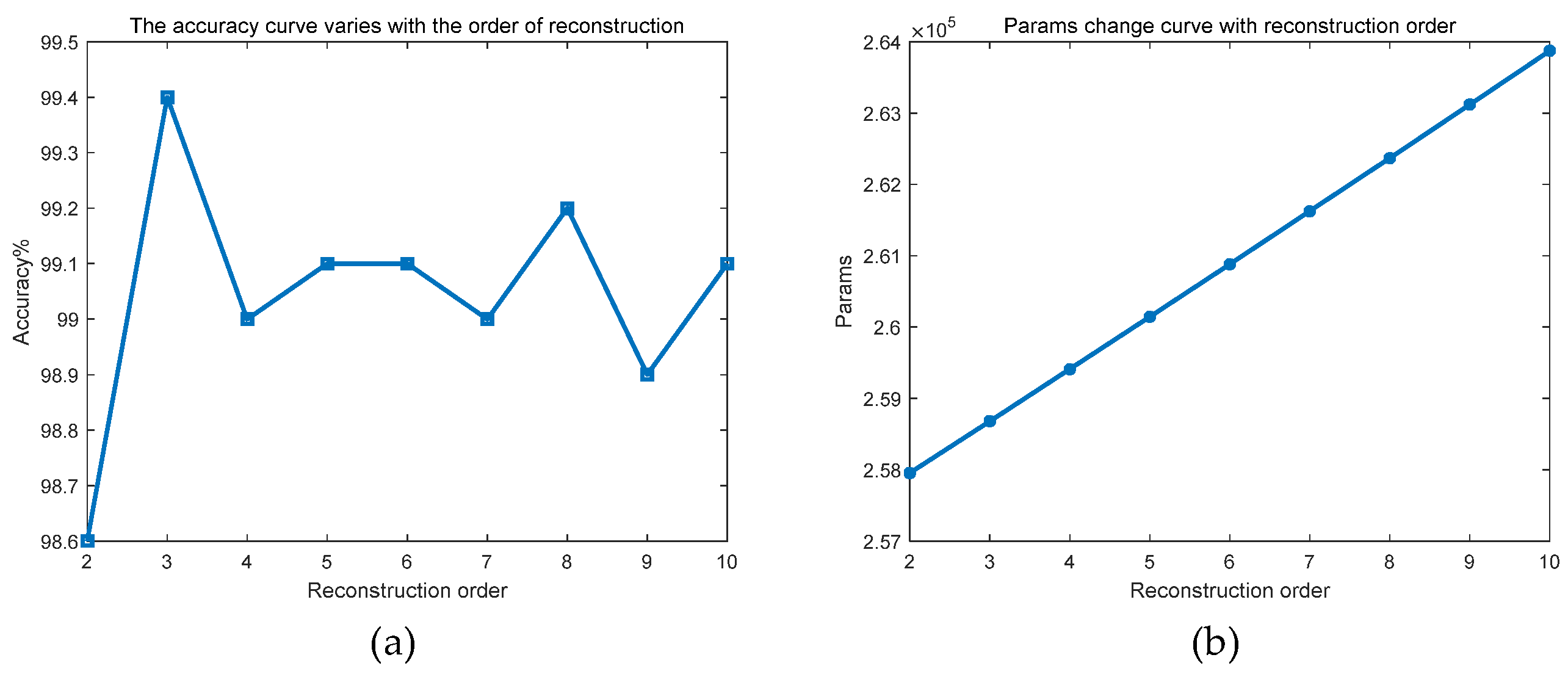
4.2.2. The Influence of the Order of Reconstructed Signals
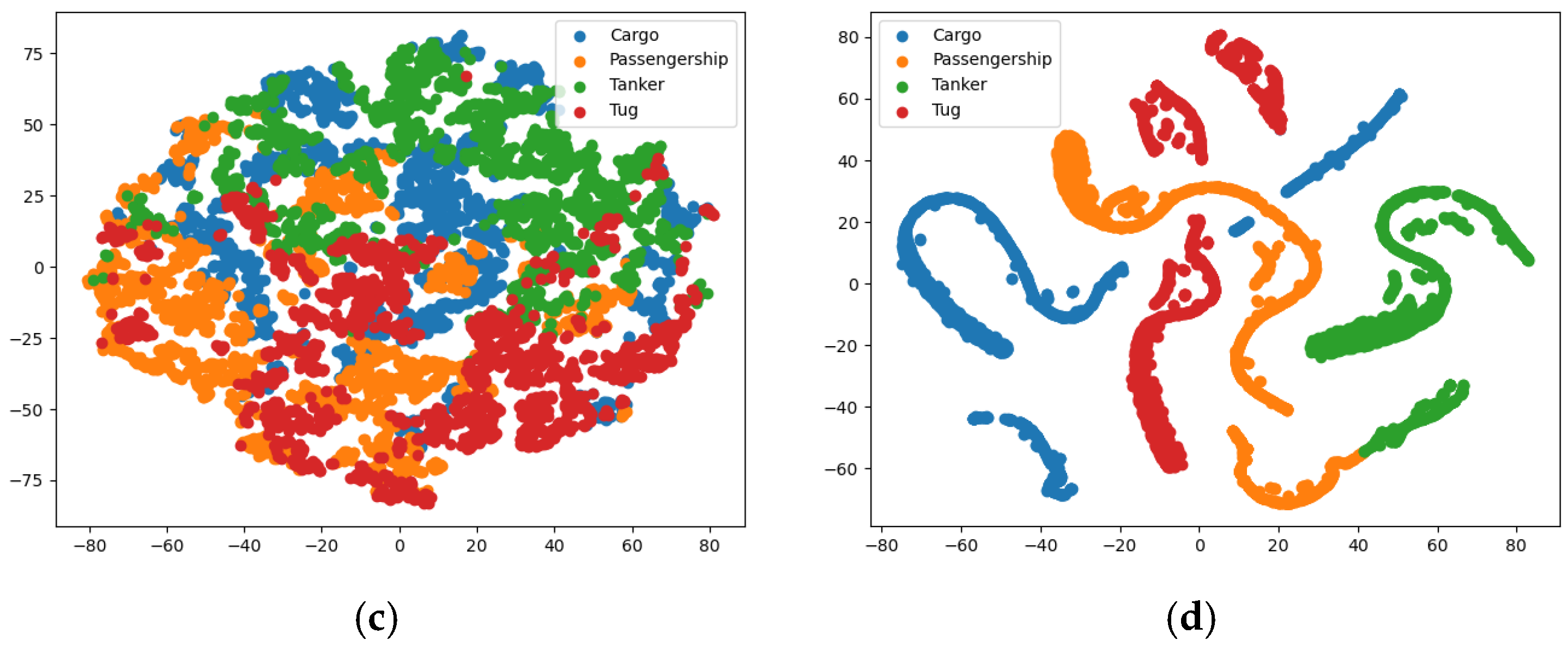
4.2.3. Robustness After Adding Noise
5. Conclusions
Author Contributions
Funding
Institutional Review Board Statement
Informed Consent Statement
Data Availability Statement
Acknowledgments
Conflicts of Interest
References
- Li, P.; Wu, J.; Wang, Y.; Lan, Q.; Xiao, W. STM: Spectrogram Transformer Model for Underwater Acoustic Target Recognition. J. Mar. Sci. Eng. 2022, 10, 1428. [Google Scholar] [CrossRef]
- Jiang, J.; Wu, Z.; Lu, J.; Huang, M.; Xiao, Z. Interpretable features for underwater acoustic target recognition. Measurement 2021, 173, 108586. [Google Scholar] [CrossRef]
- Jiang, J.; Shi, T.; Huang, M.; Xiao, Z. Multi-scale spectral feature extraction for underwater acoustic target recognition. Measurement 2020, 166, 108227. [Google Scholar] [CrossRef]
- Ji, F.; Li, G.; Lu, S.; Ni, J. Research on a Feature Enhancement Extraction Method for Underwater Targets Based on Deep Autoencoder Networks. Appl. Sci. 2024, 14, 1341. [Google Scholar] [CrossRef]
- Jin, S.Y.; Su, Y.; Guo, C.J.; Fan, Y.X.; Tao, Z.Y. Offshore ship recognition based on center frequency projection of improved EMD and KNN algorithm. Mech. Syst. Signal Process. 2023, 189, 110076. [Google Scholar] [CrossRef]
- Wang, R.R.; Xiang, M.S.; Li, C. Denoising FMCW Ladar Signals via EEMD With Singular Spectrum Constraint. IEEE Geosci. Remote Sens. Lett. 2020, 17, 983–987. [Google Scholar] [CrossRef]
- Hu, S.G.; Zhang, L.; Tang, J.T.; Li, G.; Yang, H.Y.; Xu, Z.H.; Zhang, L.C.; Xiang, J.N. Identification of the Shaft-Rate Electromagnetic Field Induced by a Moving Ship Using Improved Learning-Based and Spectral-Direction Methods. IEEE Trans. Geosci. Remote Sens. 2024, 62, 5922511. [Google Scholar] [CrossRef]
- Dai, T.; Xu, S.; Tian, B.; Hu, J.; Zhang, Y.; Chen, Z. Extraction of Micro-Doppler Feature Using LMD Algorithm Combined Supplement Feature for UAVs and Birds Classification. Remote Sens. 2022, 14, 2196. [Google Scholar] [CrossRef]
- Lin, Y.; Ling, B.W.-K.; Hu, L.; Zheng, Y.; Xu, N.; Zhou, X.; Wang, X. Hyperspectral Image Enhancement by Two Dimensional Quaternion Valued Singular Spectrum Analysis for Object Recognition. Remote Sens. 2021, 13, 405. [Google Scholar] [CrossRef]
- Zhu, S.; Gao, W.; Li, X. SSANet: Normal-mode interference spectrum extraction via SSA algorithm-unrolled neural network. Front. Mar. Sci. 2024, 10, 1342090. [Google Scholar] [CrossRef]
- Golyandina, N. Particularities and commonalities of singular spectrum analysis as a method of time series analysis and signal processing. Wiley Interdiscip. Rev.-Comput. Stat. 2020, 12, e1487. [Google Scholar] [CrossRef]
- Jain, S.; Panda, R.; Tripathy, R.K. Multivariate Sliding-Mode Singular Spectrum Analysis for the Decomposition of Multisensor Time Series. IEEE Sens. Lett. 2020, 4, 7002404. [Google Scholar] [CrossRef]
- Haghbin, H.; Najibi, S.M.; Mahmoudvand, R.; Trinka, J.; Maadooliat, M. Functional singular spectrum analysis. Stat 2021, 10, e330. [Google Scholar] [CrossRef]
- Guo, F. Underwater Acoustic Signal Denoising Algorithm Based on Improved EEMD and VMD. Master’s Thesis, North University of China, Shanxi, China, 2022. [Google Scholar]
- Gu, J.; Hung, K.; Ling, B.; Chow, D.; Zhou, Y.; Fu, Y.; Pun, S. Generalized singular spectrum analysis for the decomposition and analysis of non-stationary signals. J. Frankl. Inst. 2024, 361, 106696. [Google Scholar] [CrossRef]
- Bao, F.; Wang, X.; Tao, Z.; Wang, Q.; Du, S. Adaptive extraction of modulation for cavitation noise. J. Acoust. Soc. Am. 2009, 126, 3106–3113. [Google Scholar] [CrossRef]
- Lei, M.; Zeng, X.; Jin, A.; Yang, S.; Wang, H. Low-Frequency Noise Suppression Based on Mode Decomposition and Low-Rank Matrix Approximation for Underwater Acoustic Target Signal. IEEE Trans. Geosci. Remote Sens. 2024, 62, 4209012. [Google Scholar] [CrossRef]
- Chen, L.; Luo, X.; Zhou, H.; Shen, Q.; Chen, L.; Huan, C. Underwater acoustic multi-target recognition based on channel attention mechanism. Ocean. Eng. 2025, 315, 119841. [Google Scholar] [CrossRef]
- Chen, L.; Luo, X.; Zhou, H. A ship-radiated noise classification method based on domain knowledge embedding and attention mechanism. Eng. Appl. Artif. Intell. 2024, 127, 107320. [Google Scholar] [CrossRef]
- Yang, S.; Jin, A.; Zeng, X.; Wang, H.; Hong, X.; Lei, M. Underwater acoustic target recognition based on sub-band concatenated Mel spectrogram and multidomain attention mechanism. Eng. Appl. Artif. Intell. 2024, 133, 107983. [Google Scholar] [CrossRef]
- Chen, Z.; Xie, G.; Chen, M.; Qiu, H. Model for Underwater Acoustic Target Recognition with Attention Mechanism Based on Residual Concatenate. J. Mar. Sci. Eng. 2024, 12, 24. [Google Scholar] [CrossRef]
- Jin, A.; Zeng, X. A Novel Deep Learning Method for Underwater Target Recognition Based on Res-Dense Convolutional Neural Network with Attention Mechanism. J. Mar. Sci. Eng. 2023, 11, 69. [Google Scholar] [CrossRef]
- Yang, K.; Wang, B.; Fang, Z.; Cai, B. An End-to-End Underwater Acoustic Target Recognition Model Based on One-Dimensional Convolution and Transformer. J. Mar. Sci. Eng. 2024, 12, 1793. [Google Scholar] [CrossRef]
- Ma, Y.; Liu, M.; Zhang, Y.; Zhang, B.; Xu, K.; Zou, B.; Huang, Z. Imbalanced Underwater Acoustic Target Recognition with Trigonometric Loss and Attention Mechanism Convolutional Network. Remote Sens. 2022, 14, 4103. [Google Scholar] [CrossRef]
- Feng, S.; Zhu, X. A Transformer-Based Deep Learning Network for Underwater Acoustic Target Recognition. IEEE Geosci. Remote Sens. Lett. 2022, 19, 1505805. [Google Scholar] [CrossRef]
- Ji, F.; Ni, J.S.; Li, G.N.; Liu, L.L.; Wang, Y.Y. Underwater Acoustic Target Recognition Based on Deep Residual Attention Convolutional Neural Network. J. Mar. Sci. Eng. 2023, 11, 1626. [Google Scholar] [CrossRef]
- Luo, Y.; Kuang, C.; Lu, C.; Zeng, F. GPS Coordinate Series Denoising and Seasonal Signal Extraction Based on SSA. J. Geod. Geodyn. 2015, 35, 391–395. [Google Scholar] [CrossRef]
- Ni, J.; Ji, F.; Lu, S.; Feng, W. An Auditory Convolutional Neural Network for Underwater Acoustic Target Timbre Feature Extraction and Recognition. Remote Sens. 2024, 16, 3074. [Google Scholar] [CrossRef]
- Woo, S.; Park, J.; Lee, J.Y.; Kweon, I.S. CBAM: Convolutional Block Attention Module. In Computer Vision—ECCV 2018; Lecture Notes in Computer Science; Springer: Cham, Switzerland, 2018; Volume 11211, pp. 3–19. [Google Scholar] [CrossRef]
- David, S.D.; Soledad, T.G.; Antonio, C.L.; Antonio, P.G. ShipsEar: An underwater vessel noise database. Appl. Acoust. 2016, 113, 64–69. [Google Scholar] [CrossRef]
- Hong, F.; Liu, C.W.; Guo, L.J.; Chen, F.; Feng, H.H. Underwater Acoustic Target Recognition with a Residual Network and the Optimized Feature Extraction Method. Appl. Sci. 2021, 11, 1442. [Google Scholar] [CrossRef]
- Li, J.; Wang, B.X.; Cui, X.R.; Li, S.B.; Liu, J.H. Underwater Acoustic Target Recognition Based on Attention Residual Network. Entropy 2022, 24, 1657. [Google Scholar] [CrossRef]
- Irfan, M.; Zheng, J.B.; Ali, S.; Iqbal, M.; Masood, Z. DeepShip: An underwater acoustic benchmark dataset and a separable convolution based autoencoder for classification. Expert Syst. Appl. 2021, 183, 115270. [Google Scholar] [CrossRef]


| SSA Operating Procedures | |
|---|---|
| Step1 | Embedding—forming a trajectory matrix. |
| Step2 | Decomposition—SVD for signal decomposition. |
| Step3 | Grouping—grouping the features. |
| Step4 | Refactoring—obtain denoised signal after reconstruction (if all components are summed, the reconstructed signal will be the original signal, albeit with minor errors). |
| Layer | Input Shape | Output Shape |
|---|---|---|
| Input | (None, 4096, 3) | (None, 4096, 3) |
| CA | (None, 4096, 3) | (None, 4096, 3) (None, 1, 3) |
| Conv1D | (None, 4096, 1) | (None, 4096, 16) |
| CA | (None, 4096, 16) | (None, 4096, 16) (None, 1, 16) |
| Conv1D | (None, 1024, 16) | (None, 1024, 32) |
| GAP | (None, 1024, 32) | (None, 32) |
| Conv1D | (None, 256, 32) | (None, 64, 128) |
| Conv1D | (None, 64, 128) | (None, 32, 128) |
| Conv1D | (None, 32, 128) | (None, 16, 128) |
| GAP | (None, 16, 128) | (None, 128) |
| Dense | (None, 128) | (None, 5) |
| Output | (None, 5) | (None, 5) |
| Category | Type of Vessel | Files | Duration (s) |
|---|---|---|---|
| Class A | Fishing boats, trawlers, mussel boats, tugboats, dredgers | 17 | 1880 |
| Class B | Motorboats, pilot boats, sailboats | 19 | 1567 |
| Class C | Passenger ferries | 30 | 4276 |
| Class D | Ocean liners, RORO vessels | 12 | 2460 |
| Class E | Background noise recordings | 12 | 1145 |
| Categories | Accuracy (%) | Precision (%) | Recall (%) | F1-Score (%) |
|---|---|---|---|---|
| A | 99.34 | 97.88 | 99.34 | 98.6 |
| B | 99.29 | 96.21 | 99.29 | 97.72 |
| C | 96.73 | 99.71 | 96.73 | 98.2 |
| D | 99.09 | 99.87 | 99.09 | 99.48 |
| E | 98.95 | 98.95 | 98.95 | 98.95 |
| Average | 98.68 | 98.52 | 98.68 | 98.59 |
| No. | Method | Accuracy (%) | Params (M) |
|---|---|---|---|
| 1 | ResNet-18 [31] | 94.9 | 0.78 |
| 2 | AResNet [32] | 98.0 | 9.47 |
| 3 | DRACNN [26] | 97.1 | 0.26 |
| 4 | SE_ResNet [18] | 98.09 | \ |
| 5 | HUAT [19] | 98.62 | 30.3 |
| 6 | CFTANet [20] | 96.4 | 0.47 |
| 7 | ARescat [21] | 95.8 | \ |
| 8 | 1DCTN [23] | 96.84 | 0.45 |
| 9 | MR-CNN-A [24] | 98.87 | \ |
| 10 | UATR-transformer [25] | 96.9 | 2.55 |
| 11 | ACNN_DRACNN [28] | 99.87 | 0.61 |
| 12 | SSA-CACNN (the proposed method) | 98.64 | 0.26 |
| Categories | Accuracy (%) | Precision (%) | Recall (%) | F1-Score (%) |
|---|---|---|---|---|
| Cargo | 96.82 | 96.82 | 96.82 | 96.82 |
| Passenger Ship | 97.34 | 92.43 | 97.34 | 94.82 |
| Tanker | 87.9 | 96.83 | 87.9 | 92.15 |
| Tug | 96.98 | 94.59 | 96.98 | 95.77 |
| Average | 94.76 | 95.17 | 94.76 | 94.89 |
| Reconstruction Order | Accuracy | Params |
|---|---|---|
| 2 | 98.6% | 257,954 |
| 3 | 99.4% | 258,680 |
| 4 | 99.0% | 259,410 |
| 5 | 99.1% | 260,144 |
| 6 | 99.1% | 260,882 |
| 7 | 99.0% | 261,624 |
| 8 | 99.2% | 262,370 |
| 9 | 98.9% | 263,120 |
| 10 | 99.1% | 263,874 |
Disclaimer/Publisher’s Note: The statements, opinions and data contained in all publications are solely those of the individual author(s) and contributor(s) and not of MDPI and/or the editor(s). MDPI and/or the editor(s) disclaim responsibility for any injury to people or property resulting from any ideas, methods, instructions or products referred to in the content. |
© 2025 by the authors. Licensee MDPI, Basel, Switzerland. This article is an open access article distributed under the terms and conditions of the Creative Commons Attribution (CC BY) license (https://creativecommons.org/licenses/by/4.0/).
Share and Cite
Ji, F.; Lu, S.; Ni, J.; Li, Z.; Feng, W. Underwater Target Recognition Method Based on Singular Spectrum Analysis and Channel Attention Convolutional Neural Network. Sensors 2025, 25, 2573. https://doi.org/10.3390/s25082573
Ji F, Lu S, Ni J, Li Z, Feng W. Underwater Target Recognition Method Based on Singular Spectrum Analysis and Channel Attention Convolutional Neural Network. Sensors. 2025; 25(8):2573. https://doi.org/10.3390/s25082573
Chicago/Turabian StyleJi, Fang, Shaoqing Lu, Junshuai Ni, Ziming Li, and Weijia Feng. 2025. "Underwater Target Recognition Method Based on Singular Spectrum Analysis and Channel Attention Convolutional Neural Network" Sensors 25, no. 8: 2573. https://doi.org/10.3390/s25082573
APA StyleJi, F., Lu, S., Ni, J., Li, Z., & Feng, W. (2025). Underwater Target Recognition Method Based on Singular Spectrum Analysis and Channel Attention Convolutional Neural Network. Sensors, 25(8), 2573. https://doi.org/10.3390/s25082573