
Circle Detection with Adaptive Parameterization: A Bottom-Up Approach


Abstract
1. Introduction
2. Methodology
2.1. Edge Point Detection
2.2. The pRC Algorithm
2.2.1. Edge Points Partitioning
2.2.2. RANSAC on Patches
| Algorithm 1: The pRC algorithm | |
| : All edge points in patch | |
| 1 | Calculate the loop count N using (1–2) |
| 2 | |
| 3 | |
| 4 | //for line segments, t = 2; for circular arcs, t = 3 |
| 5 | , THEN CONTINUE |
| 6 | |
| 7 | |
| 8 | |
| 9 | |
| 10 | THEN GOTO line 15 |
| 11 | |
| 12 | |
| 13 | |
| 14 | THEN GOTO line 1 |
| 15 | |
2.2.3. Non-Maximum Suppression (NMS)
2.3. Distance Metric
2.4. The HS Algorithm
| Algorithm 2: Calculate candidate circle parameters | |
| : : All segments derived from section C. | |
| : | |
| 1 | //: A function that fits circular parameters via least squares, returns parameters if its distance criterion is met, see Equations (6) and (7); otherwise, returns None. |
| 2 | |
| 3 | |
| 4 | |
| 5 | |
| 6 | |
| 7 | Q |
| 8 | |
| 9 | |
| 10 | < |
| 11 | End FOR EACH |
| 12 | THEN: |
| 13 | |
| 14 | |
| 15 | |
| 16 | THEN: |
| 17 | End FOR EACH |
| 18 | THEN: |
| 19 | |
| 20 | GOTO line 2 |
| 21 | End IF |
| 22 | |
2.5. The CPS Algorithm
| Algorithm 3: Circle Space Refinement | |
| : : Circle parameter library | |
| : Refined Circles | |
| 1 | |
| 2 | FOR EACH in : |
| 3 | |
| 4 | |
| 5 | //Select the circle minimizing the distance metric defined in Equation (6). |
| 6 | IF THEN CONTINUE |
| 7 | |
| 8 | |
| 9 | END FOR EACH |
| 10 | |
| 11 | IF THEN |
| 12 | |
| 13 | GOTO line 1 |
| 14 | END IF |
| 15 | RETURN |
2.6. Arc Length Ratio Criteria
3. Experiments and Results
3.1. Datasets
- Dataset-Mini: A benchmark test set containing 10 low-resolution images with fixed pixel dimensions, presenting spectral reflection and occlusion challenges, originally established by Akinlar and Topal [11].
- Dataset-GH: A complex real-world collection of 258 grayscale images from diverse environments, exhibiting blurred boundaries, partial occlusions, and substantial radius variations.
- Dataset-PCB: An industrial dataset comprising 100 printed circuit board (PCB) images with concentric circular structures, containing significant noise pollution and edge blurring that present detection challenges.
- Dataset-MY: A newly compiled dataset of 111 smartphone-captured images featuring multiple circular targets per frame, characterized by cluttered backgrounds, perspective distortions, and elliptical deformations caused by angular perspectives.
3.2. Environment
3.3. Comparison Metrics
3.4. Performance
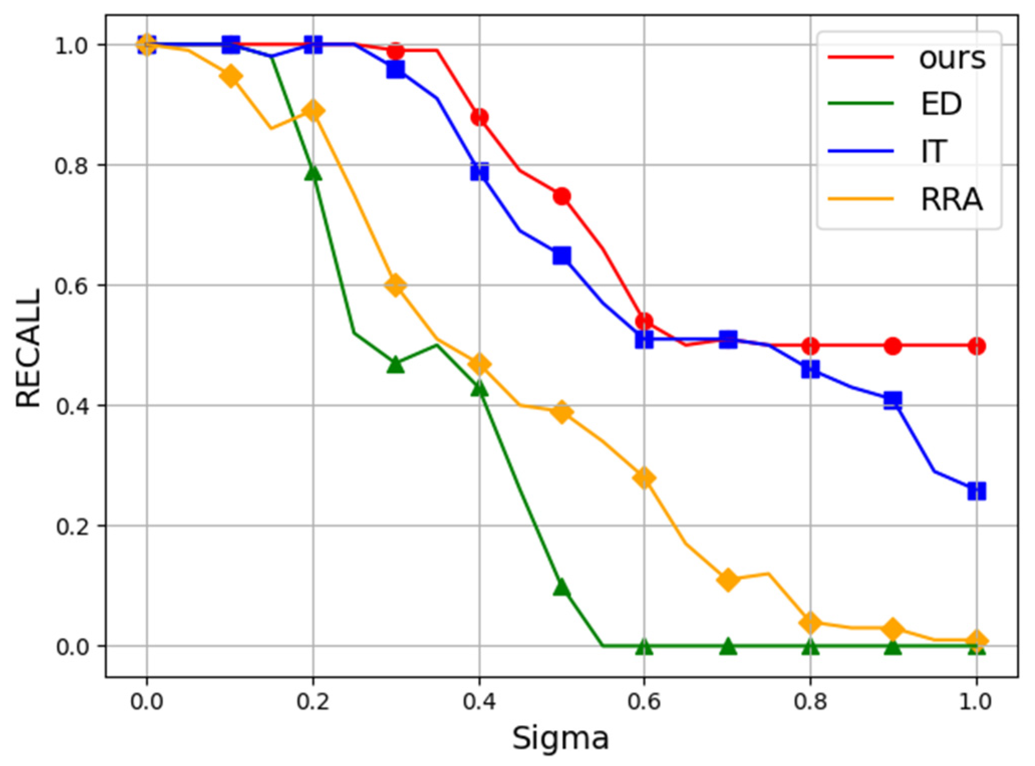
3.5. Noise Test
4. Conclusions
Author Contributions
Funding
Institutional Review Board Statement
Informed Consent Statement
Data Availability Statement
Acknowledgments
Conflicts of Interest
Abbreviations
| EDPF | Edge detection parameter-free algorithm |
| CHT | Circle Hough Transform |
| RANSAC | Random sample consensus |
| pRC | Patch-based random sample consensus algorithm |
| HS | Hierarchical search algorithm |
| CPS | Circle parameter synthesis algorithm |
Appendix A. Parameters and Their Determination Methodologies

| Parameter | Value | Explanation |
|---|---|---|
| 3 | Minimum perceptible distance discernible by human sensory capabilities. | |
| 0.05 | Minimum length difference discrimination ratio between line segments. | |
| 0.3 | An empirical parameter, employed to ascertain the minimal arc completion of an authentic circle. | |
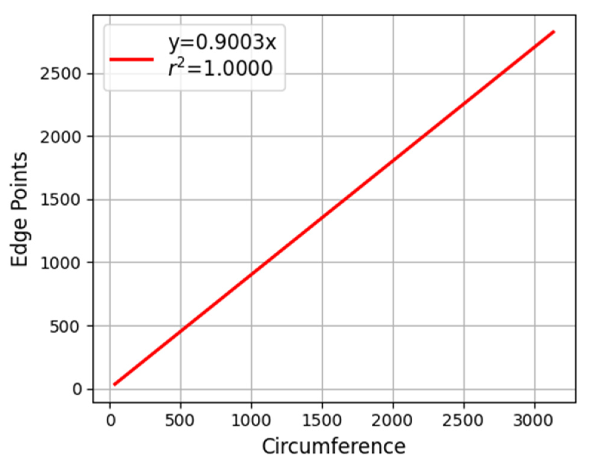
| 0.9 | Ratio between ideal and digitized circle circumferences. | |
| 16 | Minimum length of a valid line segment. | |
| 32 | Length of the side of the square area employed to identify local segments. | |
| 16 | Sliding step length of the square region utilized for detecting local segments. |
- 1.
- Value of
- 2.
- Value of
- 3.
- Value of
- 4.
- Value of
- 5.
- Value of , and
References
- Berkaya, S.K.; Gunduz, H.; Ozsen, O.; Akinlar, C.; Gunal, S. On Circular Traffic Sign Detection and Recognition. Expert Syst. Appl. 2016, 48, 67–75. [Google Scholar] [CrossRef]
- Jovančević, I.; Larnier, S.; Orteu, J.-J.; Sentenac, T. Automated Exterior Inspection of an Aircraft with a Pan-Tilt-Zoom Camera Mounted on a Mobile Robot. J. Electron. Imaging 2015, 24, 061110. [Google Scholar] [CrossRef]
- Xu, R.; Zhao, X.; Liu, F.; Tao, B. High-Precision Monocular Vision Guided Robotic Assembly Based on Local Pose Invariance. IEEE Trans. Instrum. Meas. 2023, 72, 1–12. [Google Scholar] [CrossRef]
- Alomari, Y.M.; Sheikh Abdullah, S.N.H.; Zaharatul Azma, R.; Omar, K. Automatic Detection and Quantification of WBCs and RBCs Using Iterative Structured Circle Detection Algorithm. Comput. Math. Methods Med. 2014, 2014, 979302. [Google Scholar] [CrossRef]
- Puente, J.M.R.; Garnica, J.M.R.; Isáis, C.A.G. Measuring Hardness System Based on Image Processing. In Proceedings of the 2024 21st International Conference on Electrical Engineering, Computing Science and Automatic Control (CCE), Mexico City, Mexico, 23–25 October 2024; IEEE: Piscataway, NJ, USA, 2024; pp. 1–5. [Google Scholar]
- Ou, Y.; Deng, H.; Liu, Y.; Zhang, Z.; Lan, X. An Anti-Noise Fast Circle Detection Method Using Five-Quadrant Segmentation. Sensors 2023, 23, 2732. [Google Scholar] [CrossRef]
- Xu, X.; Yang, R.; Wang, N. A Robust Circle Detector with Regionalized Radius Aid. Pattern Recognit. 2024, 149, 110256. [Google Scholar] [CrossRef]
- Guo, J.; Yang, Y.; Xiong, X.; Yang, Y.; Shao, M. Brake Disc Positioning and Defect Detection Method Based on Improved Canny Operator. IET Image Process. 2024, 18, 1283–1295. [Google Scholar] [CrossRef]
- Yang, K.; Yu, L.; Xia, M.; Xu, T.; Li, W. Nonlinear RANSAC with Crossline Correction: An Algorithm for Vision-Based Curved Cable Detection System. Opt. Lasers Eng. 2021, 141, 106417. [Google Scholar] [CrossRef]
- Meng, Y.; Zhang, Z.; Yin, H.; Ma, T. Automatic Detection of Particle Size Distribution by Image Analysis Based on Local Adaptive Canny Edge Detection and Modified Circular Hough Transform. Micron 2018, 106, 34–41. [Google Scholar] [CrossRef]
- Akinlar, C.; Topal, C. EDPF: A real-time parameter-free edge segment detector with a false detection control. Int. J. Patt. Recogn. Artif. Intell. 2012, 26, 1255002. [Google Scholar] [CrossRef]
- Akinlar, C.; Topal, C. EDCircles: A Real-Time Circle Detector with a False Detection Control. Pattern Recognit. 2013, 46, 725–740. [Google Scholar] [CrossRef]
- Liu, W.; Yang, X.; Sun, H.; Yang, X.; Yu, X.; Gao, H. A Novel Subpixel Circle Detection Method Based on the Blurred Edge Model. IEEE Trans. Instrum. Meas. 2021, 71, 1–11. [Google Scholar] [CrossRef]
- Zhao, M.; Jia, X.; Yan, D.-M. An Occlusion-Resistant Circle Detector Using Inscribed Triangles. Pattern Recognit. 2021, 109, 107588. [Google Scholar] [CrossRef]
- Desolneux, A.; Moisan, L.; Morel, J.-M. From Gestalt Theory to Image Analysis: A Probabilistic Approach; Springer Science & Business Media: Berlin/Heidelberg, Germany, 2007; Volume 34. [Google Scholar]
- Yao, Z.; Yi, W. Curvature Aided Hough Transform for Circle Detection. Expert Syst. Appl. 2016, 51, 26–33. [Google Scholar] [CrossRef]
- Adem, K. Exudate Detection for Diabetic Retinopathy with Circular Hough Transformation and Convolutional Neural Networks. Expert Syst. Appl. 2018, 114, 289–295. [Google Scholar] [CrossRef]
- An, Y.; Cao, Y.; Sun, Y.; Su, S.; Wang, F. Modified Hough Transform Based Registration Method for Heavy-Haul Railway Rail Profile with Intensive Environmental Noise. IEEE Trans. Instrum. Meas. 2025. early access. [Google Scholar] [CrossRef]
- Seifozzakerini, S.; Yau, W.-Y.; Mao, K.; Nejati, H. Hough Transform Implementation for Event-Based Systems: Concepts and Challenges. Front. Comput. Neurosci. 2018, 12, 103. [Google Scholar] [CrossRef]
- Smereka, M.; Dulęba, I. Circular Object Detection Using a Modified Hough Transform. Int. J. Appl. Math. Comput. Sci. 2008, 18, 85–91. [Google Scholar] [CrossRef]
- Memiş, A.; Albayrak, S.; Bilgili, F. A New Scheme for Automatic 2D Detection of Spheric and Aspheric Femoral Heads: A Case Study on Coronal MR Images of Bilateral Hip Joints of Patients with Legg-Calve-Perthes Disease. Comput. Methods Programs Biomed. 2019, 175, 83–93. [Google Scholar] [CrossRef]
- Kim, H.-S.; Kim, J.-H. A Two-Step Circle Detection Algorithm from the Intersecting Chords. Pattern Recognit. Lett. 2001, 22, 787–798. [Google Scholar] [CrossRef]
- Scitovski, R.; Majstorović, S.; Sabo, K. A Combination of RANSAC and DBSCAN Methods for Solving the Multiple Geometrical Object Detection Problem. J. Glob. Optim. 2021, 79, 669–686. [Google Scholar] [CrossRef]
- Ma, S.; Guo, P.; You, H.; He, P.; Li, G.; Li, H. An Image Matching Optimization Algorithm Based on Pixel Shift Clustering RANSAC. Inf. Sci. 2021, 562, 452–474. [Google Scholar] [CrossRef]
- Barath, D.; Matas, J. Graph-Cut RANSAC: Local Optimization on Spatially Coherent Structures. IEEE Trans. Pattern Anal. Mach. Intell. 2021, 44, 4961–4974. [Google Scholar] [CrossRef]
- Li, Z.; Shan, J. RANSAC-Based Multi Primitive Building Reconstruction from 3D Point Clouds. ISPRS J. Photogramm. Remote Sens. 2022, 185, 247–260. [Google Scholar] [CrossRef]
- Khan, R.U.; Almakdi, S.; Alshehri, M.; Haq, A.U.; Ullah, A.; Kumar, R. An Intelligent Neural Network Model to Detect Red Blood Cells for Various Blood Structure Classification in Microscopic Medical Images. Heliyon 2024, 10, e26149. [Google Scholar] [CrossRef]
- Jiang, L. A Fast and Accurate Circle Detection Algorithm Based on Random Sampling. Future Gener. Comput. Syst. 2021, 123, 245–256. [Google Scholar] [CrossRef]
- Chiu, S.-H.; Lin, K.-H.; Wen, C.-Y.; Lee, J.-H.; Chen, H.-M. A Fast Randomized Method for Efficient Circle/Arc Detection. Int. J. Innov. Comput. Inf. Control 2012, 8, 151–166. [Google Scholar]
- Lopez-Martinez, A.; Cuevas, F.J. Automatic Circle Detection on Images Using the Teaching Learning Based Optimization Algorithm and Gradient Analysis. Appl. Intell. 2019, 49, 2001–2016. [Google Scholar] [CrossRef]
- Ayala-Ramirez, V.; Garcia-Capulin, C.H.; Perez-Garcia, A.; Sanchez-Yanez, R.E. Circle Detection on Images Using Genetic Algorithms. Pattern Recognit. Lett. 2006, 27, 652–657. [Google Scholar] [CrossRef]
- Mekhalfi, M.L.; Nicolo, C.; Bazi, Y.; Rahhal, M.M.A.; Alsharif, N.A.; Maghayreh, E.A. Contrasting YOLOv5, Transformer, and EfficientDet Detectors for Crop Circle Detection in Desert. IEEE Geosci. Remote Sens. Lett. 2022, 19, 1–5. [Google Scholar] [CrossRef]
- Yue, X.; Li, H.; Shimizu, M.; Kawamura, S.; Meng, L. YOLO-GD: A Deep Learning-Based Object Detection Algorithm for Empty-Dish Recycling Robots. Machines 2022, 10, 294. [Google Scholar] [CrossRef]
- Gai, R.; Chen, N.; Yuan, H. A Detection Algorithm for Cherry Fruits Based on the Improved YOLO-v4 Model. Neural Comput. Appl. 2023, 35, 13895–13906. [Google Scholar] [CrossRef]
- Liu, G.; Nouaze, J.C.; Touko Mbouembe, P.L.; Kim, J.H. YOLO-Tomato: A Robust Algorithm for Tomato Detection Based on YOLOv3. Sensors 2020, 20, 2145. [Google Scholar] [CrossRef] [PubMed]
- Zhang, T.Y.; Suen, C.Y. A Fast Parallel Algorithm for Thinning Digital Patterns. Commun. ACM 1984, 27, 236–239. [Google Scholar] [CrossRef]
- Bentley, J.L. Multidimensional Binary Search Trees Used for Associative Searching. Commun. ACM 1975, 18, 509–517. [Google Scholar] [CrossRef]
- Yuan, H.; Hao, Y.-G.; Liu, J.-M. Research on Multi-Sensor Image Matching Algorithm Based on Improved Line Segments Feature. In Proceedings of the ITM Web of Conferences; EDP Sciences: Les Ulis, France, 2017; Volume 11, p. 05001. [Google Scholar]
- Bachiller-Burgos, P.; Manso, L.J.; Bustos, P. A Variant of the Hough Transform for the Combined Detection of Corners, Segments, and Polylines. J. Image Video Process. 2017, 2017, 32. [Google Scholar] [CrossRef]
- Ono, H. Difference Threshold for Stimulus Length under Simultaneous and Nonsimultaneous Viewing Conditions. Atten. Percept. Psychophys. 1967, 2, 201–207. [Google Scholar] [CrossRef]
- Wang, L.; Sandor, C. Can You Perceive the Size Change? Discrimination Thresholds for Size Changes in Augmented Reality. In Proceedings of the International Conference on Virtual Reality and Mixed Reality, Milan, Italy, 24–26 November 2021; Springer: Berlin/Heidelberg, Germany, 2021; pp. 25–36. [Google Scholar]
- Bresenham, J.E. Algorithm for Computer Control of a Digital Plotter. In Seminal Graphics; ACM: New York, NY, USA, 1998; pp. 1–6. ISBN 978-1-58113-052-2. [Google Scholar]
- Jia, Q.; Fan, X.; Luo, Z.; Song, L.; Qiu, T. A Fast Ellipse Detector Using Projective Invariant Pruning. IEEE Trans. Image Process. 2017, 26, 3665–3679. [Google Scholar] [CrossRef]


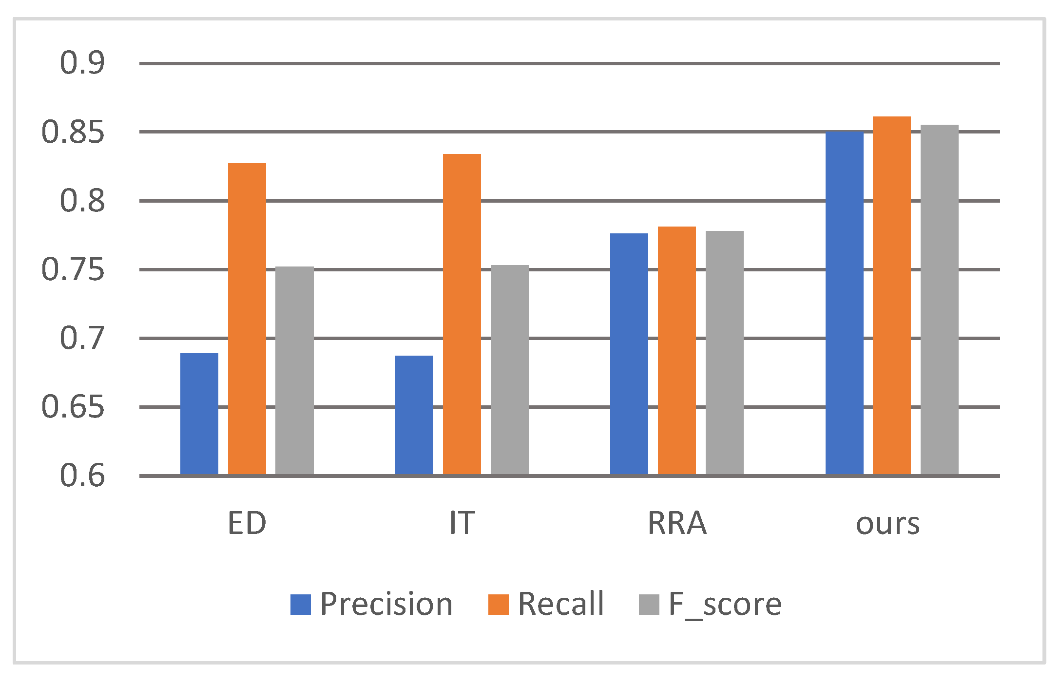


| Methods | Precision | Recall | Fscore | Time/s |
|---|---|---|---|---|
| ED [12] | 0.689 | 0.827 | 0.752 | 0.023 |
| IT [14] | 0.687 | 0.834 | 0.753 | 0.12 |
| RRA [7] | 0.776 | 0.781 | 0.778 | 6.1 |
| Ours | 0.850 | 0.861 | 0.855 | 0.77 |
| RRA | ED | IT | Ours | |
|---|---|---|---|---|
| 0% | 1 | 1 | 1 | 1 |
| 30% | 0.6 | 0.47 | 0.96 | 0.99 |
| 50% | 0.39 | 0.1 | 0.65 | 0.75 |
| 100% | 0.01 | 0 | 0.26 | 0.5 |
| RRA | ED | IT | Ours | |
|---|---|---|---|---|
| 0% | 1 | 1 | 1 | 1 |
| 30% | 0.67 | 0.64 | 0.98 | 0.99 |
| 50% | 0.54 | 0.17 | 0.77 | 0.85 |
| 100% | 0.02 | 0 | 0.4 | 0.67 |
Disclaimer/Publisher’s Note: The statements, opinions and data contained in all publications are solely those of the individual author(s) and contributor(s) and not of MDPI and/or the editor(s). MDPI and/or the editor(s) disclaim responsibility for any injury to people or property resulting from any ideas, methods, instructions or products referred to in the content. |
© 2025 by the authors. Licensee MDPI, Basel, Switzerland. This article is an open access article distributed under the terms and conditions of the Creative Commons Attribution (CC BY) license (https://creativecommons.org/licenses/by/4.0/).
Share and Cite
Han, L.; Zhuang, Y.; Chen, K.; Xie, Y.; Liao, G.; Yin, G.; Lin, J. Circle Detection with Adaptive Parameterization: A Bottom-Up Approach. Sensors 2025, 25, 2552. https://doi.org/10.3390/s25082552
Han L, Zhuang Y, Chen K, Xie Y, Liao G, Yin G, Lin J. Circle Detection with Adaptive Parameterization: A Bottom-Up Approach. Sensors. 2025; 25(8):2552. https://doi.org/10.3390/s25082552
Chicago/Turabian StyleHan, Lin, Yan Zhuang, Ke Chen, Yuhua Xie, Guoliang Liao, Guangfu Yin, and Jiangli Lin. 2025. "Circle Detection with Adaptive Parameterization: A Bottom-Up Approach" Sensors 25, no. 8: 2552. https://doi.org/10.3390/s25082552
APA StyleHan, L., Zhuang, Y., Chen, K., Xie, Y., Liao, G., Yin, G., & Lin, J. (2025). Circle Detection with Adaptive Parameterization: A Bottom-Up Approach. Sensors, 25(8), 2552. https://doi.org/10.3390/s25082552