
Semantic Fusion Algorithm of 2D LiDAR and Camera Based on Contour and Inverse Projection


Abstract
1. Introduction
- (1)
- In contrast to [19,20], whose calibration method relies on special targets and line features, a target-less calibration method based on random environmental targets is proposed in this paper. Two sets of point-line geometric constraints can be derived from a single photo. Circular or elliptical targets are also utilized in the calibration process. The calibration matrix is computed using multiple pairs of point-line constraints, reducing the number of targets required and enhancing adaptability to complex industrial environments. Additionally, the algorithm directly establishes data correspondence between 2D LiDAR and camera images, reducing cumulative error and computational complexity compared to the two-step calibration method.
- (2)
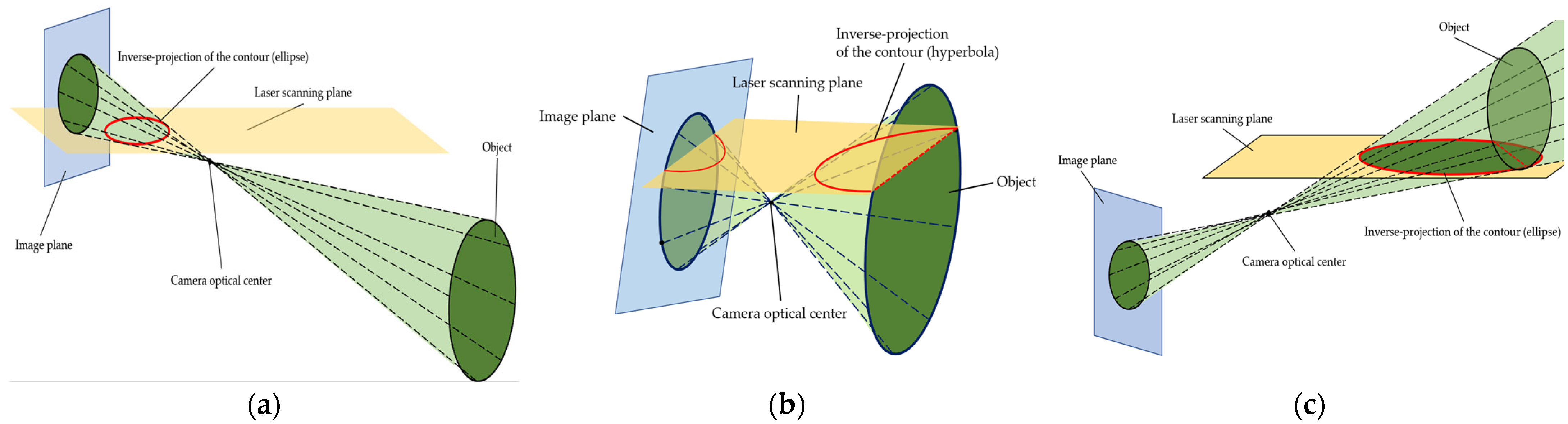
- Different from [21,22], a unique inverse projection curve is obtained by projecting the contour of the target on the image back to the laser scanning plane. Based on the properties of the inverse projection curve, a semantic segmentation algorithm based on the target inverse projection curve is further proposed. The method is specifically designed to be versatile and applicable to both linear features and arc features, which significantly broadens the range of features that can be utilized in various tasks. This flexibility is a key advantage, as it allows the method to adapt to a wider variety of real-world scenarios, where both types of features are commonly encountered. By leveraging this adaptability, our method enhances the performance of calibration and semantic segmentation tasks, enabling more robust and accurate results across different environments and settings. The ability to seamlessly integrate linear and arc features improves the overall applicability of the approach, making it more generalizable and effective for practical use. Compared to existing semantic segmentation methods for LiDAR point clouds, the proposed algorithm requires only one or two projections to filter the laser points that correspond to a specific target, which reduces computational load while enhancing the accuracy of point cloud searches and the speed of establishing semantic targets.
- (3)
- The effectiveness of the proposed semantic fusion algorithm of LiDAR and cameras based on contour and inverse projection is verified by experiments.
2. Related Works
2.1. Calibration of LiDAR and Camera Data
2.2. Semantic Segmentation Algorithm for Laser Point Cloud
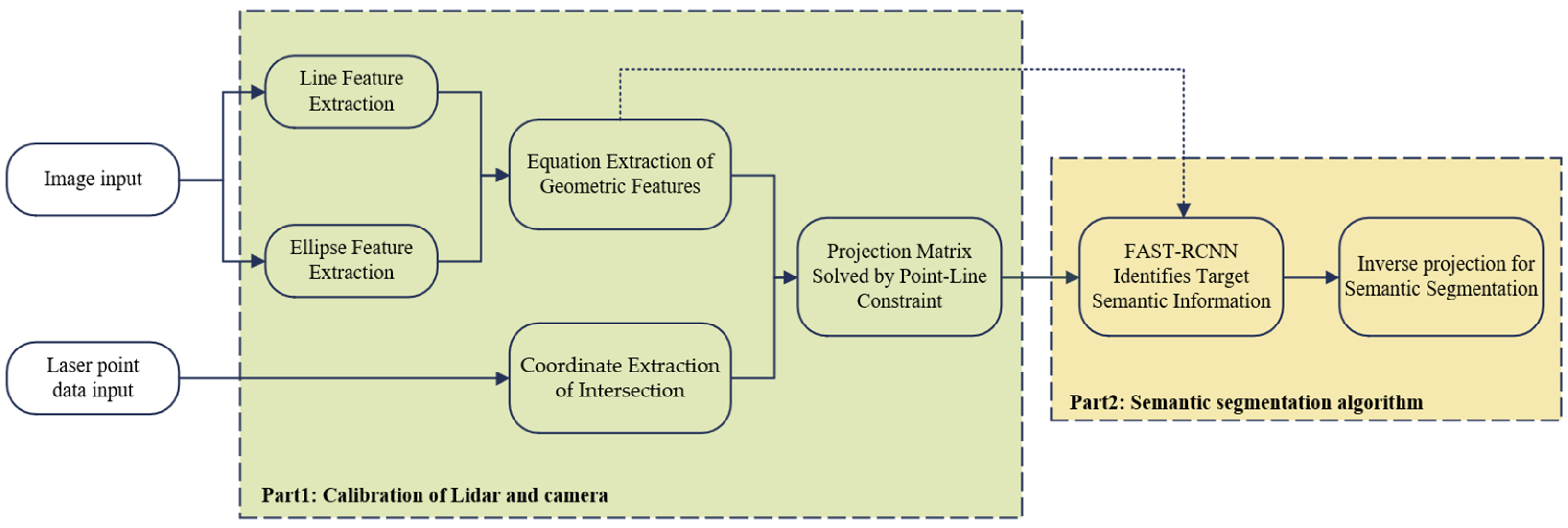
3. Algorithm Framework and Notation
4. Calibration of LiDAR and Camera Data
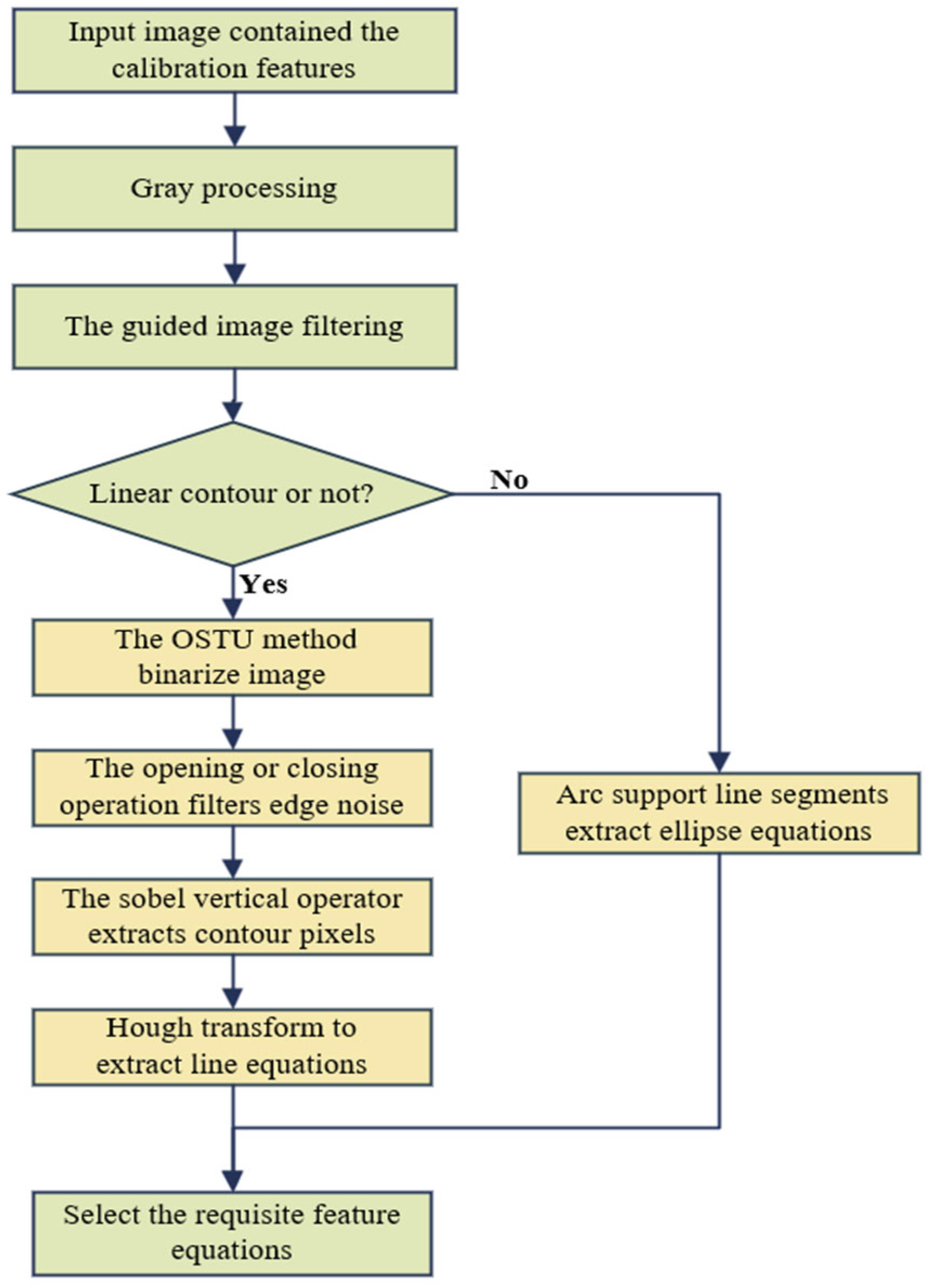
4.1. Image Features Extraction
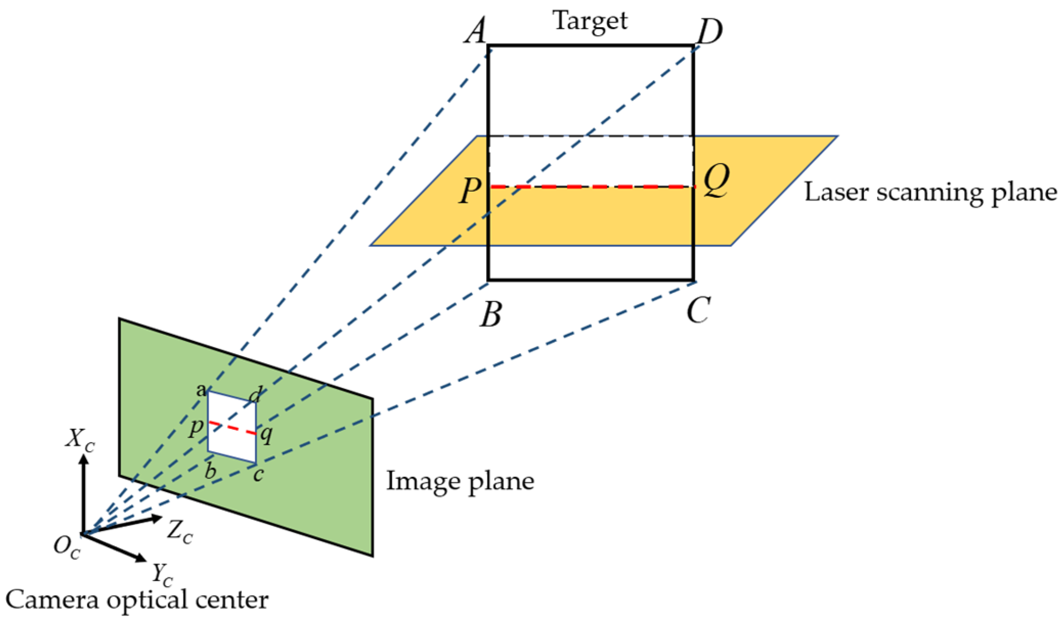
4.2. Coordinate Extraction of Intersection Between Laser Scanning Plane and Target Contour
4.3. Projection Matrix Construction and Solution
5. Semantic Segmentation Algorithm for Laser Point Cloud
5.1. Projective Geometry and Inverse Projection of Contours
5.2. Improved Image Feature Extraction
5.3. Semantic Segmentation Algorithm Based on Contour Inverse Projection
6. Experimental Verification and Analysis
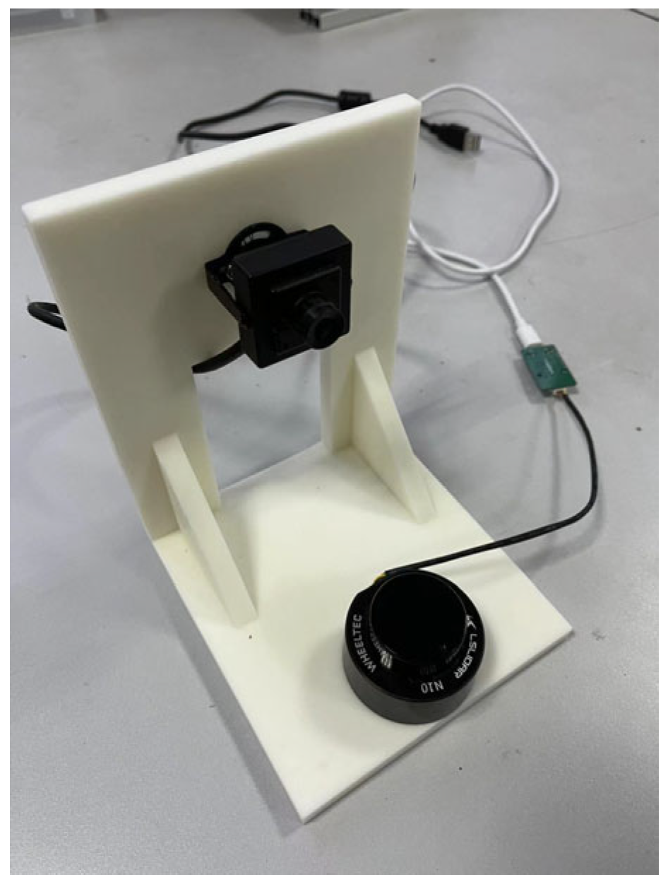
6.1. Experimental Equipment and Environment
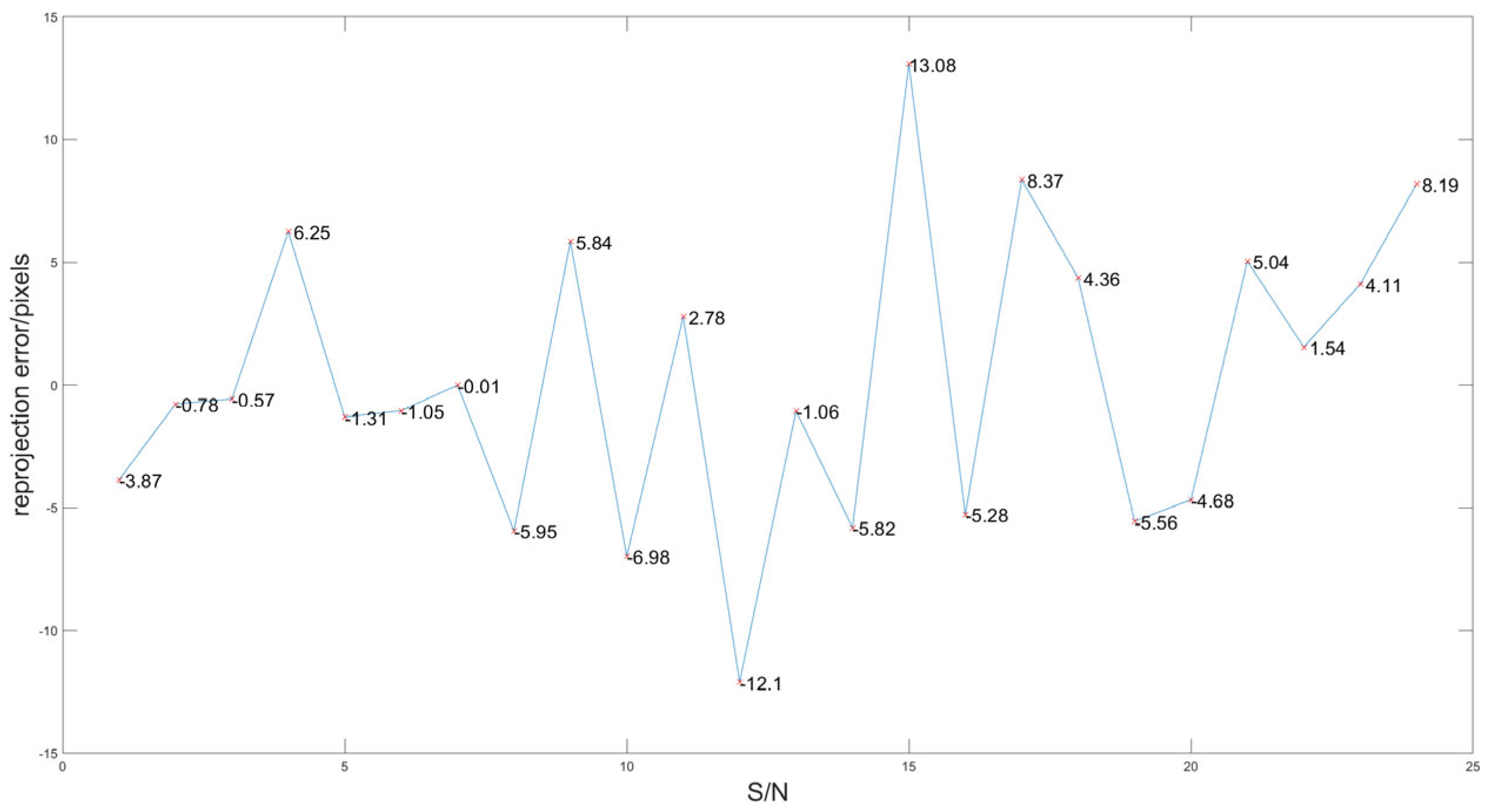
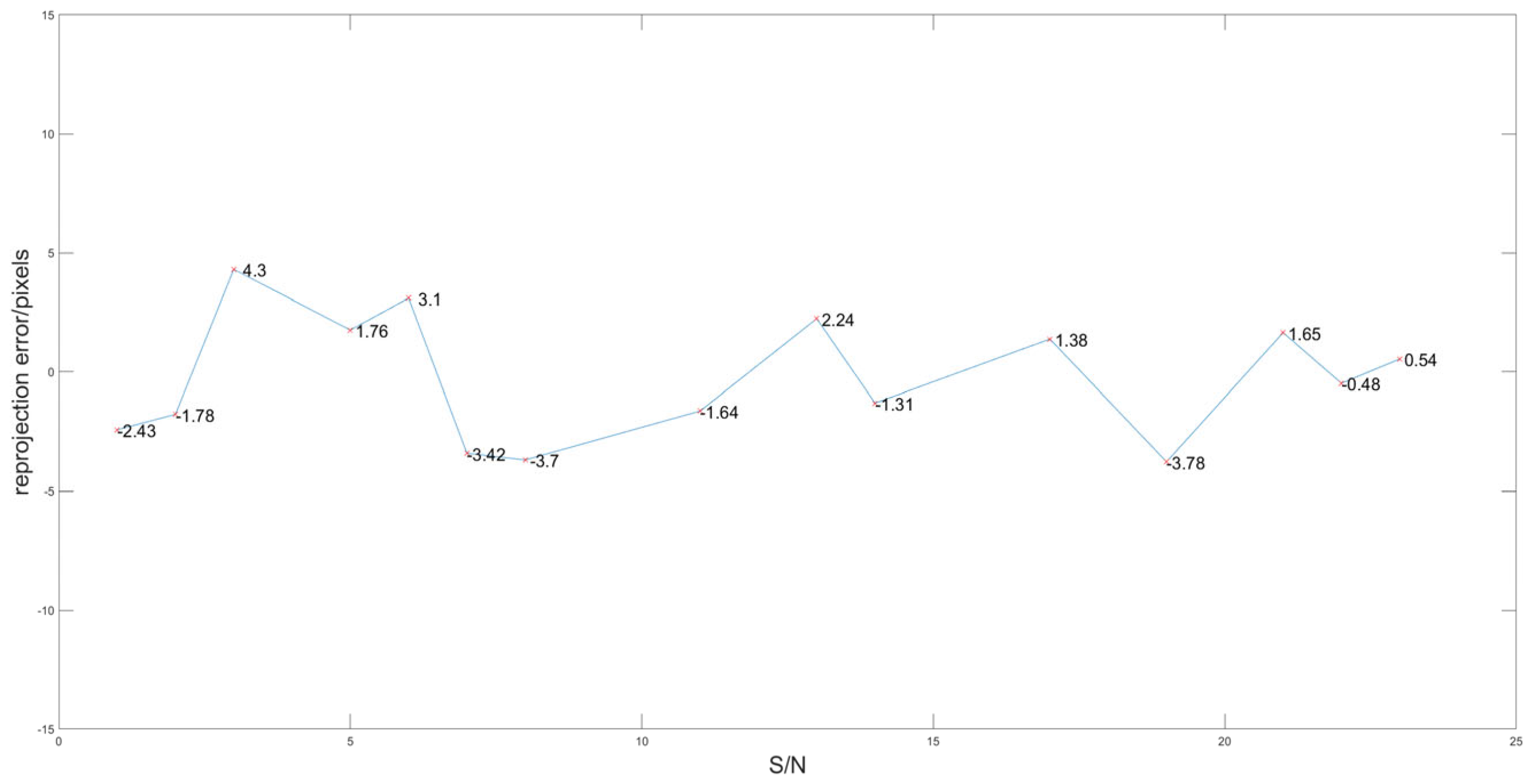
6.2. Experimental Results of Calibration and Analysis
6.3. Comparison with Mainstream Algorithms
Explanation of Methods
6.4. Experimental Results of Semantic Segmentation and Analysis
6.5. Discussion and Future Planning
7. Conclusions
Author Contributions
Funding
Institutional Review Board Statement
Informed Consent Statement
Data Availability Statement
Conflicts of Interest
References
- Meng, J.; Wang, S.; Jiang, L.; Hu, Z.; Xie, Y. Accurate and Efficient Self-Localization of AGV Relying on Trusted Area Information in Dynamic Industrial Scene. IEEE Trans. Veh. Technol. 2023, 72, 7148–7159. [Google Scholar] [CrossRef]
- Zhang, X.; Huang, Y.; Wang, S.; Meng, W.; Li, G.; Xie, Y. Motion planning and tracking control of a four-wheel independently driven steered mobile robot with multiple maneuvering modes. Front. Mech. Eng. 2021, 16, 504–527. [Google Scholar] [CrossRef]
- Jiang, L.; Wang, S.; Xie, Y.; Xie, S.; Zheng, S.; Meng, J.; Ding, H. Decoupled Fractional Supertwisting Stabilization of Interconnected Mobile Robot Under Harsh Terrain Conditions. IEEE Trans. Ind. Electron. 2022, 69, 8178–8189. [Google Scholar] [CrossRef]
- Xie, Y.; Zhang, X.; Zheng, S.; Ahn, C.; Wang, S. Asynchronous H∞ Continuous Stabilization of Mode-Dependent Switched Mobile Robot. IEEE Trans. Syst. Man Cybern. Syst. 2022, 52, 6906–6920. [Google Scholar] [CrossRef]
- Meng, J.; Wan, L.; Wang, S.; Jiang, L.; Li, G.; Wu, L.; Xie, Y. Efficient and Reliable LiDAR-Based Global Localization of Mobile Robots Using Multiscale/Resolution Maps. IEEE Trans. Instrum. Meas. 2021, 70, 1–15. [Google Scholar] [CrossRef]
- Lou, L.; Li, Y.; Zhang, Q.; Wei, H. SLAM and 3D Semantic Reconstruction Based on the Fusion of LiDAR and Monocular Vision. Sensors 2023, 23, 1502. [Google Scholar] [CrossRef] [PubMed]
- Bavle, H.; Sanchez-Lopez, J.L.; Cimarelli, C.; Tourani, A.; Voos, H. From SLAM to Situational Awareness: Challenges and Survey. Sensors 2023, 23, 4849. [Google Scholar] [CrossRef]
- Ghadimzadeh Alamdari, A.; Zade, F.A.; Ebrahimkhanlou, A. A Review of Simultaneous Localization and Mapping for the Robotic-Based Nondestructive Evaluation of Infrastructures. Sensors 2025, 25, 712. [Google Scholar] [CrossRef]
- Tourani, A.; Bavle, H.; Sanchez-Lopez, J.L.; Voos, H. Visual SLAM: What Are the Current Trends and What to Expect? Sensors 2022, 22, 9297. [Google Scholar] [CrossRef]
- Zou, Q.; Sun, Q.; Chen, L.; Nie, B.; Li, Q. A Comparative Analysis of LiDAR SLAM-Based Indoor Navigation for Autonomous Vehicles. IEEE Trans. Intell. Transp. Syst. 2022, 23, 6907–6921. [Google Scholar] [CrossRef]
- An, Y.; Shi, J.; Gu, D.; Liu, Q. Visual-LiDAR SLAM Based on Unsupervised Multi-channel Deep Neural Networks. Cogn. Comput. 2022, 14, 1496–1508. [Google Scholar] [CrossRef]
- Zhang, Q.; Pless, R. Extrinsic calibration of a camera and laser range finder (improves camera calibration). In Proceedings of the IEEE/RSJ International Conference on Intelligent Robots and Systems, Sendai, Japan, 28 September–2 October 2004; pp. 2301–2306. [Google Scholar]
- Li, Y.; Ruichek, Y.; Cappelle, C. Optimal Extrinsic Calibration Between a Stereoscopic System and a LIDAR. IEEE Trans. Instrum. Meas. 2013, 62, 2258–2269. [Google Scholar] [CrossRef]
- Peng, G.; Zhou, Y.; Hu, L.; Xiao, L.; Sun, Z.; Wu, Z.; Zhu, X. VILO SLAM: Tightly Coupled Binocular Vision–Inertia SLAM Combined with LiDAR. Sensors 2023, 23, 4588. [Google Scholar] [CrossRef] [PubMed]
- Kim, T.; Kang, M.; Kang, S.; Kim, D. Improvement of Door Recognition Algorithm using LiDAR and RGB-D camera for Mobile Manipulator. In Proceedings of the 2022 IEEE Sensors Applications Symposium (SAS), Sundsvall, Sweden, 1–3 August 2022; pp. 1–6. [Google Scholar]
- Pang, L.; Cao, Z.; Yu, J.; Liang, S.; Chen, X.; Zhang, W. An Efficient 3D Pedestrian Detector with Calibrated RGB Camera and 3D LiDAR. In Proceedings of the 2019 IEEE International Conference on Robotics and Biomimetics (ROBIO), Dali, China, 6–8 December 2019; pp. 2902–2907. [Google Scholar]
- Xiang, Z.; Yu, J.; Li, J.; Su, J. ViLiVO: Virtual LiDAR-Visual Odometry for an Autonomous Vehicle with a Multi-Camera System. In Proceedings of the 2019 IEEE/RSJ International Conference on Intelligent Robots and Systems (IROS), Macau, China, 3–8 November 2019; pp. 2486–2492. [Google Scholar]
- Girshick, R. Fast R-CNN. In Proceedings of the 2015 IEEE International Conference on Computer Vision (ICCV), Santiago, Chile, 7–13 December 2015; pp. 1440–1448. [Google Scholar]
- Itami, F.; Yamazaki, T. A Simple Calibration Procedure for a 2D LiDAR With Respect to a Camera. IEEE Sens. J. 2019, 19, 7553–7564. [Google Scholar] [CrossRef]
- Zhou, L.; Deng, Z. A new algorithm for the establishing data association between a camera and a 2-D LIDAR. Tsinghua Sci. Technol. 2014, 19, 314–322. [Google Scholar] [CrossRef]
- Qi, X.; Wang, W.; Liao, Z.; Zhang, X.; Yang, D.; Wei, R. Object Semantic Grid Mapping with 2D LiDAR and RGB-D Camera for Domestic Robot Navigation. Appl. Sci. 2020, 10, 5782. [Google Scholar] [CrossRef]
- Lai, X.; Yuan, Y.; Li, Y.; Wang, M. Full-Waveform LiDAR Point Clouds Classification Based on Wavelet Support Vector Machine and Ensemble Learning. Sensors 2019, 19, 3191. [Google Scholar] [CrossRef]
- Mirzaei, F.M.; Kottas, D.G.; Roumeliotis, S.I. 3D LIDAR–camera intrinsic and extrinsic calibration: Identifiability and analytical least-squares-based initialization. Int. J. Robot. Res. 2012, 31, 452–467. [Google Scholar] [CrossRef]
- Peng, M.; Wan, Q.; Chen, B.; Wu, S. A Calibration Method of 2D LiDAR and a Camera Based on Effective Lower Bound Estimation of Observation Probability. J. Electron. Inf. Technol. 2022, 44, 2478–2487. [Google Scholar]
- Itami, F.; Yamazaki, T. An improved method for the calibration of a 2-D LiDAR with respect to a camera by using a checkerboard target. IEEE Sens. J. 2020, 2, 7906–7917. [Google Scholar] [CrossRef]
- Petek, K.; Vödisch, N.; Meyer, J.; Cattaneo, D.; Valada, A.; Burgard, W. Automatic Target-Less Camera-LiDAR Calibration From Motion and Deep Point Correspondences. IEEE Robot. Autom. Lett. 2024, 9, 9978–9985. [Google Scholar] [CrossRef]
- Koide, K.; Oishi, S.; Yokozuka, M.; Banno, A. General, Single-shot, Target-less, and Automatic LiDAR-Camera Extrinsic Calibration Toolbox. In Proceedings of the 2023 IEEE International Conference on Robotics and Automation (ICRA), London, UK, 29 May–2 June 2023. [Google Scholar]
- Yang, H.; Liu, X.; Patras, I. A simple and effective extrinsic calibration method of a camera and a single line scanning LiDAR. In Proceedings of the 21st International Conference on Pattern Recognition, Tsukuba, Japan, 11–15 November 2012; pp. 1439–1442. [Google Scholar]
- Briales, J.; Gonzalez-Jimenez, J. A minimal solution for the calibration of a 2D laser-rangefinder and a camera based on scene corners. In Proceedings of the IEEE/RSJ International Conference on Intelligent Robots and Systems, Hamburg, Germany, 28 September–2 October 2015; pp. 1891–1896. [Google Scholar]
- Zhang, L.; Xu, X.; He, J.; Zhu, K.; Luo, Z.; Tan, Z. Calibration Method of 2D LIDAR and Camera Based on Indoor Structural Features. Acta Photonica Sin. 2020, 49, 1214001. [Google Scholar]
- Shrihari, V.; Stefan, G.; Viet, N.; Roland, S. Cognitive maps for mobile robots an object-based approach. Robot. Auton. Syst. 2007, 55, 359–371. [Google Scholar]
- Song, L.; Min, W.; Zhou, L.; Wang, Q.; Zhao, H. Vehicle Logo Recognition Using Spatial Structure Correlation and YOLO-T. Sensors 2023, 23, 4313. [Google Scholar] [CrossRef] [PubMed]
- Liu, W.; Angurlov, D.; Erhan, D.; Szegedy, C.; Reed, S.; Cheng-Yang, F.; Berg, A. SSD: Single Shot MultiBox Detector. Eur. Conf. Comput. Vis. 2016, 9905, 21–37. [Google Scholar]
- Lee, T.; Kim, C.; Cho, D. A Monocular Vision Sensor-Based Efficient SLAM Method for Indoor Service Robots. IEEE Trans. Ind. Electron. 2019, 66, 318–328. [Google Scholar] [CrossRef]
- Liang, J.; Qiao, Y.; Guan, T.; Manocha, D. OF-VO: Efficient Navigation Among Pedestrians Using Commodity Sensors. IEEE Robot. Autom. Lett. 2021, 6, 6148–6155. [Google Scholar] [CrossRef]
- Li, J.; Stevenson, R. 2D LiDAR and Camera Fusion Using Motion Cues for Indoor Layout Estimation. In Proceedings of the 2021 IEEE 24th International Conference on Information Fusion (FUSION), Sun City, South Africa, 1–4 November 2021; pp. 1–6. [Google Scholar]
- Verucchi, M.; Bartoli, L.; Bagni, F.; Gatti, F.; Burgio, P.; Bertogna, M. Real-Time clustering and LiDAR-camera fusion on embedded platforms for self-driving cars. In Proceedings of the 2020 Fourth IEEE International Conference on Robotic Computing (IRC), Taichung, Taiwan, 9–11 November 2020; pp. 398–405. [Google Scholar]
- Shahian Jahromi, B.; Tulabandhula, T.; Cetin, S. Real-Time Hybrid Multi-Sensor Fusion Framework for Perception in Autonomous Vehicles. Sensors 2019, 19, 4357. [Google Scholar] [CrossRef]
- Ostu, N. A threshold selection method from gray-level histograms. IEEE Trans. Syst. Man Cybern. 1979, 9, 62–66. [Google Scholar]
- Grompone von Gioi, R.; Jakubowicz, J.; Morel, J.; Randall, G. LSD: A Fast Line Segment Detector with a False Detection Control. IEEE Trans. Pattern Anal. Mach. Intell. 2010, 32, 722–732. [Google Scholar] [CrossRef]
- Lu, C.; Xia, S.; Shao, M.; Fu, Y. Arc-Support Line Segments Revisited: An Efficient High-Quality Ellipse Detection. IEEE Trans. Image Process. 2020, 29, 768–781. [Google Scholar] [CrossRef] [PubMed]
- Hartley, R.; Zisserman, A. Multiple View Geometry in Computer Vision; Cambridge University Press: Cambridge, UK, 2003. [Google Scholar]


| S/N | a | b | c | ||
|---|---|---|---|---|---|
| 1 | 0.6077 | 1.3984 | 0.9945 | 0.1045 | −816 |
| 0.1446 | 1.5715 | 0.9998 | 0.0175 | −468 | |
| 2 | 0.6678 | 1.1350 | 0.7314 | −0.6820 | −464 |
| 0.2112 | 1.2595 | 0.7071 | 0.7071 | −581 | |
| 3 | 0.6021 | 1.1178 | 0.8988 | −0.4384 | −654 |
| 0.1839 | 1.2626 | 0.4540 | 0.8910 | −495 | |
| 4 | 0.3736 | 1.0628 | 0.6947 | −0.7193 | −275 |
| −0.1396 | 1.2232 | 0.7431 | 0.6691 | −374 | |
| 5 | 0.4913 | 0.7056 | 1 | 0 | −987 |
| 0.0182 | 0.8574 | 0.9998 | −0.0175 | −385 | |
| 6 | 0.9665 | 1.4957 | 0.9205 | 0.3907 | −987 |
| 0.4754 | 1.7439 | 0.9135 | 0.4067 | −707 | |
| 7 | 0.7442 | 0.6956 | 0.8829 | 0.4695 | −1263 |
| 0.2333 | 0.8803 | 0.9135 | 0.4067 | −718 | |
| 8 | 0.3107 | 1.5084 | 0.9994 | −0.0349 | −555 |
| −0.1861 | 1.6463 | 0.9986 | −0.0523 | −223 | |
| 9 | 0.4115 | 0.6749 | 0.8910 | −0.4540 | −654 |
| −0.1470 | 0.8026 | 0.5000 | 0.8660 | −371 | |
| 10 | 0.6974 | 0.8088 | 0.9336 | −0.3584 | −924 |
| 0.2475 | 1.1092 | 0.9397 | −0.3420 | −459 | |
| 11 | 0.6062 | 1.7807 | 0.8480 | 0.5299 | −733 |
| 0.0517 | 1.9347 | 0.8572 | 0.5150 | −468 | |
| 12 | 0.2098 | 1.3290 | 0.4067 | −0.9135 | 50 |
| −0.1505 | 1.3549 | 0.9063 | 0.4226 | −324 |
| S/N | |||
|---|---|---|---|
| 1 | 0.6477 | 0.5456 | |
| 0.2180 | 0.7751 | ||
| 2 | 0.3871 | 0.8617 | |
| −0.1031 | 0.8991 | ||
| 3 | 0.9402 | 0.9984 | |
| 0.5272 | 1.2396 | ||
| 4 | 0.6753 | 1.1803 | |
| 0.2088 | 1.3124 | ||
| 5 | 0.7494 | 1.4319 | |
| 0.3896 | 1.6011 | ||
| 6 | 1.0446 | 1.0482 | |
| 0.6917 | 1.3522 |
| Method | Description | Key Feature | Advantages | Disadvantages |
|---|---|---|---|---|
| Method [25] | Utilizes predefined calibration targets to align LiDAR and camera data (‘target-based’) | Checkerboard | High precision in controlled environments | Requires manual setup of targets, potential cumulative errors |
| Method [30] | Employs indoor structural features for calibration without predefined targets (“target-less”) | Line features | Adaptive to feature regular environments | Less precise in feature-sparse areas |
| Ours | Utilizes a variety of environmental morphological features for calibration and precision optimization (“target-less”) | Line features and arc features | High adaptability and precision in diverse environments; Improved feature utilization | Less effectiveness in high-speed dynamic areas |
| Method [25] | Method [30] | Ours | |
|---|---|---|---|
| Average reprojection error/pixels | 6.54 | 4.88 | 2.78 |
| Error distribution interval/pixels | [4.13, 9.64] | [1.55, 6.20] | [1.49, 5.78] |
| Method [25] | Method [30] | Ours | |
|---|---|---|---|
| Calibration time/s | 0.82 | 0.85 | 1.03 |
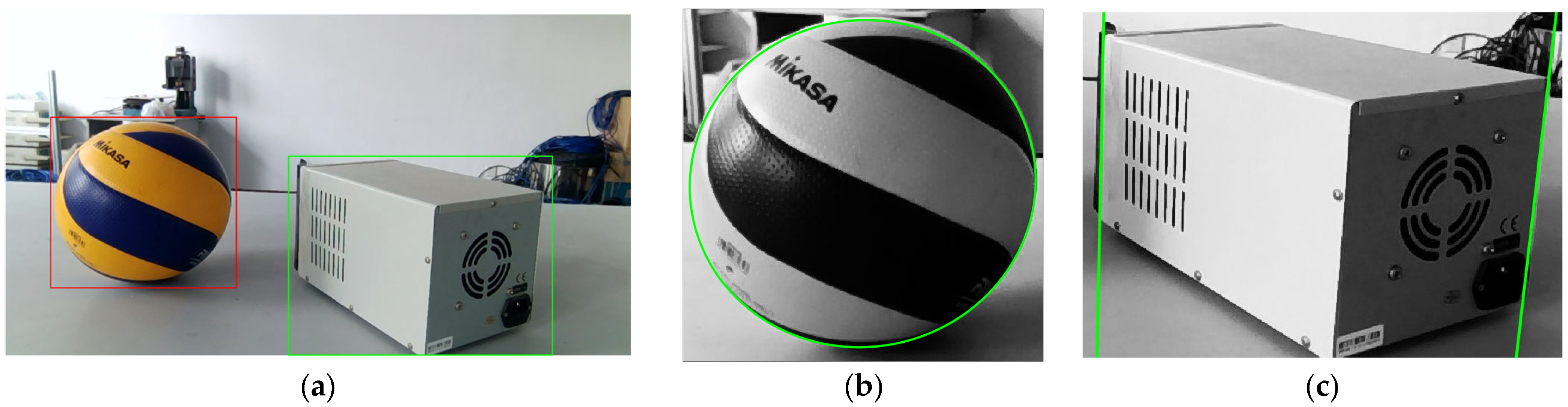
| Object | Color |
|---|---|
| ball | red |
| instruments | green |
Disclaimer/Publisher’s Note: The statements, opinions and data contained in all publications are solely those of the individual author(s) and contributor(s) and not of MDPI and/or the editor(s). MDPI and/or the editor(s) disclaim responsibility for any injury to people or property resulting from any ideas, methods, instructions or products referred to in the content. |
© 2025 by the authors. Licensee MDPI, Basel, Switzerland. This article is an open access article distributed under the terms and conditions of the Creative Commons Attribution (CC BY) license (https://creativecommons.org/licenses/by/4.0/).
Share and Cite
Yuan, X.; Liu, Y.; Xiong, T.; Zeng, W.; Wang, C. Semantic Fusion Algorithm of 2D LiDAR and Camera Based on Contour and Inverse Projection. Sensors 2025, 25, 2526. https://doi.org/10.3390/s25082526
Yuan X, Liu Y, Xiong T, Zeng W, Wang C. Semantic Fusion Algorithm of 2D LiDAR and Camera Based on Contour and Inverse Projection. Sensors. 2025; 25(8):2526. https://doi.org/10.3390/s25082526
Chicago/Turabian StyleYuan, Xingyu, Yu Liu, Tifan Xiong, Wei Zeng, and Chao Wang. 2025. "Semantic Fusion Algorithm of 2D LiDAR and Camera Based on Contour and Inverse Projection" Sensors 25, no. 8: 2526. https://doi.org/10.3390/s25082526
APA StyleYuan, X., Liu, Y., Xiong, T., Zeng, W., & Wang, C. (2025). Semantic Fusion Algorithm of 2D LiDAR and Camera Based on Contour and Inverse Projection. Sensors, 25(8), 2526. https://doi.org/10.3390/s25082526