
Enhancing Bottleneck Concept Learning in Image Classification


Abstract
1. Introduction
2. Related Works
2.1. Explainable AI
2.2. Concept-Based Framework for Interpretability
2.3. Contrastive Learning
3. Model
3.1. Preliminary
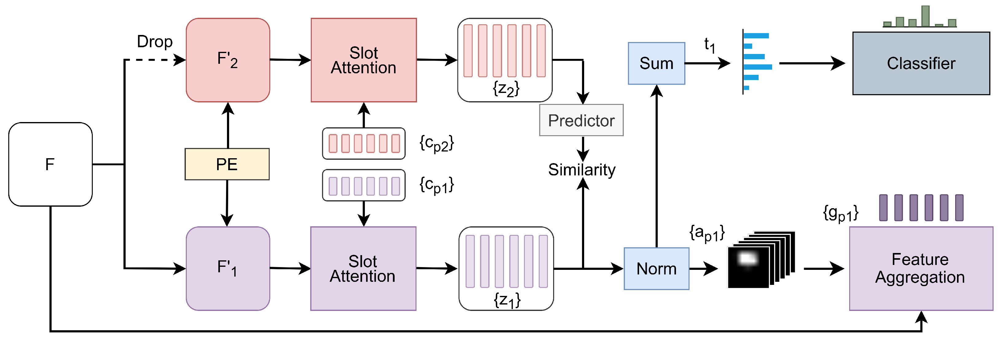
3.2. E-BotCL
3.3. Contrastive Concept Extractor
3.4. Slot-Based Feature Aggregation
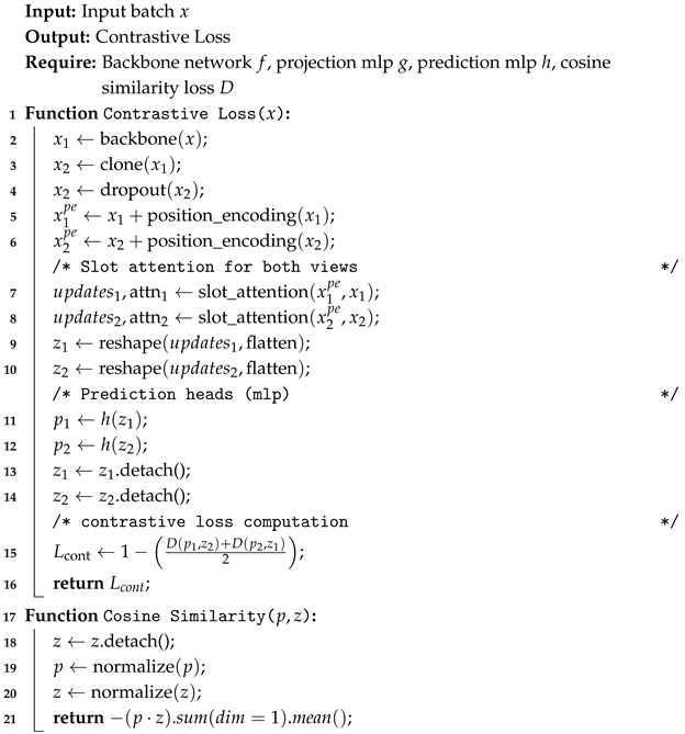
3.5. E-BotCL Loss
| Algorithm 1: Contrastive Loss Pseudocode, PyTorch-like |
 |
4. Results
4.1. Experimental Settings
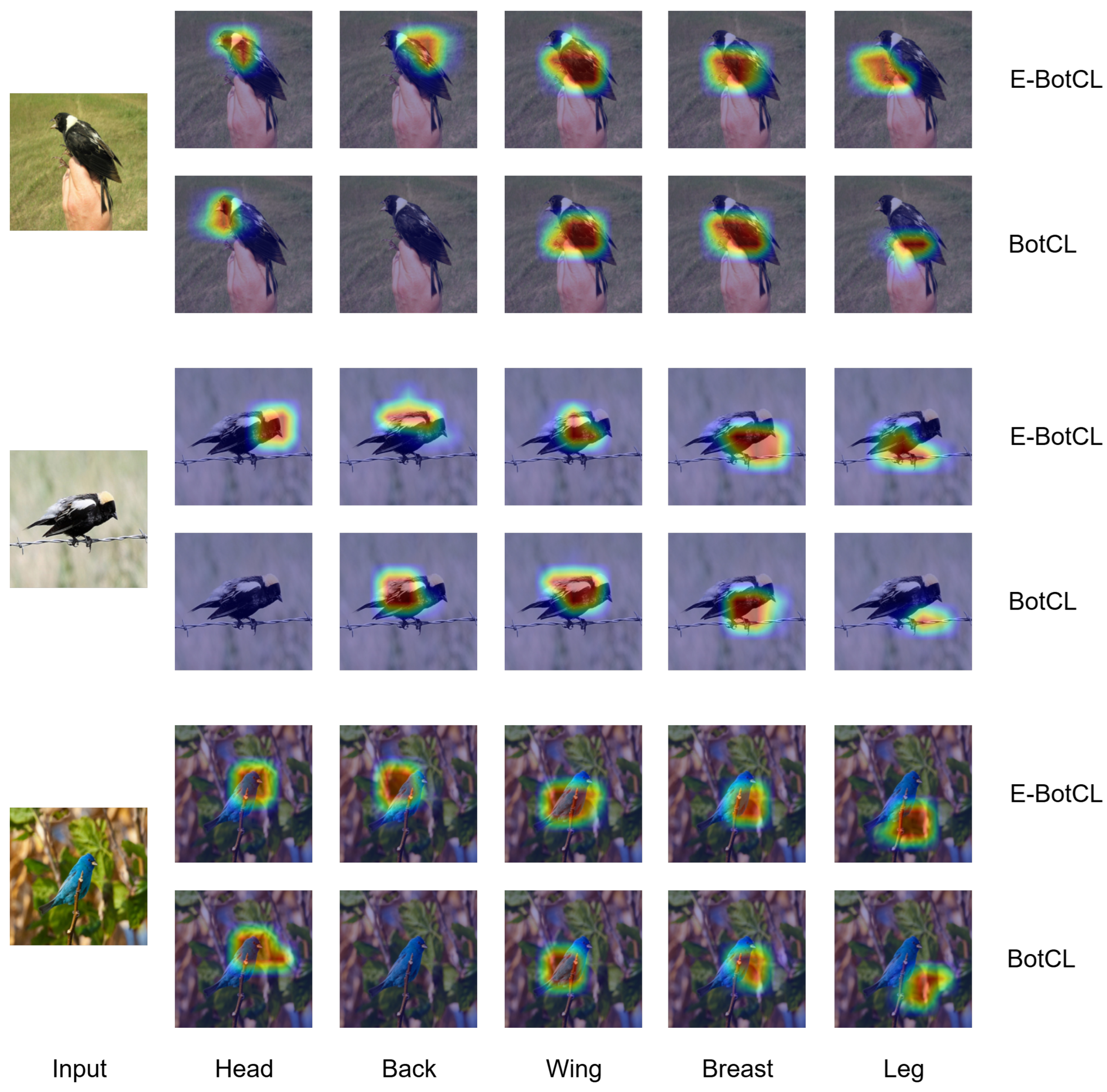
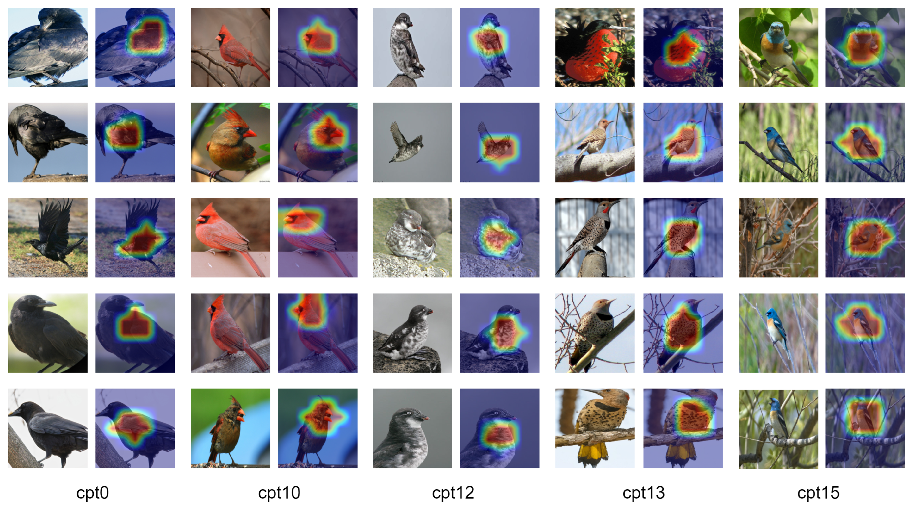
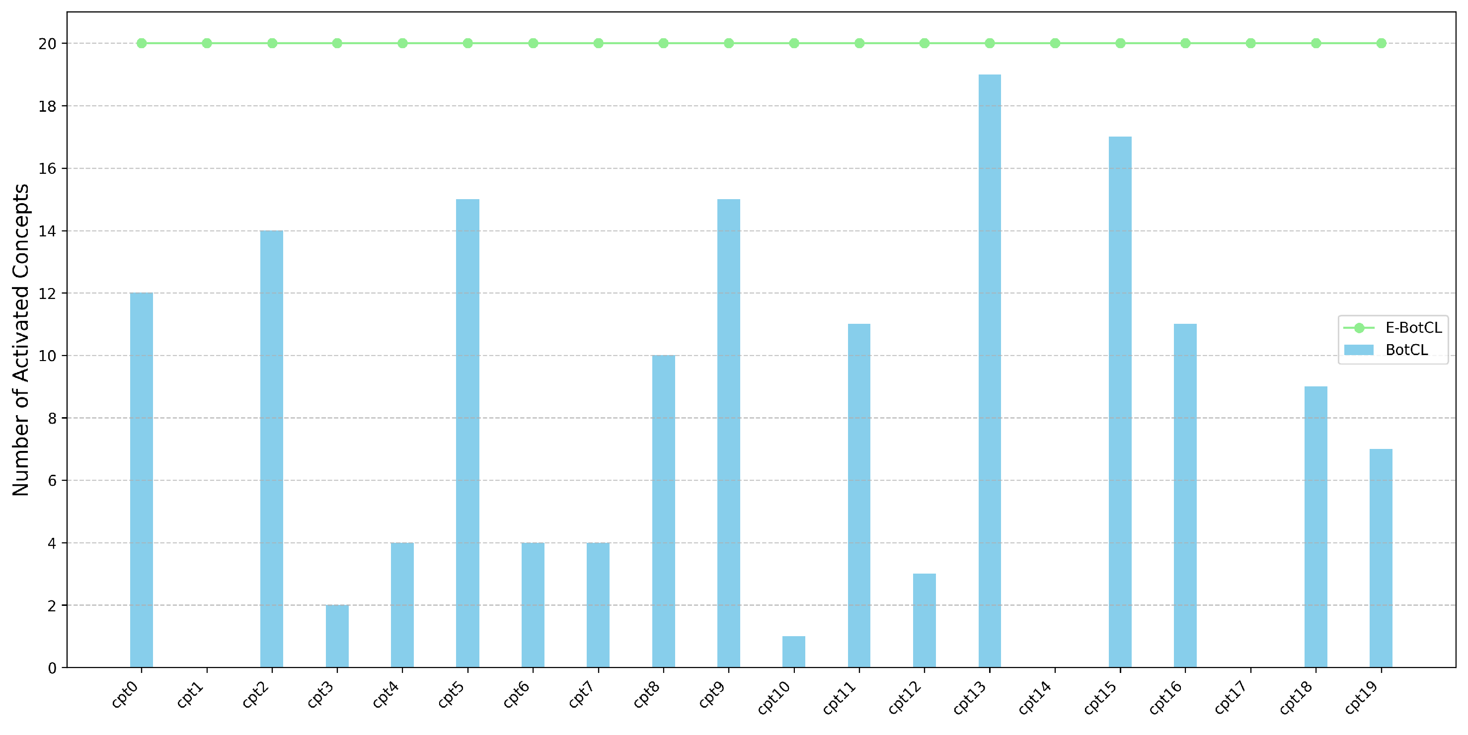
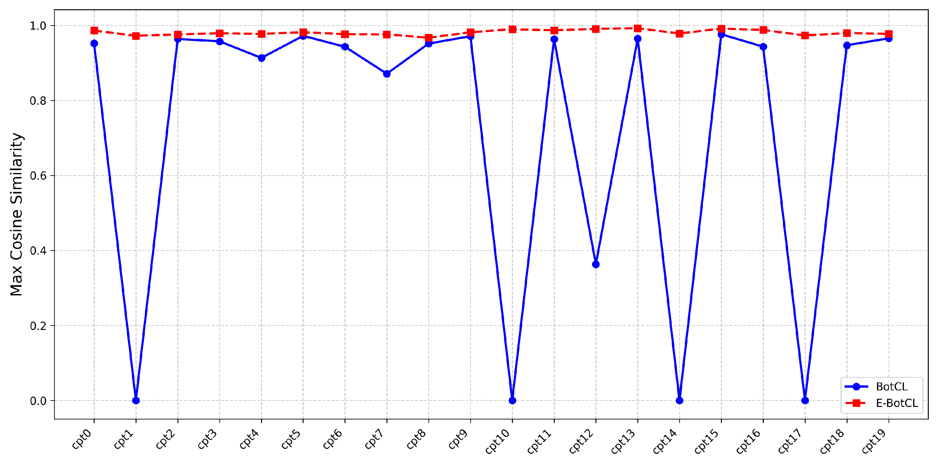
4.2. Interpretability
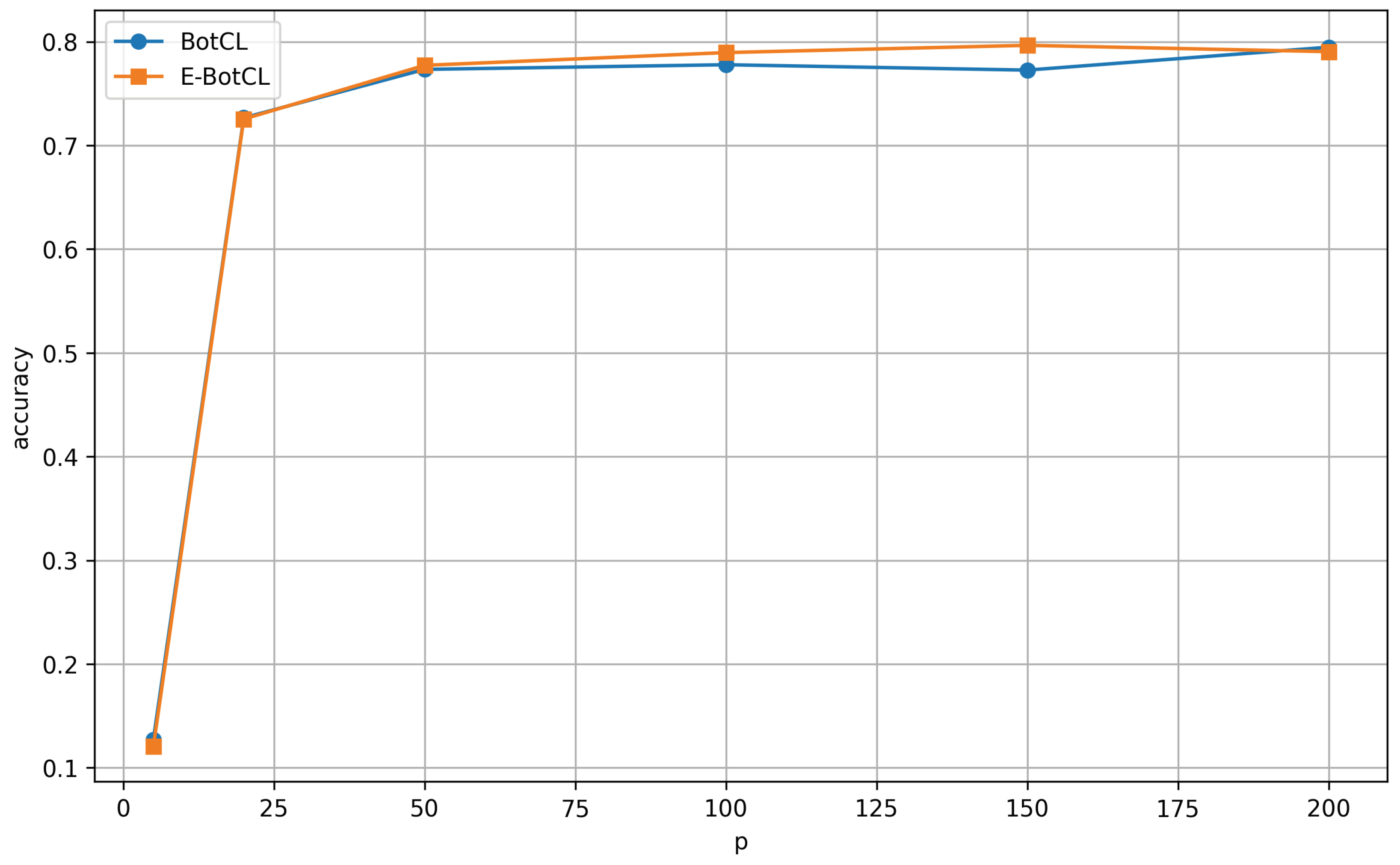
4.3. Classification Performance
4.4. User Study
4.5. Ablation Study
5. Conclusions
Author Contributions
Funding
Institutional Review Board Statement
Informed Consent Statement
Data Availability Statement
Conflicts of Interest
References
- Chen, Y.W.; Jain, L.C. Deep learning in healthcare. In Paradigms and Applications; Springer: Berlin/Heidelberg, Germany, 2020. [Google Scholar]
- Zablocki, É.; Ben-Younes, H.; Pérez, P.; Cord, M. Explainability of deep vision-based autonomous driving systems: Review and challenges. Int. J. Comput. Vis. 2022, 130, 2425–2452. [Google Scholar] [CrossRef]
- Ribeiro, M.T.; Singh, S.; Guestrin, C. “Why should i trust you?” Explaining the predictions of any classifier. In Proceedings of the 22nd ACM SIGKDD International Conference on Knowledge Discovery and Data Mining, San Francisco, CA, USA, 13–17 August 2016; pp. 1135–1144. [Google Scholar]
- Caruana, R.; Lou, Y.; Gehrke, J.; Koch, P.; Sturm, M.; Elhadad, N. Intelligible models for healthcare: Predicting pneumonia risk and hospital 30-day readmission. In Proceedings of the 21th ACM SIGKDD International Conference on Knowledge Discovery and Data Mining, Sydney, Australia, 10–13 August 2015; pp. 1721–1730. [Google Scholar]
- Chattopadhay, A.; Sarkar, A.; Howlader, P.; Balasubramanian, V.N. Grad-cam++: Generalized gradient-based visual explanations for deep convolutional networks. In Proceedings of the 2018 IEEE Winter Conference on Applications of Computer Vision (WACV), Lake Tahoe, NV, USA, 12–15 March 2018; pp. 839–847. [Google Scholar]
- Bach, S.; Binder, A.; Montavon, G.; Klauschen, F.; Müller, K.R.; Samek, W. On pixel-wise explanations for non-linear classifier decisions by layer-wise relevance propagation. PLoS ONE 2015, 10, e0130140. [Google Scholar] [CrossRef] [PubMed]
- Arrieta, A.B.; Díaz-Rodríguez, N.; Del Ser, J.; Bennetot, A.; Tabik, S.; Barbado, A.; García, S.; Gil-López, S.; Molina, D.; Benjamins, R.; et al. Explainable Artificial Intelligence (XAI): Concepts, taxonomies, opportunities and challenges toward responsible AI. Inf. Fusion 2020, 58, 82–115. [Google Scholar] [CrossRef]
- Simonyan, K.; Vedaldi, A.; Zisserman, A. Deep inside convolutional networks: Visualising image classification models and saliency maps. arXiv 2013, arXiv:1312.6034. [Google Scholar]
- Selvaraju, R.R.; Cogswell, M.; Das, A.; Vedantam, R.; Parikh, D.; Batra, D. Grad-CAM: Visual explanations from deep networks via gradient-based localization. Int. J. Comput. Vis. 2020, 128, 336–359. [Google Scholar] [CrossRef]
- Sundararajan, M.; Taly, A.; Yan, Q. Axiomatic attribution for deep networks. In Proceedings of the International Conference on Machine Learning, Sydney, Australia, 6–11 August 2017; pp. 3319–3328. [Google Scholar]
- Poeta, E.; Ciravegna, G.; Pastor, E.; Cerquitelli, T.; Baralis, E. Concept-based explainable artificial intelligence: A survey. arXiv 2023, arXiv:2312.12936. [Google Scholar]
- Wang, B.; Li, L.; Nakashima, Y.; Nagahara, H. Learning bottleneck concepts in image classification. In Proceedings of the IEEE/CVF Conference on Computer Vision and Pattern Recognition, Vancouver, BC, Canada, 17–24 June 2023; pp. 10962–10971. [Google Scholar]
- Fong, R.; Patrick, M.; Vedaldi, A. Understanding deep networks via extremal perturbations and smooth masks. In Proceedings of the IEEE/CVF International Conference on Computer Vision, Seoul, Republic of Korea, 27 October–2 November 2019; pp. 2950–2958. [Google Scholar]
- Shrikumar, A.; Greenside, P.; Kundaje, A. Learning important features through propagating activation differences. In Proceedings of the International Conference on Machine Learning, Sydney, Australia, 6–11 August 2017; pp. 3145–3153. [Google Scholar]
- Wang, B.; Li, L.; Verma, M.; Nakashima, Y.; Kawasaki, R.; Nagahara, H. MTUNet: Few-shot image classification with visual explanations. In Proceedings of the IEEE/CVF Conference on Computer Vision and Pattern Recognition, Nashville, TN, USA, 19–25 June 2021; pp. 2294–2298. [Google Scholar]
- Yeh, C.K.; Kim, B.; Arik, S.; Li, C.L.; Pfister, T.; Ravikumar, P. On completeness-aware concept-based explanations in deep neural networks. Adv. Neural Inf. Process. Syst. 2020, 33, 20554–20565. [Google Scholar]
- Ras, G.; Xie, N.; Van Gerven, M.; Doran, D. Explainable deep learning: A field guide for the uninitiated. J. Artif. Intell. Res. 2022, 73, 329–396. [Google Scholar] [CrossRef]
- Lundberg, S. A unified approach to interpreting model predictions. arXiv 2017, arXiv:1705.07874. [Google Scholar]
- Samek, W. Explainable artificial intelligence: Understanding, visualizing and interpreting deep learning models. arXiv 2017, arXiv:1708.08296. [Google Scholar]
- Akhtar, N. A survey of explainable ai in deep visual modeling: Methods and metrics. arXiv 2023, arXiv:2301.13445. [Google Scholar]
- Rudin, C.; Chen, C.; Chen, Z.; Huang, H.; Semenova, L.; Zhong, C. Interpretable machine learning: Fundamental principles and 10 grand challenges. Stat. Surv. 2022, 16, 1–85. [Google Scholar] [CrossRef]
- Carvalho, D.V.; Pereira, E.M.; Cardoso, J.S. Machine learning interpretability: A survey on methods and metrics. Electronics 2019, 8, 832. [Google Scholar] [CrossRef]
- Nesvijevskaia, A.; Ouillade, S.; Guilmin, P.; Zucker, J.D. The accuracy versus interpretability trade-off in fraud detection model. Data Policy 2021, 3, e12. [Google Scholar] [CrossRef]
- Koh, P.W.; Nguyen, T.; Tang, Y.S.; Mussmann, S.; Pierson, E.; Kim, B.; Liang, P. Concept bottleneck models. In Proceedings of the International Conference on Machine Learning, Virtual Event, 13–18 July 2020; pp. 5338–5348. [Google Scholar]
- Alvarez Melis, D.; Jaakkola, T. Towards robust interpretability with self-explaining neural networks. Adv. Neural Inf. Process. Syst. 2018, 31. [Google Scholar]
- Ge, Y.; Xiao, Y.; Xu, Z.; Zheng, M.; Karanam, S.; Chen, T.; Itti, L.; Wu, Z. A peek into the reasoning of neural networks: Interpreting with structural visual concepts. In Proceedings of the IEEE/CVF Conference on Computer Vision and Pattern Recognition, Nashville, TN, USA, 19–25 June 2021; pp. 2195–2204. [Google Scholar]
- Ghorbani, A.; Wexler, J.; Zou, J.Y.; Kim, B. Towards automatic concept-based explanations. Adv. Neural Inf. Process. Syst. 2019, 32. [Google Scholar]
- Laugel, T.; Lesot, M.J.; Marsala, C.; Renard, X.; Detyniecki, M. The dangers of post-hoc interpretability: Unjustified counterfactual explanations. arXiv 2019, arXiv:1907.09294. [Google Scholar]
- Zhang, R.; Isola, P.; Efros, A.A.; Shechtman, E.; Wang, O. The unreasonable effectiveness of deep features as a perceptual metric. In Proceedings of the IEEE Conference on Computer Vision and Pattern Recognition, Salt Lake City, UT, USA, 18–22 June 2018; pp. 586–595. [Google Scholar]
- Chen, X.; Fan, H.; Girshick, R.; He, K. Improved baselines with momentum contrastive learning. arXiv 2020, arXiv:2003.04297. [Google Scholar]
- He, K.; Fan, H.; Wu, Y.; Xie, S.; Girshick, R. Momentum contrast for unsupervised visual representation learning. In Proceedings of the IEEE/CVF Conference on Computer Vision and Pattern Recognition, Seattle, WA, USA, 14–19 June 2020; pp. 9729–9738. [Google Scholar]
- Chen, X.; He, K. Exploring simple siamese representation learning. In Proceedings of the IEEE/CVF Conference on Computer Vision and Pattern Recognition, Nashville, TN, USA, 19–25 June 2021; pp. 15750–15758. [Google Scholar]
- Grill, J.B.; Strub, F.; Altché, F.; Tallec, C.; Richemond, P.; Buchatskaya, E.; Doersch, C.; Avila Pires, B.; Guo, Z.; Gheshlaghi Azar, M.; et al. Bootstrap your own latent-a new approach to self-supervised learning. Adv. Neural Inf. Process. Syst. 2020, 33, 21271–21284. [Google Scholar]
- Fong, R.C.; Vedaldi, A. Interpretable explanations of black boxes by meaningful perturbation. In Proceedings of the IEEE International Conference on Computer Vision, Venice, Italy, 22–29 October 2017; pp. 3429–3437. [Google Scholar]
- He, K.; Gkioxari, G.; Dollár, P.; Girshick, R. Mask r-cnn. In Proceedings of the IEEE International Conference on Computer Vision, Venice, Italy, 22–29 October 2017; pp. 2961–2969. [Google Scholar]
- Redmon, J. Yolov3: An incremental improvement. arXiv 2018, arXiv:1804.02767. [Google Scholar]
- Li, L.; Wang, B.; Verma, M.; Nakashima, Y.; Kawasaki, R.; Nagahara, H. Scouter: Slot attention-based classifier for explainable image recognition. In Proceedings of the IEEE/CVF International Conference on Computer Vision, Montreal, BC, Canada, 11–17 October 2021; pp. 1046–1055. [Google Scholar]
- Locatello, F.; Weissenborn, D.; Unterthiner, T.; Mahendran, A.; Heigold, G.; Uszkoreit, J.; Dosovitskiy, A.; Kipf, T. Object-centric learning with slot attention. Adv. Neural Inf. Process. Syst. 2020, 33, 11525–11538. [Google Scholar]
- Welinder, P.; Branson, S.; Mita, T.; Wah, C.; Schroff, F.; Belongie, S.; Perona, P. Caltech-UCSD Birds 200; Technical Report CNS-TR-2010-001; California Institute of Technology: Pasadena, CA, USA, 2010. [Google Scholar]
- Deng, J.; Dong, W.; Socher, R.; Li, L.J.; Li, K.; Fei-Fei, L. Imagenet: A large-scale hierarchical image database. In Proceedings of the 2009 IEEE Conference on Computer Vision and Pattern Recognition, Miami, FL, USA, 20–25 June 2009; pp. 248–255. [Google Scholar]
- He, K.; Zhang, X.; Ren, S.; Sun, J. Deep residual learning for image recognition. In Proceedings of the IEEE Conference on Computer Vision and Pattern Recognition, Las Vegas, NV, USA, 27–30 June 2016; pp. 770–778. [Google Scholar]
- Chen, C.; Li, O.; Tao, D.; Barnett, A.; Rudin, C.; Su, J.K. This looks like that: Deep learning for interpretable image recognition. Adv. Neural Inf. Process. Syst. 2019, 32. [Google Scholar]


| CUB200 | ImageNet | |
|---|---|---|
| k-means [16] | 0.063 | 0.427 |
| PCA [16] | 0.044 | 0.139 |
| SENN [25] | 0.642 | 0.673 |
| ProtoPNet [42] | 0.725 | 0.752 |
| BotCL | 0.725 | 0.768 |
| E-BotCL | 0.726 | 0.770 |
| CDR (↑) | CC (↑) | MIC (↓) | ||||
|---|---|---|---|---|---|---|
| Mean | Std | Mean | Std | Mean | Std | |
| BotCL | 0.3896 | 0.4527 | 0.2466 | 0.3361 | 0.2489 | 0.0787 |
| E-BotCL | 1.0000 | 0.0000 | 0.6952 | 0.1396 | 0.1706 | 0.0512 |
| BotCL | CL | MTL | Acc | #Params | Training Time | GPU Memory |
|---|---|---|---|---|---|---|
| ✓ | 0.7733 | 14.37 M | 65 min | 6.8 GB | ||
| ✓ | ✓ | 0.7758 | 15.61 M | 83 min | 7.1 GB | |
| ✓ | ✓ | 0.7765 | 16.10 M | 96 min | 9.3 GB | |
| ✓ | ✓ | ✓ | 0.7772 | 17.34 M | 107 min | 9.6 GB |
Disclaimer/Publisher’s Note: The statements, opinions and data contained in all publications are solely those of the individual author(s) and contributor(s) and not of MDPI and/or the editor(s). MDPI and/or the editor(s) disclaim responsibility for any injury to people or property resulting from any ideas, methods, instructions or products referred to in the content. |
© 2025 by the authors. Licensee MDPI, Basel, Switzerland. This article is an open access article distributed under the terms and conditions of the Creative Commons Attribution (CC BY) license (https://creativecommons.org/licenses/by/4.0/).
Share and Cite
Cheng, X.; Niu, Z.; Jiang, Z.; Li, L. Enhancing Bottleneck Concept Learning in Image Classification. Sensors 2025, 25, 2398. https://doi.org/10.3390/s25082398
Cheng X, Niu Z, Jiang Z, Li L. Enhancing Bottleneck Concept Learning in Image Classification. Sensors. 2025; 25(8):2398. https://doi.org/10.3390/s25082398
Chicago/Turabian StyleCheng, Xingfu, Zhaofeng Niu, Zhouqiang Jiang, and Liangzhi Li. 2025. "Enhancing Bottleneck Concept Learning in Image Classification" Sensors 25, no. 8: 2398. https://doi.org/10.3390/s25082398
APA StyleCheng, X., Niu, Z., Jiang, Z., & Li, L. (2025). Enhancing Bottleneck Concept Learning in Image Classification. Sensors, 25(8), 2398. https://doi.org/10.3390/s25082398