Resource-Constrained Specific Emitter Identification Based on Efficient Design and Network Compression


Abstract
1. Introduction
1.1. Background
1.2. Motivations
1.3. Related Works
1.4. Main Contributions
- We propose a lightweight convolution network, LCNet. The implementation of strategies such as complex convolution, depth-wise separable convolution, and attention mechanisms can enhance model performance while reducing complexity.
- We introduce a sparse feature selection (SFS) framework for RC-SEI. Specifically, the incorporation of scaling factors and corresponding sparse regularization in the FC layer enable effective model compression.
- Based on the effectiveness of the RC-SEI method proposed in this paper, we suggest a standardized procedure for designing lightweight network models.
2. System Model and Problem Formulation
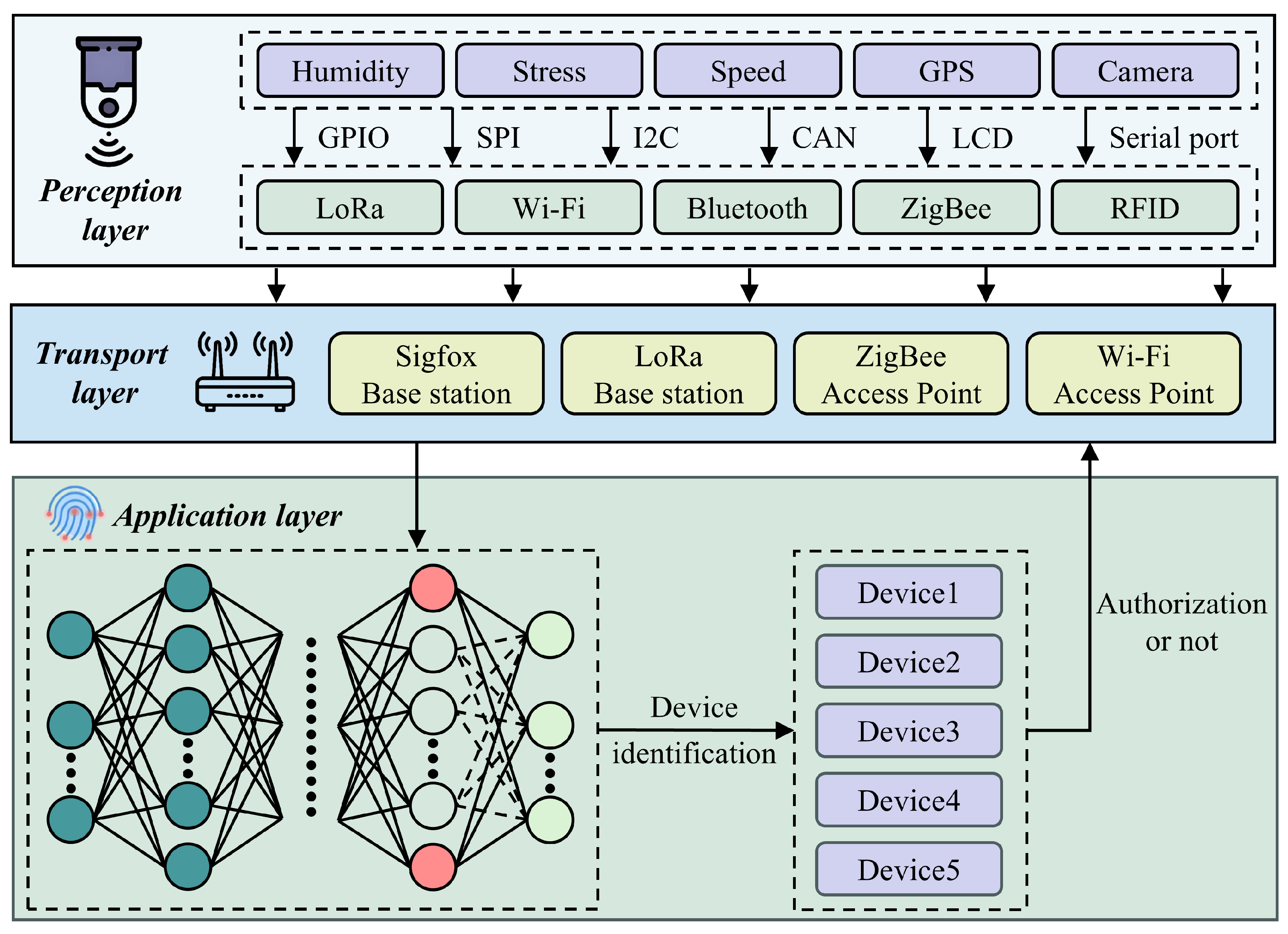
2.1. System Model
2.2. Problem Formulation
2.2.1. SEI Problem
2.2.2. RC-SEI Problem
3. The Proposed RC-SEI Method
3.1. Lightweight Convolution Network Architecture
3.1.1. IQCF
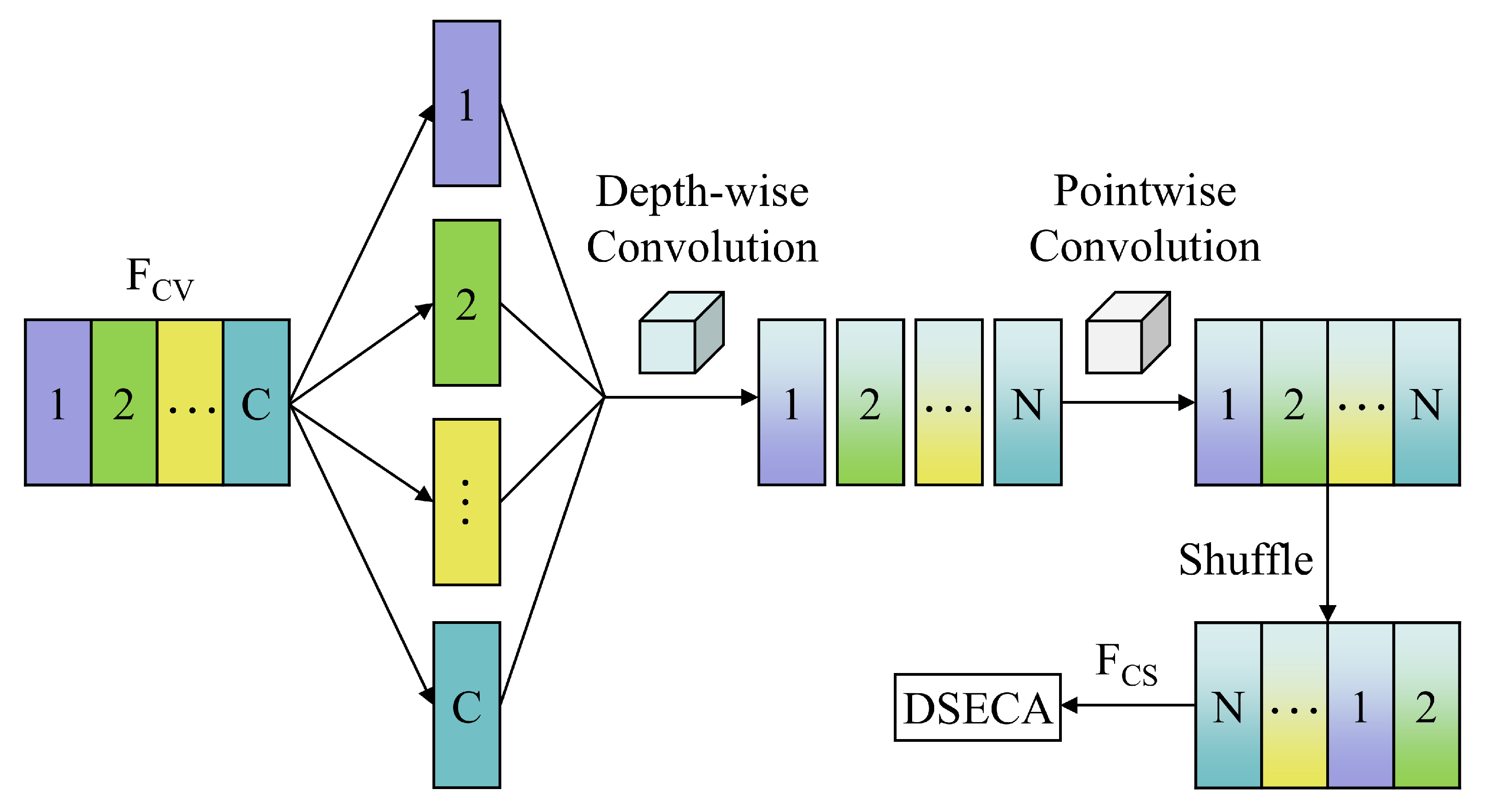
3.1.2. LCM
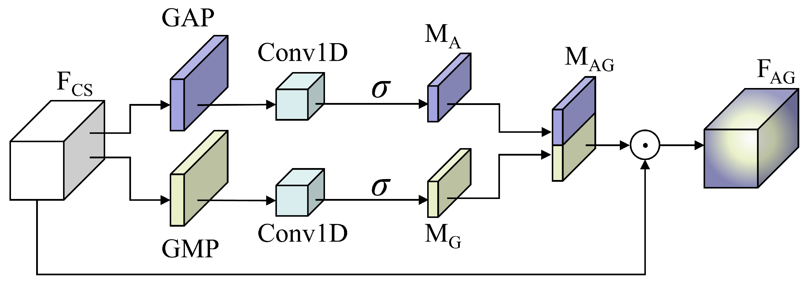
3.1.3. DSECA
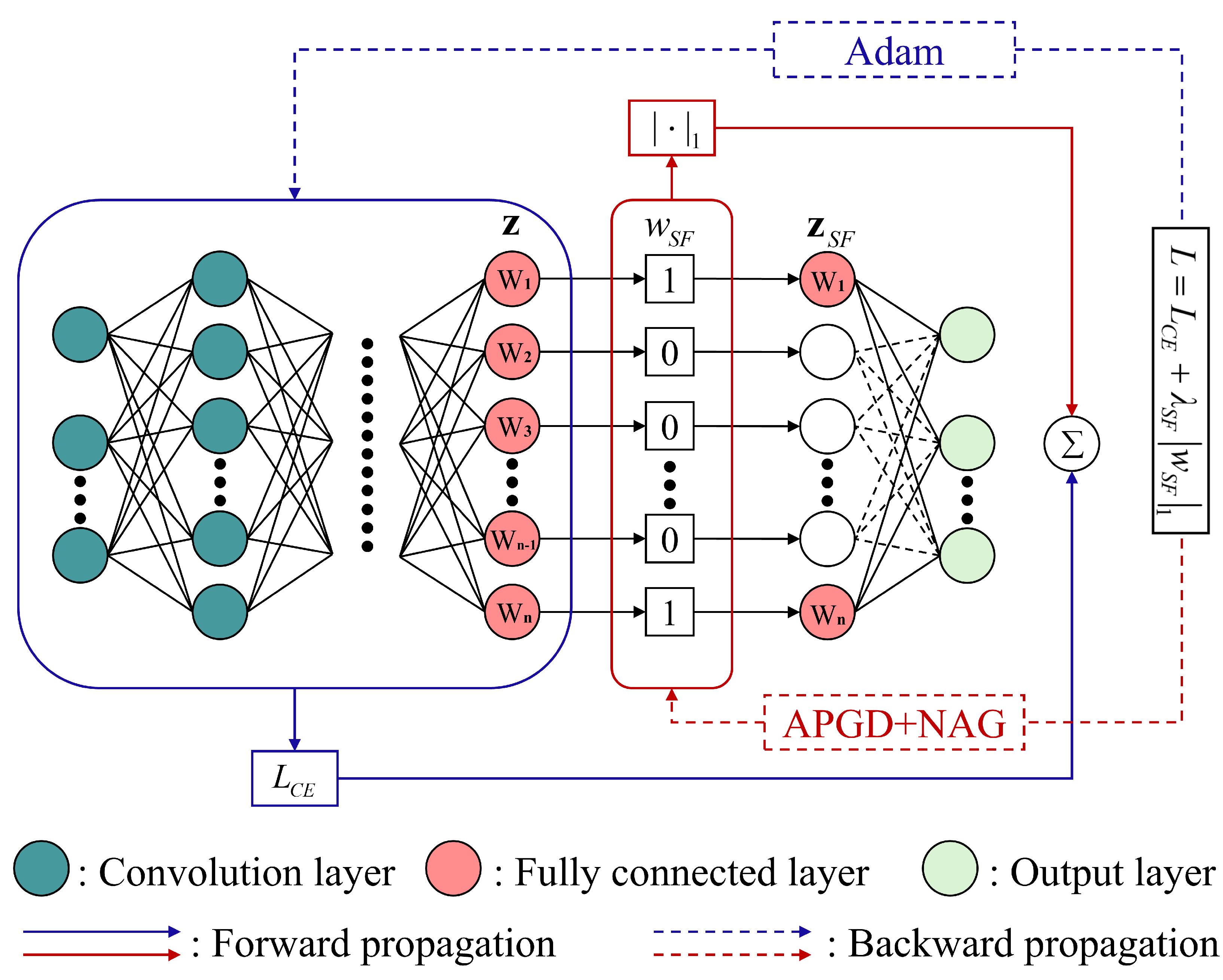
3.2. Sparse Feature Selection
3.3. APGD-NAG Optimization Algorithm and Training Procedure
| Algorithm 1: Training Procedure of the RC-SEI method. |
Require:
|
4. Experimental Setup and Results
4.1. Experimental Methodology
4.1.1. Datasets
4.1.2. Baseline Models
4.2. LCNet Evaluation
4.2.1. LCNet vs. StdNet
4.2.2. Ablation Study
4.3. SFS Framework Evalution
4.3.1. Sparse Factor Impact
4.3.2. Retraining Efficacy
4.3.3. Comparative Network Analysis
- Effectiveness: The SFS framework can be readily applied to both high-precision and lightweight models, with the compressed models largely maintaining comparable accuracy levels to their uncompressed counterparts. Specifically, in accuracy tests on two datasets, MCNet experienced only a 0.90% decrease in accuracy on the ADS-B dataset, whereas CVNN saw decreases of 0.20% and 0.45% on the ADS-B and Wi-Fi datasets, respectively. The accuracy of other models either remained consistent or exhibited an improvement in post-compression performance. Notably, our proposed LCNet achieved the advanced level of accuracy on both datasets, with performance levels of 99.40% and 99.90%, respectively.
- Limitations: The effectiveness of model compression methods based on the SFS framework is contingent on the model’s complexity. For highly complex models, the parameter compression rate tends to be lower. However, the employment of efficiently designed ULCNN and our proposed LCNet can yield superior parameter compression results.
- Extension: It is noteworthy that SFS can compress over 99% of the parameters and FLOPs in the FC layer. Consequently, the parameter compression rates and FLOPs reductions shown in Table 8 accurately reflect the proportion of complexity within the FC layer relative to the overall model complexity. This indicates that there is a significant amount of redundancy in network models beyond the FC layer. To minimize overall model redundancy, building upon the RC-SEI method proposed in this paper, we suggest designing lightweight network models following these steps:
- Initially, a high-performance neural network model should be trained without regard for complexity.
- Subsequently, utilizing the dark knowledge from the initial step and efficient network design principles, redesign a compact neural network model.
- Finally, applying the SFS framework to massively compress the complexity of the FC layer.
4.3.4. Complexity Analysis
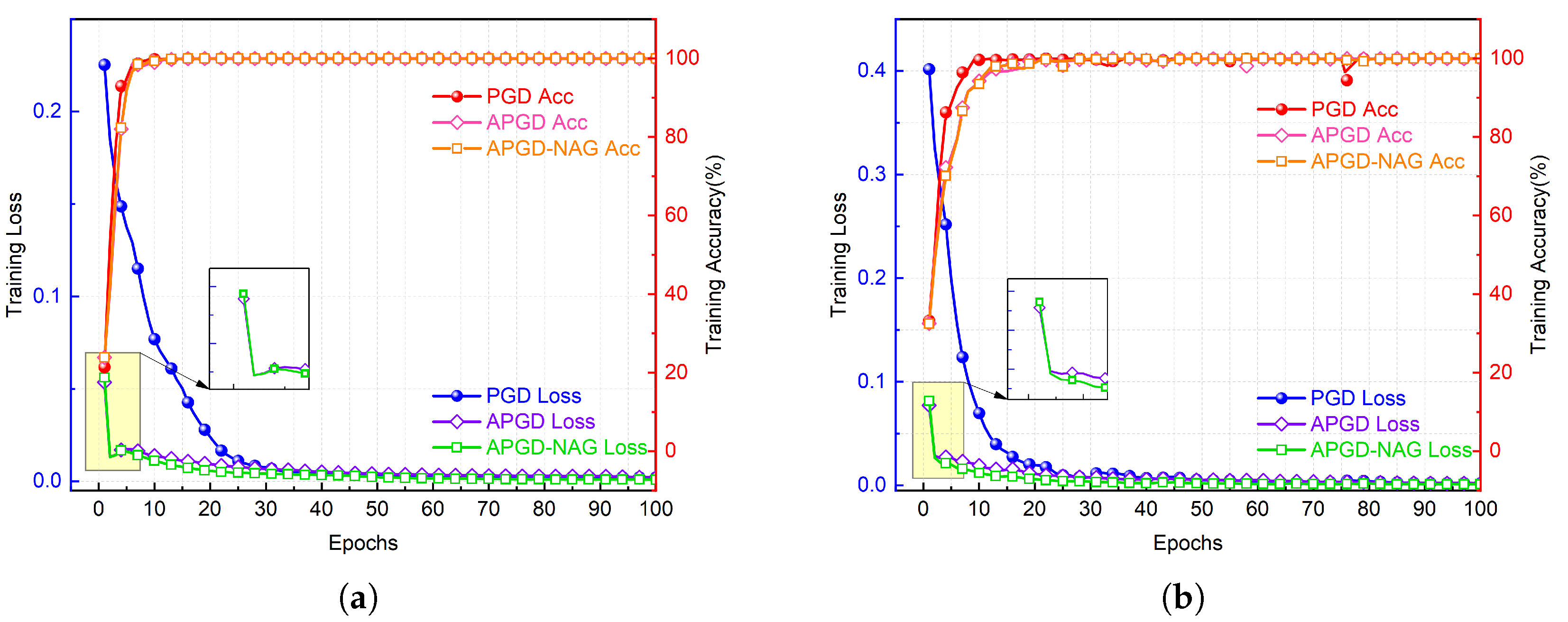
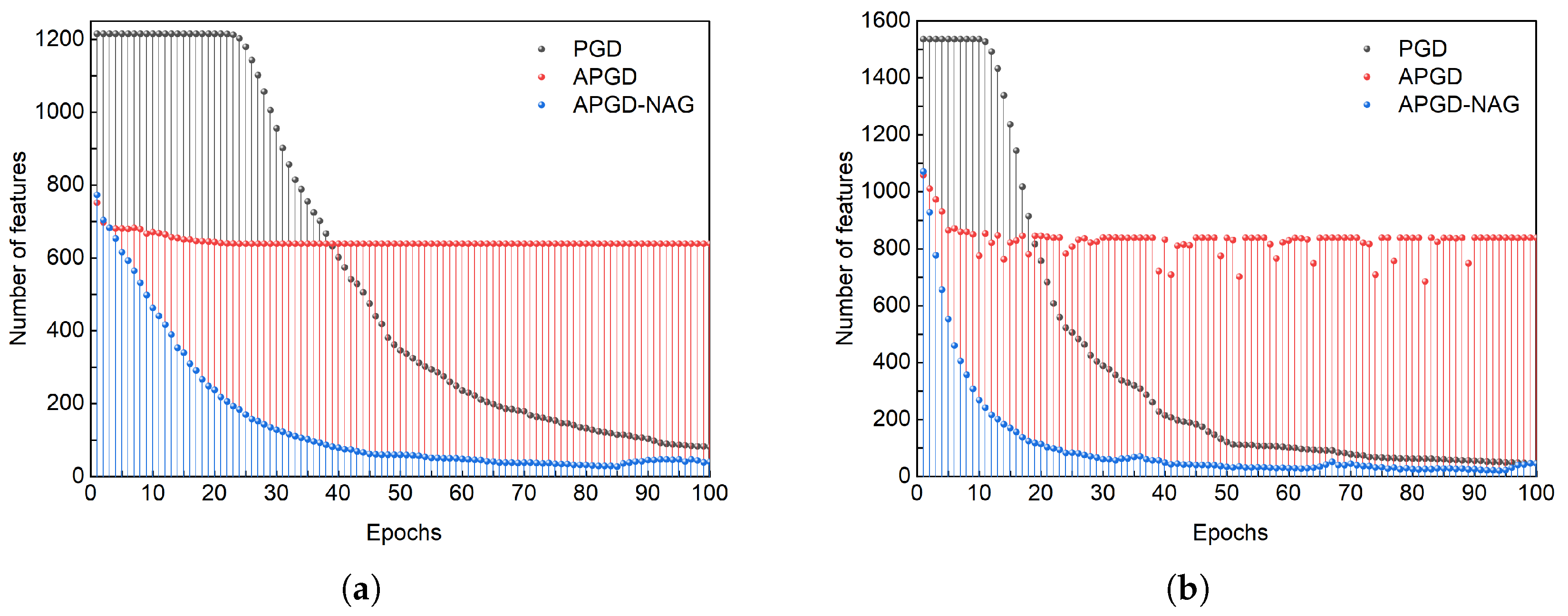
4.4. APGD-NAG Evaluation
5. Conclusions
Author Contributions
Funding
Institutional Review Board Statement
Informed Consent Statement
Data Availability Statement
Conflicts of Interest
References
- Rajora, R.; Rajora, A.; Sharma, B.; Aggarwal, P.; Thapliyal, S. Sensing the Future: Challenges and Trends in IoT Sensor Technology. In Proceedings of the 4th International Conference on Innovative Practices in Technology and Management, ICIPTM, Greater Noida, India, 23–25 February 2024; pp. 1–5. [Google Scholar]
- Chakrabarty, R.; Karmakar, R.; Das, N.K.; Shivam, S.; Mondal, I. The Future of Real-Time Remote Monitoring: The Role of Low-Cost IoT Sensor Systems. In Proceedings of the 7th International Conference on Electronics, Materials Engineering & Nano-Technology (IEMENTech), Kolkata, India, 5–7 July 2023; pp. 1–5. [Google Scholar]
- Yin, X.; Wang, S.; Shahzad, M.; Hu, J. An IoT-Oriented Privacy-Preserving Fingerprint Authentication System. IEEE Internet Things J. 2021, 9, 11760–11771. [Google Scholar] [CrossRef]
- Sun, P.; Shen, S.; Wan, Y.; Wu, Z.; Fang, Z.; Gao, X.-Z. A Survey of IoT Privacy Security: Architecture, Technology, Challenges, and Trends. IEEE Internet Things J. 2024, 11, 34567–34591. [Google Scholar] [CrossRef]
- Meng, R.; Xu, B.; Xu, X.; Sun, M.; Wang, B.; Han, S.; Lv, S.; Zhang, P. A Survey of Machine Learning-Based Physical-Layer Authentication in Wireless Communications. J. Netw. Comput. Appl. 2024, 104085. [Google Scholar] [CrossRef]
- Tyler, J.H.; Fadul, M.K.M.; Reising, D.R. Considerations, Advances, and Challenges Associated with the Use of Specific Emitter Identification in the Security of Internet of Things Deployments: A Survey. Information 2023, 14, 479. [Google Scholar] [CrossRef]
- Huan, X.; Hao, Y.; Miao, K.; He, H.; Hu, H. Carrier Frequency Offset in Internet of Things Radio Frequency Fingerprint Identification: An Experimental Review. IEEE Internet Things J. 2023, 11, 7359–7373. [Google Scholar] [CrossRef]
- Diwakaran, S.; Vijayakumari, P.; Kuppusamy, P.G.; Kosalendra, E.; Krishnamoorthi, K. A Safe and Reliable Digital Fingerprint Recognition Method for Internet of Things (IoT) Devices. In Proceedings of the International Conference on Artificial Intelligence and Knowledge Discovery in Concurrent Engineering (ICECONF), Mysore, India, 27–29 April 2023; pp. 1–7. [Google Scholar]
- Farha, F.; Ning, H.; Ali, K.; Chen, L.; Nugent, C. SRAM-PUF-Based Entities Authentication Scheme for Resource-Constrained IoT Devices. IEEE Internet Things J. 2020, 8, 5904–5913. [Google Scholar] [CrossRef]
- Ahmed, A.; Quoitin, B.; Gros, A.; Moeyaert, V. A Comprehensive Survey on Deep Learning-Based LoRa Radio Frequency Fingerprinting Identification. Sensors 2024, 24, 4411. [Google Scholar] [CrossRef]
- Wan, H.; Wang, Q.; Fu, X.; Wang, Y.; Zhao, H.; Lin, Y.; Sari, H.; Gui, G. VC-SEI: Robust Variable-Channel Specific Emitter Identification Method Using Semi-Supervised Domain Adaptation. IEEE Trans. Wirel. Commun. 2024, 23, 18228–18239. [Google Scholar] [CrossRef]
- Soltanieh, N.; Norouzi, Y.; Yang, Y.; Karmakar, N.C. A Review of Radio Frequency Fingerprinting Techniques. IEEE J. Radio Freq. Identif. 2020, 4, 222–233. [Google Scholar] [CrossRef]
- Tu, Y.; Zhang, Z.; Li, Y.; Wang, C.; Xiao, Y. Research on the Internet of Things Device Recognition Based on RF-Fingerprinting. IEEE Access 2019, 7, 37426–37431. [Google Scholar] [CrossRef]
- Chen, S.; Xie, F.; Chen, Y.; Song, H.; Wen, H. Identification of Wireless Transceiver Devices Using Radio Frequency (RF) Fingerprinting Based on STFT Analysis to Enhance Authentication Security. In Proceedings of the IEEE 5th International Symposium on Electromagnetic Compatibility (EMC-Beijing), Beijing, China, 28–31 October 2017; pp. 1–5. [Google Scholar]
- Saadouni, C.; El Jaouhari, S.; Tamani, N.; Ziti, S.; Mroueh, L.; El Bouchti, K. Identification Techniques in the Internet of Things: Survey, Taxonomy and Research Frontier. IEEE Commun. Surv. Tutor. 2025; early access. [Google Scholar]
- Yu, J.; Hu, A.; Li, G.; Peng, L. A Robust RF Fingerprinting Approach Using Multisampling Convolutional Neural Network. IEEE Internet Things J. 2019, 6, 6786–6799. [Google Scholar] [CrossRef]
- Han, G.; Xu, Z.; Zhu, H.; Ge, Y.; Peng, J. A Two-Stage Model Based on a Complex-Valued Separate Residual Network for Cross-Domain IIoT Devices Identification. IEEE Trans. Ind. Inf. 2023, 20, 2589–2599. [Google Scholar] [CrossRef]
- Wang, Y.; Gui, G.; Lin, Y.; Wu, H.-C.; Yuen, C.; Adachi, F. Few-Shot Specific Emitter Identification via Deep Metric Ensemble Learning. IEEE Internet Things J. 2022, 9, 24980–24994. [Google Scholar] [CrossRef]
- Fu, X.; Peng, Y.; Liu, Y.; Lin, Y.; Gui, G.; Gacanin, H.; Adachi, F. Semi-Supervised Specific Emitter Identification Method Using Metric-Adversarial Training. IEEE Internet Things J. 2023, 10, 10778–10789. [Google Scholar] [CrossRef]
- Huang, S.; Guo, L.; Fu, X.; Peng, Y.; Guo, Y.; Wang, Y.; Zhang, Q.; Gui, G.; Sari, H. Open-Set Specific Emitter Identification Leveraging Enhanced Metric Denoising Auto-Encoders. IEEE Internet Things J. 2024, 12, 3453–3462. [Google Scholar] [CrossRef]
- Guo, J.; Wang, J.; Wen, C.-K.; Jin, S.; Li, G.Y. Compression and Acceleration of Neural Networks for Communications. IEEE Wirel. Commun. 2020, 27, 110–117. [Google Scholar] [CrossRef]
- Guo, L.; Wang, Y.; Liu, Y.; Lin, Y.; Zhao, H.; Gui, G. Ultra Convolutional Neural Network for Automatic Modulation Classification in Internet of Unmanned Aerial Vehicles. IEEE Internet Things J. 2024, 11, 20831–20839. [Google Scholar] [CrossRef]
- Chang, S.; Yang, Z.; He, J.; Li, R.; Huang, S.; Feng, Z. A Fast Multi-Loss Learning Deep Neural Network for Automatic Modulation Classification. IEEE Trans. Cogn. Commun. Netw. 2023, 9, 1503–1518. [Google Scholar] [CrossRef]
- Dong, P.; He, C.; Gao, S.; Zhou, F.; Wu, Q. Edge-Learning-Based Collaborative Automatic Modulation Classification for Hierarchical Cognitive Radio Networks. IEEE Internet Things J. 2024, 11, 34443–34454. [Google Scholar] [CrossRef]
- Jiang, J.; Huang, H. Complex-Valued Soft-Log Threshold Reweighting for Sparsity of Complex-Valued Convolutional Neural Networks. Neural Net. 2024, 180, 106664. [Google Scholar] [CrossRef]
- Franco, N.R.; Brugiapaglia, S. A Practical Existence Theorem for Reduced Order Models Based on Convolutional Autoencoders. arXiv 2024, arXiv:2402.00435. [Google Scholar]
- Zhang, Y.; Peng, Y.; Sun, J.; Gui, G.; Lin, Y.; Mao, S. GPU-Free Specific Emitter Identification Using Signal Feature Embedded Broad Learning. IEEE Internet Things J. 2023, 10, 13028–13039. [Google Scholar] [CrossRef]
- Dong, B.; Liu, Y.; Gui, G.; Fu, X.; Dong, H.; Adebisi, B.; Gacanin, H.; Sari, H. A Lightweight Decentralized-Learning-Based Automatic Modulation Classification Method for Resource-Constrained Edge Devices. IEEE Internet Things J. 2022, 9, 24708–24720. [Google Scholar]
- Hua, M.; Zhang, Y.; Sun, J.; Adebisi, B.; Ohtsuki, T.; Gui, G.; Wu, H.-C.; Sari, H. Specific Emitter Identification Using Adaptive Signal Feature Embedded Knowledge Graph. IEEE Internet Things J. 2023, 11, 4722–4734. [Google Scholar]
- Tao, M.; Fu, X.; Lin, Y.; Wang, Y.; Yao, Z.; Shi, S.; Gui, G. Resource-Constrained Specific Emitter Identification Using End-to-End Sparse Feature Selection. In Proceedings of the IEEE Global Communications Conference (GLOBECOM), Kuala Lumpur, Malaysia, 4–8 December 2023; pp. 6067–6072. [Google Scholar]
- Li, S.; Chen, J.; Liu, S.; Zhu, C.; Tian, G.; Liu, Y. MCMC: Multi-Constrained Model Compression via One-Stage Envelope Reinforcement Learning. IEEE Trans. Neural Netw. Learn. Syst. 2025, 36, 3410–3422. [Google Scholar]
- Ya, T.; Yun, L.; Haoran, Z.; Ju, Z.; Yu, W.; Guan, G.; Shiwen, M. Large-Scale Real-World Radio Signal Recognition with Deep Learning. Chin. J. Aeronaut. 2022, 35, 35–48. [Google Scholar]
- Sankhe, K.; Belgiovine, M.; Zhou, F.; Riyaz, S.; Ioannidis, S.; Chowdhury, K. ORACLE: Optimized Radio Classification Through Convolutional Neural Networks. In Proceedings of the IEEE Conference on Computer Communications (INFOCOM), Paris, France, 29 April–2 May 2019; pp. 370–378. [Google Scholar]
- Huynh-The, T.; Hua, C.-H.; Pham, Q.-V.; Kim, D.-S. MCNet: An Efficient CNN Architecture for Robust Automatic Modulation Classification. IEEE Commun. Lett. 2020, 24, 811–815. [Google Scholar]
- Xu, J.; Luo, C.; Parr, G.; Luo, Y. A Spatiotemporal Multi-Channel Learning Framework for Automatic Modulation Recognition. IEEE Wirel. Commun. Lett. 2020, 9, 1629–1632. [Google Scholar]
- Wang, M.; Fang, S.; Fan, Y.; Li, J.; Zhao, Y.; Wang, Y. An Ultra Lightweight Neural Network for Automatic Modulation Classification in Drone Communications. Sci. Rep. 2024, 14, 21540. [Google Scholar]
- Tu, Y.; Lin, Y.; Hou, C.; Mao, S. Complex-Valued Networks for Automatic Modulation Classification. IEEE Trans. Veh. Technol. 2020, 69, 10085–10089. [Google Scholar] [CrossRef]
- Xiao, C.; Yang, S.; Feng, Z. Complex-Valued Depth-Wise Separable Convolutional Neural Network for Automatic Modulation Classification. IEEE Trans. Instrum. Meas. 2023, 72, 1–10. [Google Scholar]
- Sandler, M.; Howard, A.; Zhu, M.; Zhmoginov, A.; Chen, L.-C. MobileNetV2: Inverted Residuals and Linear Bottlenecks. In Proceedings of the IEEE Conference on Computer Vision and Pattern Recognition (CVPR), Salt Lake City, UT, USA, 18–23 June 2018; pp. 4510–4520. [Google Scholar]
- Wang, Q.; Wu, B.; Zhu, P.; Li, P.; Zuo, W.; Hu, Q. ECA-Net: Efficient Channel Attention for Deep Convolutional Neural Networks. In Proceedings of the IEEE/CVF Conference on Computer Vision and Pattern Recognition (CVPR), Seattle, WA, USA, 13–19 June 2020; pp. 11534–11542. [Google Scholar]
- Lu, X.; Tao, M.; Fu, X.; Gui, G.; Ohtsuki, T.; Sari, H. Lightweight Network Design Based on ResNet Structure for Modulation Recognition. In Proceedings of the IEEE Vehicular Technology Conference (VTC), Virtual, 27–30 September 2021; pp. 1–5. [Google Scholar]
- Bubeck, S. Convex Optimization: Algorithms and Complexity. Found. Trends Mach. Learn. 2015, 8, 231–357. [Google Scholar]
- Beck, A.; Teboulle, M. A Fast Iterative Shrinkage-Thresholding Algorithm for Linear Inverse Problems. SIAM J. Imaging Sci. 2009, 2, 183–202. [Google Scholar] [CrossRef]
- Huang, Z.; Wang, N. Data-Driven Sparse Structure Selection for Deep Neural Networks. In Proceedings of the European Conference on Computer Vision (ECCV), Munich, Germany, 8–14 September 2018; pp. 304–320. [Google Scholar]
- Yang, Z.; Bao, W.; Yuan, D.; Tran, N.H.; Zomaya, A.Y. Federated Learning with Nesterov Accelerated Gradient. IEEE Trans. Parallel Distrib. Syst. 2022, 33, 4863–4873. [Google Scholar] [CrossRef]
- Bengio, Y.; Boulanger-Lewandowski, N.; Pascanu, R. Advances in Optimizing Recurrent Networks. In Proceedings of the IEEE International Conference on Acoustics, Speech, and Signal Processing (ICASSP), Vancouver, BC, Canada, 26–31 May 2013; pp. 8624–8628. [Google Scholar]
- Pearce, N.; Duncan, K.J.; Jonas, B. Signal Discrimination and Exploitation of ADS-B Transmission. In Proceedings of the SoutheastCon, Atlanta, GA, USA, 28–31 March 2021; pp. 1–4. [Google Scholar]
- IEEE. IEEE Standard for Information Technology—Telecommunications and Information Exchange Between Systems—Local and Metropolitan Area Networks—Specific Requirements Part 11: Wireless LAN Medium Access Control (MAC) and Physical Layer (PHY) Specifications Amendment 1: High-Speed Physical Layer in the 5 GHz Band; IEEE Std 802.11a-1999; IEEE: Piscataway, NJ, USA, 1999. [Google Scholar]
- Cai, T.T.; Ma, R. Theoretical Foundations of T-SNE for Visualizing High-Dimensional Clustered Data. J. Mach. Learn. Res. 2022, 23, 1–54. [Google Scholar]
- Han, Y.; Chen, X.; Wang, M.; Shi, L.; Feng, Z. GP-DGECN: Geometric Prior Dynamic Group Equivariant Convolutional Networks for Specific Emitter Identification. IEEE Open J. Commun. Soc. 2024, 5, 6802–6816. [Google Scholar]
- Li, D.; Qi, J.; Hong, S.; Deng, P.; Sun, H. A Class-Incremental Approach with Self-Training and Prototype Augmentation for Specific Emitter Identification. IEEE Trans. Inf. Forensics Secur. 2023, 19, 1714–1727. [Google Scholar]


| Module | Structure | Layers |
|---|---|---|
| IQCF | CVConv1D + CVReLU + CVBN | 1 |
| LCM | Separable Conv1D + ReLU + BN + Channel shuffle + DSECA | 7 |
| Classifier | Flatten + ReLU + SoftMax | 1 |
| Items | ADS-B | Wi-Fi |
|---|---|---|
| Format | IQ | IQ |
| Number of categories | 10 | 16 |
| Sample length | 4800 | 6000 |
| Number of samples | 4080 | 10,000 |
| Signal transmitter | ADS-B-OUT | X310-USRP-SDR |
| Signal receiver | USRP-SM200B | USRP-B210 |
| Carrier frequency | 1090 MHz | 2450 MHz |
| Items | ADS-B | Wi-Fi |
|---|---|---|
| Training samples | 2772 | 7200 |
| Validation samples | 308 | 800 |
| Test samples | 1000 | 2000 |
| Sparse factor | {0, 1, 2, 5, 10, 12, 15} | |
| Epochs | 100 | |
| Batch size | 256 | |
| Learning rate of Adam | 0.01 | |
| Learning rate of APGD-NAG | 0.001 | |
| Platform | NVIDIA GeForce RTX 3090 GPU | |
| Environment | PyTorch V1.10.1, python 3.6.13 | |
| Module | Structure | Number of Layers |
|---|---|---|
| Std_IQCF | Conv2D + ReLU + BN | ×1 |
| Std_LCM | Conv1D + ReLU + BN + DSECA | ×7 |
| Classifier | Flatten + ReLU + SoftMax | ×1 |
| Network (Dataset) | Accuracy | Parameters | FLOPs/M |
|---|---|---|---|
| StdCNet (ADS-B) | 95.00% | 157,445 | 50.95 |
| LCNet (ADS-B) | 99.30% (↑4.3%) | 45,570 (↓71.57%) | 12.83 (↓74.82%) |
| StdCNet (Wi-Fi) | 98.95% | 169,867 | 63.708 |
| LCNet (Wi-Fi) | 99.90% (↑0.95%) | 57,992 (↓65.96%) | 16.05 (↓74.81%) |
| Dataset | Layers of LCM | Numbers of | Without DSECA | With DSECA | Parameters | FLOPs/M |
|---|---|---|---|---|---|---|
| ADS-B | 6 | 2432 | 87.40% | 98.40% (↑11.00%) | 53,050 | 12.75 |
| 7 | 1216 | 93.00% | 99.30% (↑6.30%) | 45,570 | 12.83 | |
| 8 | 640 | 97.70% | 99.30% (↑1.60%) | 44,490 | 12.87 | |
| 9 | 320 | 98.20% | 99.10% (↑0.90%) | 45,970 | 12.89 | |
| 10 | 160 | 97.90% | 98.60% (↑0.70%) | 49,370 | 12.91 | |
| Wi-Fi | 6 | 3072 | 99.85% | 99.80% (↓0.05%) | 76,864 | 15.60 |
| 7 | 1536 | 99.80% | 99.90% (↑1.00%) | 57,992 | 16.05 | |
| 8 | 768 | 100.0% | 99.95% (↓0.05%) | 50,384 | 16.09 | |
| 9 | 384 | 98.90% | 99.70% (↑0.80%) | 48,920 | 16.12 | |
| 10 | 192 | 99.20% | 99.70% (↑0.50%) | 50,528 | 16.13 |
| Dataset | () | Accuracy | Accuracy After Retraining | Parameters () | FLOPs () | |
|---|---|---|---|---|---|---|
| ADS-B | 0 | 1216 | 99.30% | 12,170 | 24,320 | |
| 1 | 249 (↓79.52%) | 98.00% (↓1.30%) | 99.10% (↑1.10%) | 2500 (↓79.46%) | 4980 (↓79.52%) | |
| 2 | 32 (↓97.37%) | 97.80% (↓1.50%) | 98.90% (↑1.10%) | 330 (↓97.29%) | 640 (↓97.37%) | |
| 5 | 59 (↓95.15%) | 98.60% (↓0.70%) | 99.20% (↑0.60%) | 600 (↓95.07%) | 1180 (↓95.15%) | |
| 10 | 12 (↓99.01%) | 93.20% (↓6.10%) | 98.50% (↑5.30%) | 130 (↓98.93%) | 240 (↓99.01%) | |
| 12 | 10 (↓99.18%) | 93.40% (↓5.90%) | 99.40% (↑6.00%) | 110 (↓99.10%) | 200 (↓99.18%) | |
| 15 | 15 (↓98.77%) | 86.70% (↓12.6%) | 99.10% (↑12.40%) | 160 (↓98.69%) | 300 (↓98.77%) | |
| Wi-Fi | 0 | 1536 | 99.90% | 24,592 | 49,152 | |
| 1 | 74 (↓95.18%) | 100.00% (↑0.10%) | 99.85% (↓0.15%) | 1200 (↓95.12%) | 2368 (↓95.18%) | |
| 2 | 46 (↓97.01%) | 97.30% (↓2.60%) | 99.80% (↑2.50%) | 752 (↓96.94%) | 1472 (↓97.01%) | |
| 5 | 16 (↓98.96%) | 95.95% (↓3.95%) | 99.90% (↑3.95%) | 272 (↓98.89%) | 512 (↓98.96%) | |
| 10 | 9 (↓99.41%) | 99.20% (↓0.70%) | 99.90% (↑0.70%) | 160 (↓98.25%) | 288 (↓99.41%) | |
| 12 | 10 (↓99.35%) | 99.35% (↓0.55%) | 99.90% (↑0.55%) | 176 (↓99.28%) | 320 (↓99.35%) | |
| 15 | 8 (↓99.48%) | 98.60% (↓1.30%) | 99.90% (↑1.30%) | 144 (↓99.41%) | 256 (↓99.48%) | |
| Dataset | Model | Accuracy | Parameters | FLOPs/M | |
|---|---|---|---|---|---|
| ADS-B | LCNet | 0 | 99.30% | 45,570 | 12.83 |
| 12 | 99.40% (↑0.10%) | 33,510 (↓26.46%) | 12.82 (↓0.01) | ||
| MCNet | 0 | 99.30% | 289,002 | 209.23 | |
| 2 | 98.40% (↓0.90%) | 284,102 (↓1.70%) | 209.22 (↓0.01) | ||
| ULCNN | 0 | 98.40% | 56,906 | 25.70 | |
| 12 | 98.50% (↑0.10%) | 50,681 (↓10.94%) | 25.69 (↓0.01) | ||
| CVNN | 0 | 98.60% | 407,562 | 242.01 | |
| 12 | 98.40%(↓0.20%) | 398,722 (↓2.17%) | 242.00 (↓0.01) | ||
| MCLDNN | 0 | 96.60% | 655,758 | 376.85 | |
| 5 | 96.80% (↑0.20%) | 650,798 (↓0.76%) | 376.84 (↓0.01) | ||
| Wi-Fi | LCNet | 0 | 99.90% | 57,992 | 16.05 |
| 15 | 99.90% (↑0.00%) | 33,544 (↓42.16%) | 16.03 (↓0.02) | ||
| MCNet | 0 | 99.5%0 | 292,080 | 261.46 | |
| 10 | 99.75% (↑0.25%) | 284,048 (↓2.75%) | 261.45 (↓0.01) | ||
| ULCNN | 0 | 98.95% | 57,680 | 32.13 | |
| 2 | 99.95% (↑0.10%) | 53,549 (↓7.16%) | 32.12 (↓0.01) | ||
| CVNN | 0 | 99.95% | 417,040 | 302.85 | |
| 15 | 99.50% (↓0.45%) | 398,782 (↓4.38%) | 302.83 (↓0.02) | ||
| MCLDNN | 0 | 98.80% | 658,836 | 471.25 | |
| 12 | 99.50% (↑0.70%) | 650,756 (↓1.23%) | 471.24 (↓0.01) |
| Network | Inference Time of Per Sample in Different Batch Sizes (ms) | |||
|---|---|---|---|---|
| 1 | 10 | 100 | 1000 | |
| LCNet | 8.221/7.753 | 0.839/0.905 | 0.087/0.085 | 0.044/0.055 |
| MCNet | 10.293/10.344 | 0.993/1.027 | 0.108/0.112 | 0.076/0.091 |
| ULCNN | 9.824/9.486 | 1.008/0.992 | 0.104/0.123 | 0.092/0.110 |
| CVNN | 12.872/11.129 | 1.182/1.182 | 0.167/0.202 | 0.173/0.222 |
| MCLDNN | 24.899/29.891 | 2.656/3.064 | 0.370/0.425 | 0.225/0.278 |
Disclaimer/Publisher’s Note: The statements, opinions and data contained in all publications are solely those of the individual author(s) and contributor(s) and not of MDPI and/or the editor(s). MDPI and/or the editor(s) disclaim responsibility for any injury to people or property resulting from any ideas, methods, instructions or products referred to in the content. |
© 2025 by the authors. Licensee MDPI, Basel, Switzerland. This article is an open access article distributed under the terms and conditions of the Creative Commons Attribution (CC BY) license (https://creativecommons.org/licenses/by/4.0/).
Share and Cite
Wang, M.; Fang, S.; Fan, Y.; Hou, S. Resource-Constrained Specific Emitter Identification Based on Efficient Design and Network Compression. Sensors 2025, 25, 2293. https://doi.org/10.3390/s25072293
Wang M, Fang S, Fan Y, Hou S. Resource-Constrained Specific Emitter Identification Based on Efficient Design and Network Compression. Sensors. 2025; 25(7):2293. https://doi.org/10.3390/s25072293
Chicago/Turabian StyleWang, Mengtao, Shengliang Fang, Youchen Fan, and Shunhu Hou. 2025. "Resource-Constrained Specific Emitter Identification Based on Efficient Design and Network Compression" Sensors 25, no. 7: 2293. https://doi.org/10.3390/s25072293
APA StyleWang, M., Fang, S., Fan, Y., & Hou, S. (2025). Resource-Constrained Specific Emitter Identification Based on Efficient Design and Network Compression. Sensors, 25(7), 2293. https://doi.org/10.3390/s25072293