
KT-SRAF-LVD-Based Signal Coherent Integration Method for High-Speed Target Detecting in Airborne Radar


Abstract
1. Introduction
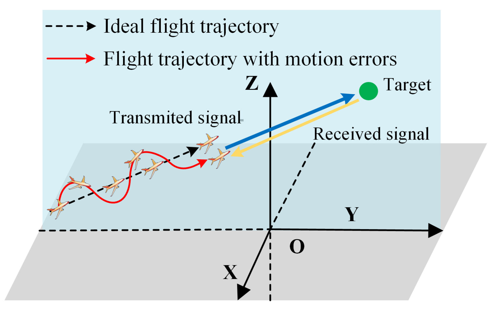
2. Signal Model
3. Principle of KT-SRAF-LVD
3.1. Principle of KT
3.2. Principle of Sinusoidal Error Compensation
3.3. Principle of LVD
3.4. Detailed Procedure of the Proposed Method
- Step 1: Perform the FFT on the pulse-compressed signal with respect to , yielding ;
- Step 2: Apply the KT to to correct the RM caused by unambiguous velocity, yielding ;
- Step 3: Perform a fold factor search on to correct the RM caused by undersampling, yielding ;
- Step 4: Apply IFFT on with respect to , yielding ;
- Step 5: Detect the target’s range cell to extract the corresponding slow time dimension signal ;
- Step 6: Apply the SRAF operation to to obtain . Then, search for the sinusoidal parameters and ;
- Step 7: Construct the phase compensation function to correct the DFM caused by sinusoidal error for , yielding . At this stage, is transformed into ;
- Step 8: Apply the LVD operation to to estimate the target’s equivalent acceleration ;
- Step 9: Construct the phase compensation function to correct the DFM caused by acceleration for , yielding ;
- Step 10: Perform the FFT on with respect to to achieve coherent integration;
- Step 11: Apply the CFAR detector for target detection.
4. Performance Analysist
4.1. Cross Terms
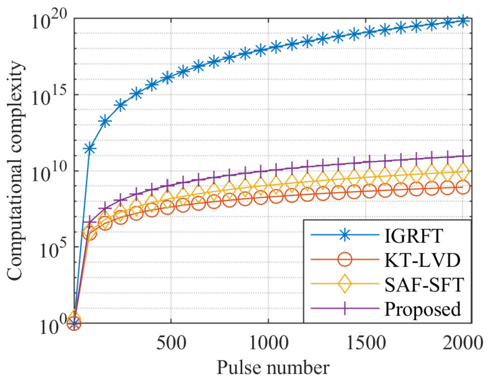
4.2. Computational Complexity
5. Simulation Results
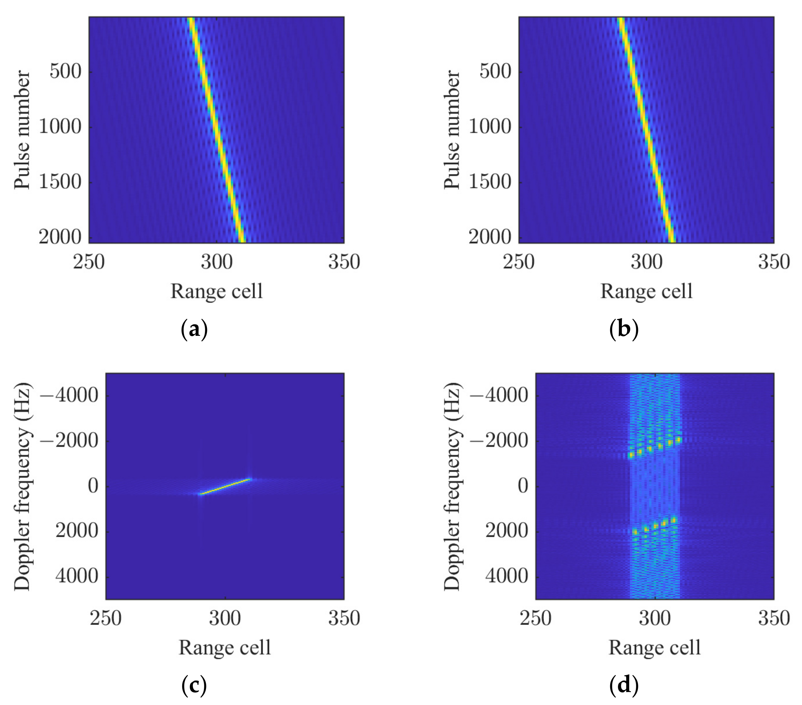
5.1. Coherent Integration for a Single Target
5.2. Coherent Integration for Multiple Targets
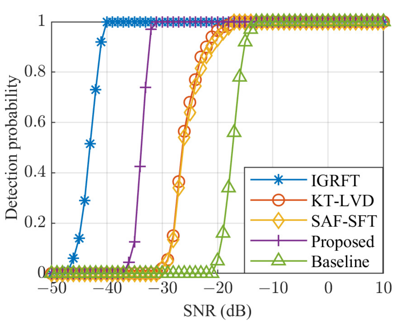
5.3. Target Detection Performance
6. Conclusions
Author Contributions
Funding
Institutional Review Board Statement
Informed Consent Statement
Data Availability Statement
Conflicts of Interest
References
- Lin, L.; Sun, G.; Cheng, Z.; He, Z. Long-time coherent integration for maneuvering target detection based on ITRT-MRFT. IEEE Sens. J. 2020, 20, 3718–3731. [Google Scholar] [CrossRef]
- He, Y.; Zhao, G.; Xiong, K. Long-Term Coherent Integration Algorithm for High-Speed Target Detection. Sensors 2024, 24, 2603. [Google Scholar] [CrossRef] [PubMed]
- Chen, X.; Guan, J.; Wang, G.; Ding, H.; Huang, Y. Fast and refined processing of radar maneuvering target based on hierarchical detection via sparse fractional representation. IEEE Access 2019, 7, 149878–149889. [Google Scholar] [CrossRef]
- Jin, K.; Li, G.; Lai, T.; Jin, T.; Zhao, Y. A novel long-time coherent integration algorithm for Doppler-ambiguous radar maneuvering target detection. IEEE Sens. J. 2020, 20, 9394–9407. [Google Scholar] [CrossRef]
- Chen, G.; Biao, X.; Jin, Y.; Xu, C.; Ping, Y.; Wang, S. Long-Time Coherent Integration Method for Passive Bistatic Radar Using Frequency Hopping Signals. Sensors 2024, 24, 6236. [Google Scholar] [CrossRef]
- Wu, Z.; Zhang, G.; Wang, X.; Sun, P.; Lin, Y. An Improved Detecting Algorithm of Moving Targets for Airborne Maritime Surveillance Radar. Sensors 2025, 25, 560. [Google Scholar] [CrossRef]
- Xu, Z.; Zhou, G. Long-time coherent integration for radar detection of maneuvering targets based on accurate range evolution model. IET Radar Sonar Navig. 2023, 17, 1558–1580. [Google Scholar] [CrossRef]
- Zhang, J.; Ding, T.; Zhang, L. Long-Time Coherent Integration Algorithm for High-Speed Maneuvering Target Detection Using Space-Based Bistatic Radar. IEEE Trans. Geosci. Remote Sens. 2022, 60, 5100216. [Google Scholar] [CrossRef]
- Yang, M.; Zhu, D.; Song, W. Comparison of two-step and one-step motion compensation algorithms for airborne synthetic aperture radar. Electron. Lett. 2015, 51, 1108–1110. [Google Scholar] [CrossRef]
- Chen, J.; Xing, M.; Yu, H.; Liang, B.; Peng, J.; Sun, G.C. Motion compensation/autofocus in airborne synthetic aperture radar: A review. IEEE Geosci. Remote Sens. Mag. 2022, 10, 185–206. [Google Scholar] [CrossRef]
- Zhang, S.S.; Zeng, T.; Long, T.; Yuan, H.-P. Dim Target Detection Based on Keystone Transform. In Proceedings of the IEEE International Radar Conference, Arlington, VA, USA, 9–12 May 2005. [Google Scholar] [CrossRef]
- Xu, J.; Yu, J.; Peng, Y.N.; Xia, X.-G. Radon-Fourier transform for radar target detection, I: Generalized Doppler filter bank. IEEE Trans. Aerosp. Electron. Syst. 2011, 47, 1186–1202. [Google Scholar] [CrossRef]
- Zheng, J.; Su, T.; Zhu, W.; He, X.; Liu, Q.H. Radar high-speed target detection based on the scaled inverse Fourier transform. IEEE J. Sel. Top. Appl. Earth Observ. Remote Sens. 2015, 8, 1108–1119. [Google Scholar] [CrossRef]
- Li, X.; Cui, G.; Yi, W.; Kong, L. Sequence-reversing transform-based coherent integration for high-speed target detection. IEEE Trans. Aerosp. Electron. Syst. 2017, 53, 1573–1580. [Google Scholar] [CrossRef]
- Xu, J.; Xia, X.G.; Peng, S.B.; Yu, J.; Peng, Y.-N.; Qian, L.-C. Radar maneuvering target motion estimation based on generalized Radon-Fourier transform. IEEE Trans. Signal Process. 2012, 60, 6190–6201. [Google Scholar] [CrossRef]
- O’Shea, P. A new technique for instantaneous frequency rate estimation. IEEE Signal Process. Lett. 2002, 9, 251–252. [Google Scholar] [CrossRef]
- O’Shea, P. A fast algorithm for estimating the parameters of a quadratic FM signal. IEEE Trans. Signal Process. 2004, 52, 385–393. [Google Scholar] [CrossRef]
- Zheng, J.; Liu, H.; Liu, Q.H. Parameterized centroid frequency-chirp rate distribution for LFM signal analysis and mechanisms of constant delay introduction. IEEE Trans. Signal Process. 2017, 65, 6435–6447. [Google Scholar] [CrossRef]
- Huang, P.; Liao, G.; Yang, Z.; Xia, X.G.; Ma, J.T.; Zhang, X. A fast SAR imaging method for ground moving target using a second-order WVD transform. IEEE Trans. Geosci. Remote Sens. 2016, 54, 1940–1956. [Google Scholar] [CrossRef]
- Lv, X.; Bi, G.; Wan, C.; Xing, M. Lv’s distribution: Principle, implementation, properties, and performance. IEEE Trans. Signal Process. 2011, 59, 3576–3591. [Google Scholar] [CrossRef]
- Li, X.; Sun, Z.; Yi, W.; Cui, G.; Kong, L.; Yang, X. Computationally efficient coherent detection and parameter estimation algorithm for maneuvering target. Signal Process. 2019, 155, 130–142.9. [Google Scholar] [CrossRef]
- Zheng, J.; Liu, H.; Liu, J.; Du, X.; Liu, Q.H. Radar high-speed maneuvering target detection based on three-dimensional scaled transform. IEEE J. Sel. Top. Appl. Earth Observ. Remote Sens. 2018, 11, 2821–2833. [Google Scholar] [CrossRef]
- Zhao, L.; Tao, H.; Chen, W. Maneuvering target detection based on three-dimensional coherent integration. IEEE Access 2020, 8, 188321–188334. [Google Scholar] [CrossRef]
- Nies, H.; Loffeld, O.; Natroshvili, K. Analysis and focusing of bistatic airborne SAR data. IEEE Trans. Geosci. Remote Sens. 2007, 45, 3342–3349. [Google Scholar] [CrossRef]
- Pu, W.; Wu, J.; Huang, Y.; Li, W.; Sun, Z.; Yang, J.; Yang, H. Motion errors and compensation for bistatic forward-looking SAR with cubic-order processing. IEEE Trans. Geosci. Remote Sens. 2016, 54, 6940–6957. [Google Scholar] [CrossRef]
- Li, J.; Chen, J.; Wang, P.; Loffeld, O. A coarse-to-fine autofocus approach for very high-resolution airborne stripmap SAR imagery. IEEE Trans. Geosci. Remote Sens. 2018, 56, 3814–3829. [Google Scholar] [CrossRef]
- Chen, S.; Lu, F.; Wang, J.; Liu, M. An Improved Phase Gradient Autofocus Method for One-Stationary Bistatic SAR. In Proceedings of the 2016 IEEE International Conference on Signal Processing, Communications and Computing (ICSPCC), Hong Kong, China, 5–8 August 2016. [Google Scholar] [CrossRef]
- Pu, W.; Wu, J.; Huang, Y.; Yang, J.; Yang, H. Fast factorized backprojection imaging algorithm integrated with motion trajectory estimation for bistatic forward-looking SAR. IEEE J. Sel. Top. Appl. Earth Observ. Remote Sens. 2019, 12, 3949–3965. [Google Scholar] [CrossRef]
- Yang, F.; Li, X.; Wang, M.; Sun, Z.; Cui, G. IGRFT-Based Signal Coherent Integration Method for High-Speed Target with Airborne Bistatic Radar. In Proceedings of the 2022 16th IEEE International Conference on Signal Processing (ICSP), Beijing, China, 21–24 October 2022. [Google Scholar] [CrossRef]
- Li, X.; Cui, G.; Yi, W.; Kong, L. Manoeuvring target detection based on keystone transform and Lv’s distribution. IET Radar Sonar Navig. 2016, 10, 1234–1242. [Google Scholar] [CrossRef]
- Pu, W.; Wu, J.; Huang, Y.; Yang, J.; Yang, H. A rise-dimensional modeling and estimation method for flight trajectory error in bistatic forward-looking SAR. IEEE J. Sel. Top. Appl. Earth Observ. Remote Sens. 2017, 10, 5001–5015. [Google Scholar] [CrossRef]
- Wang, Y.; Wang, Z.; Zhao, B.; Xu, L. Compensation for high-frequency vibration of platform in SAR imaging based on adaptive chirplet decomposition. IEEE Geosci. Remote Sens. Lett. 2016, 13, 792–795. [Google Scholar] [CrossRef]


| Parameter | Value |
|---|---|
| Carrier frequency | 10 GHz |
| Pulse repetition frequency | 10 KHz |
| Pulse width | 20 µs |
| Bandwidth | 10 MHz |
| Sampling rate | 20 MHz |
| Pulse number | 2048 |
| Parameter | Value |
|---|---|
| Initial range cell | 300 |
| Velocity | 750 m/s |
| Acceleration | 50 m/s2 |
| Parameter | Value |
|---|---|
| Amplitude | 0.8 |
| Frequency | 25 Hz |
| Method | Computational Complexity |
|---|---|
| Proposed | |
| KT-LVD | |
| SAF-SFT | |
| IGRFT |
| Parameter | Target A | Target B | Target C |
|---|---|---|---|
| Initial range cell | 300 | 300 | 300 |
| Velocity | 750 m/s | 750 m/s | 740 m/s |
| Acceleration | 20 m/s2 | 50 m/s2 | 50 m/s2 |
Disclaimer/Publisher’s Note: The statements, opinions and data contained in all publications are solely those of the individual author(s) and contributor(s) and not of MDPI and/or the editor(s). MDPI and/or the editor(s) disclaim responsibility for any injury to people or property resulting from any ideas, methods, instructions or products referred to in the content. |
© 2025 by the authors. Licensee MDPI, Basel, Switzerland. This article is an open access article distributed under the terms and conditions of the Creative Commons Attribution (CC BY) license (https://creativecommons.org/licenses/by/4.0/).
Share and Cite
Xu, W.; Wang, Y.; Cao, J.; Wang, H. KT-SRAF-LVD-Based Signal Coherent Integration Method for High-Speed Target Detecting in Airborne Radar. Sensors 2025, 25, 2128. https://doi.org/10.3390/s25072128
Xu W, Wang Y, Cao J, Wang H. KT-SRAF-LVD-Based Signal Coherent Integration Method for High-Speed Target Detecting in Airborne Radar. Sensors. 2025; 25(7):2128. https://doi.org/10.3390/s25072128
Chicago/Turabian StyleXu, Wenwen, Yuhang Wang, Jianyin Cao, and Hao Wang. 2025. "KT-SRAF-LVD-Based Signal Coherent Integration Method for High-Speed Target Detecting in Airborne Radar" Sensors 25, no. 7: 2128. https://doi.org/10.3390/s25072128
APA StyleXu, W., Wang, Y., Cao, J., & Wang, H. (2025). KT-SRAF-LVD-Based Signal Coherent Integration Method for High-Speed Target Detecting in Airborne Radar. Sensors, 25(7), 2128. https://doi.org/10.3390/s25072128