
Minimizing Redundancy in Wireless Sensor Networks Using Sparse Vectors

Abstract
1. Introduction
- At the sensor level, this paper presents an improved data-compression method. This method combines segmented regions with quartile screening to precisely locate the corresponding key values and then performs sparse vector compression. By deeply exploring the similarity between each segment of data and its corresponding key value, the amount of transmitted data can be significantly reduced.
- At the CH level, this paper optimizes the reverse sampling rate adjustment method. By fully leveraging the spatial correlation among the data of different sensor nodes, a sensor sleep decision is set. This decision can dynamically adjust the sampling frequency of active sensors within the cluster in the next cycle according to the actual network situation, effectively balancing the accuracy of data collection and energy consumption and providing a more efficient solution for energy-saving management at the CH level.
2. Methods
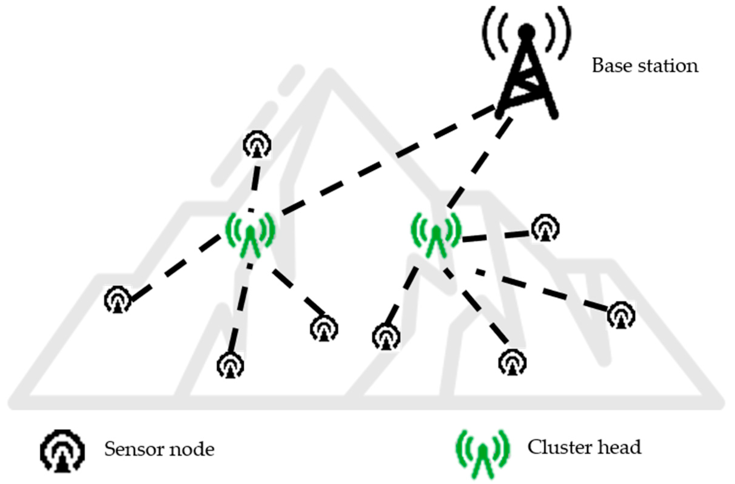
2.1. Network Model Overview
2.2. Minimizing Data Redundancy Algorithm Based on Segmented Sparse Vectors (SV-ZIZO Algorithm)
2.2.1. Indexed Bit Coding Compression Algorithm
2.2.2. Compression Method Based on Segmented Sparse Vector Representation
| Algorithm 1: Data-Split function pseudocode |
| 01 Read vector Si_p, int V 02 Set vector si_p_v 03 len_v = floor(length(Si_p)/V) 04 for v = 0 to V 05 for i = 1 to len_v len_v + i) ~= NaN len_v + i) 08 Return si_p_v |
| Algorithm 2: Key-value calculation and compression based on quartiles |
| 01 Read vector si_p_v, int ε 02 Set vector U 03 Q = [prctile(si_p_v, 25), prctile(si_p_v, 50), prctile(si_p_v, 75)] 04 m = mean(si_p_v) 05 index = min(abs(Q[1]-m), abs(Q[2]-m), abs(Q[3]-m))[2] 06 u_p_v = Q[index] 07 len_p_v = length(si_p_v) 08 Set code = zeros(len_p_v) 09 for i = 1 to len_p_v 10 if abs(si_p_v[i] − u_p_v) < ε 11 code[i] = 1 12 si_p_v[i] = NaN 13 else 14 code[i] = 0 15 c = HexToDec(code) 16 u(1) = (u_p_v, c) 17 append(U, u(1)) 18 while Si_p is all NaN 19 Set code = zeros(len_p_v) 20 u = min(si_p_v) 21 for k = 1 to len_p_v 22 if | u_i − Si_p(k)| <= ε 23 code(k) = 1 24 si_p_v[i] = NaN 25 else 26 code(k) = 0; 27 c = HexToDec(code) 28 u = (u_i, c) 29 append(U, u) 30 Return U |
2.2.3. Sensor Sampling Rate Adjustment Method at the CH Level
2.2.4. Complexity Analysis
3. Results
3.1. Parameter Settings and Evaluation Indicators
- The calculation formula of the evaluation metric Compressed Ratio (CR) is as follows:
- Calculate the average error between the reconstructed data of the i-th sensor within one cycle and the original collected data of the corresponding sensor. The calculation formula is as follows:
3.2. IBRL Dataset and Result Analysis
3.2.1. Comparison Results of Compression Ratios at the Sensor Level
3.2.2. Comparison Results of Reconstruction Accuracy at the CH Level
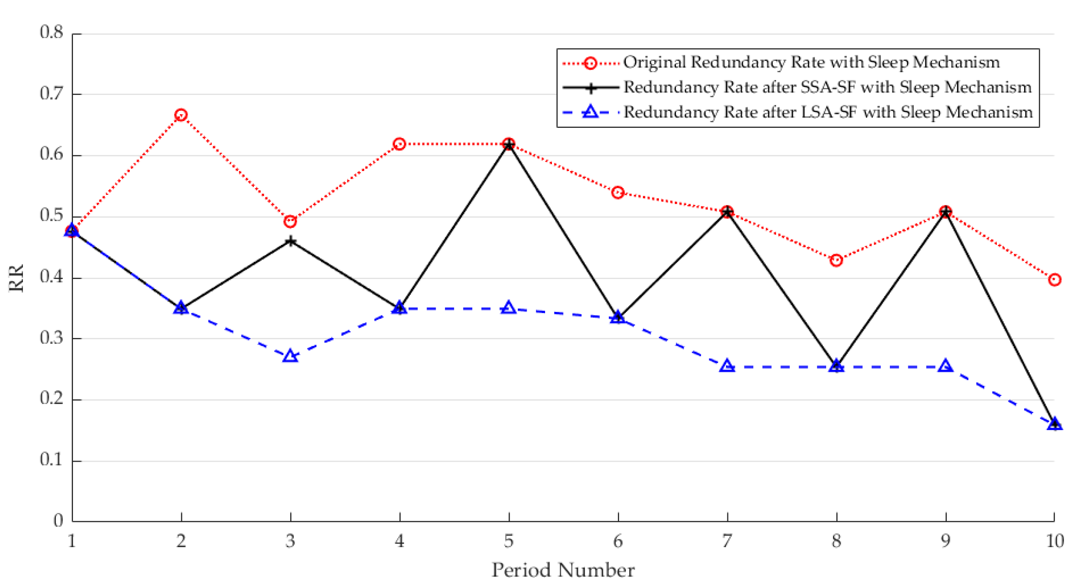
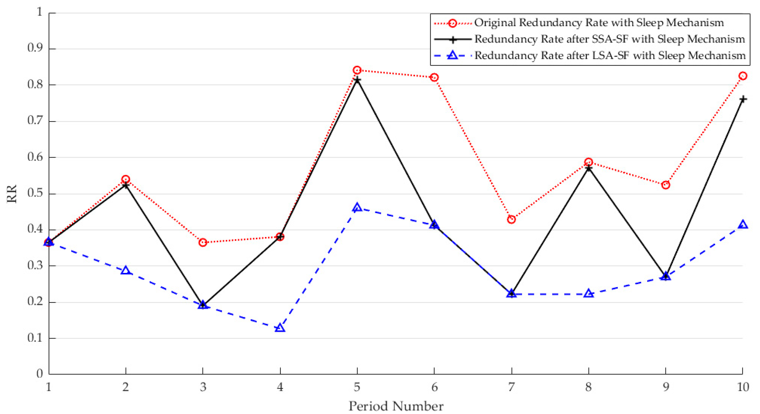
3.2.3. Adjustment Results of Dormant Sampling at the CH Level
3.2.4. Comparison Results of Total Network Energy Consumption
3.3. LUCE Dataset and Result Analysis
3.3.1. Comparison Results of Compression Ratios at the Sensor Level
3.3.2. Comparison Results of Reconstruction Accuracy at the CH Level
3.3.3. Adjustment Results of Dormant Sampling at the CH Level
3.3.4. Comparison Results of Total Network Energy Consumption
4. Conclusions
Author Contributions
Funding
Institutional Review Board Statement
Informed Consent Statement
Data Availability Statement
Conflicts of Interest
References
- Buratti, C.; Conti, A.; Dardari, D.; Verdone, R. An Overview on Wireless Sensor Networks Technology and Evolution. Sensors 2009, 9, 6869–6896. [Google Scholar] [CrossRef] [PubMed]
- Sethi, D.; Anand, J.; Tripathi, S.A. A DMA-WSN Based Routing Strategy to Maximize Efficiency and Reliability in a Ship to Communicate Data on Coronavirus. Recent Adv. Electr. Electron. Eng. 2023, 16, 579–589. [Google Scholar] [CrossRef]
- Yokoyama, T.; Narieda, S.; Naruse, H. Optimization of Sensor Node Placement for CO2 Concentration Monitoring Based on Wireless Sensor Networks in an Indoor Environment. IEEE Sens. Lett. 2024, 8, 7001904. [Google Scholar] [CrossRef]
- Rapin, M.; Braun, F.; Adler, A.; Wacker, J.; Frerichs, I.; Vogt, B.; Chetelat, O. Wearable sensors for frequency-multiplexed EIT and multilead ECG data acquisition. IEEE Trans. Biomed. Eng. 2019, 66, 810–820. [Google Scholar] [CrossRef] [PubMed]
- Qie, Y.; Hao, C.; Song, P. Wireless Transmission Method for Large Data Based on Hierarchical Compressed Sensing and Sparse Decomposition. Sensors 2020, 20, 7146. [Google Scholar] [CrossRef] [PubMed]
- AI-Qurabat AK, M.; Abdulzahra, S.A.; Idrees, A.K. Two-level energy-efficient data reduction strategies based on SAX-LZW and hierarchical clustering for minimizing the huge data conveyed on the internet of things networks. J. Supercomput. 2022, 78, 17844–17890. [Google Scholar] [CrossRef]
- Qurabat, A.; Ali, K.M.; Jaoude, C.A. Two tier data reduction technique for reducing data transmission in iot sensors. In Proceedings of the 2019 15th International Wireless Communications and Mobile Computing Conference (IWCMC), Tangier, Morocco, 24–28 June 2019; pp. 168–173. [Google Scholar]
- Saeedi ID, I.; Kadhum, A.M. Perceptually important points-based data aggregation method for wireless sensor networks. Baghdad Sci. J. 2022, 19, 875–886. [Google Scholar] [CrossRef]
- Bahi, J.; Makhoul, A.; Medlej, M. A Two Tiers Data Aggregation Scheme for Periodic Sensor Networks. Ad Hoc Sens. Wirel. Netw. 2014, 21, 77–100. [Google Scholar]
- Harb, H.; Makhoul, A.; Couturier, R.; Medlej, M. ATP: An Aggregation and Transmission Protocol for Conserving Energyin Periodic Sensor Networks. In Proceedings of the 2015 IEEE 24th International Conference on Enabling Technologies: Infrastructure for Collaborative Enterprises, Larnaca, Cyprus, 15–17 June 2015. [Google Scholar]
- Idrees, A.K.; Al-Qurabat AK, M. Energy-Efficient Data Transmission and Aggregation Protocol in Periodic Sensor Networks Based Fog Computing. J. Netw. Syst. Manag. 2020, 29, 4. [Google Scholar] [CrossRef]
- Rida, M.; Makhoul, A.; Harb, H.; Laiymani, D.; Barharrigi, M. EK-means: A new clustering approach for datasets classification in sensor networks. Ad Hoc Netw. 2019, 84, 158–169. [Google Scholar] [CrossRef]
- Changmin, L.; Jaiyong, L. Harvesting and Energy aware Adaptive Sampling Algorithm for guaranteeing self-sustainability in Wireless Sensor Network. In Proceedings of the 2017 International Conference on Information Networking (ICOIN), Da Nang, Vietnam, 11–13 January 2017. [Google Scholar]
- Sun, Y.; Yuan, Y.; Li, X.; Xu, Q.; Guan, X. An Adaptive Sampling Algorithm for Target Tracking in Underwater Wireless Sensor Networks. IEEE Access 2018, 6, 68324–68336. [Google Scholar] [CrossRef]
- Shu, T.X.; Xia, M.; Chen, J.H.; Clarence, D.S. An Energy Efficient Adaptive Sampling Algorithm in a Sensor Network for Automated Water Quality Monitoring. Sensors 2017, 17, 2551. [Google Scholar] [CrossRef]
- Basaran, M.; Schlupkothen, S.; Ascheid, G. Adaptive Sampling Techniques for Autonomous Agents in Wireless Sensor Networks. In Proceedings of the IEEE International Symposium on Personal, Indoor and Mobile Radio Communications (PIMRC), Istanbul, Turkey, 8–11 September 2019. [Google Scholar]
- Harb, H.; Makhoul, A. Energy-Efficient Sensor Data Collection Approach for Industrial Process Monitoring. IEEE Trans. Ind. Inform. 2018, 14, 661–672. [Google Scholar] [CrossRef]
- Sayed, A.E.; Harb, H.; Ruiz, M.; Esteban, L.V. ZIZO: A Zoom-In Zoom-Out Mechanism for Minimizing Redundancy and Saving Energy in Wireless Sensor Networks. IEEE Sens. J. 2021, 21, 3452–3462. [Google Scholar] [CrossRef]
- Wang, R.Z.; Lei, J.J.; Yuan, C. An optimization strategy for managing dormant nodes in wireless sensor networks base on fuzzy clustering. J. Shandong Univ. (Nat. Sci.) 2013, 48, 17–21. [Google Scholar]
- Kim, H.-J.; Baek, J.-W.; Chung, K. Associative Knowledge Graph Using Fuzzy Clustering and Min-Max Normalization in Video Contents. IEEE Access 2021, 9, 74802–74816. [Google Scholar] [CrossRef]
- Laboratory of Intelligent Sensing and Non—destructive Testing Technology, Jiangnan University. Available online: http://db.csail.mit.edu/labdata/labdata.html (accessed on 10 October 2023).
- Heinzelman, W.B. Application-Specific Protocol Architectures for Wireless Networks. Ph.D. Thesis, Massachusetts Institute of Technology, Cambridge, MA, USA, 2000. [Google Scholar]
 are abnormal sensors).
are abnormal sensors).
are abnormal sensors).


 are abnormal sensors).
are abnormal sensors).
are abnormal sensors).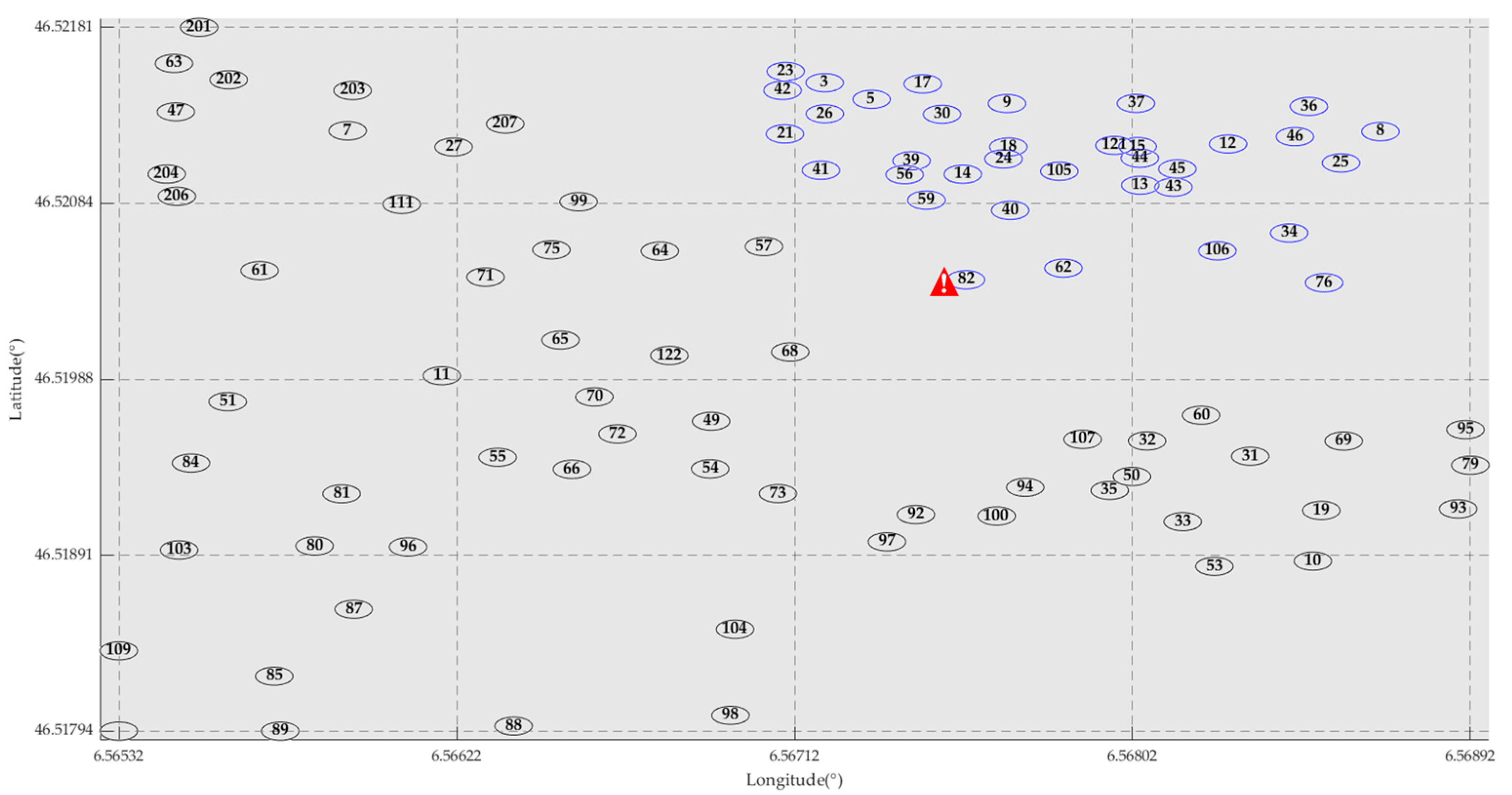


| Redundancy Rate (RR) | Large-Scale Adjustment of Sampling Frequency (LSA-SF) | Small-Scale Adjustment of Sampling Frequency (SSA-SF) |
|---|---|---|
| 0 ≤ RR ≤ 0.4 | 60% | 100% |
| 0.4 < RR ≤ 0.7 | 40% | 60% |
| 0.7 < RR ≤ 1 | 20% | 40% |
| Parameter | Values |
|---|---|
| N | IBRL: 47 LUCE: 34 |
| 32, 64 | |
| 50 nJ/bit | |
| 100 pJ/bit/m2 | |
| T | 0.2 |
| Temperature: 0.07, 0.1, 0.2 Humidity: 0.2, 0.5, 1 |
| Data Type | Period | Threshold | Algorithm 1 | SV-ZIZO(LSA-SF) | SV-ZIZO(SSA-SF) | IBE | ZIZO(LSA-SF) | ZIZO(SSA-SF) |
|---|---|---|---|---|---|---|---|---|
| Temperature | 15.53% | 10.11% | 10.70% | 12.95% | 12.59% | 12.65% | ||
| 12.10% | 7.37% | 7.63% | 10.41% | 10.13% | 10.24% | |||
| 9.97% | 6.28% | 6.55% | 6.90% | 6.87% | 6.88% | |||
| 12.29% | 9.80% | 10.99% | 9.25% | 9.01% | 9.19% | |||
| 9.09% | 5.95% | 6.56% | 7.26% | 7.09% | 7.16% | |||
| 6.33% | 4.12% | 4.36% | 4.64% | 4.59% | 4.63% | |||
| Humidity | 20.74% | 5.56% | 6.96% | 19.23% | 7.94% | 8.65% | ||
| 14.49% | 4.06% | 5.02% | 12.18% | 5.19% | 5.52% | |||
| 11.86% | 3.43% | 4.05% | 9.74% | 4.35% | 4.54% | |||
| 17.62% | 13.55% | 13.66% | 14.22% | 11.29% | 12.41% | |||
| 11.36% | 6.09% | 7.37% | 8.35% | 6.77% | 7.87% | |||
| 8.72% | 4.68% | 5.62% | 6.23% | 5.20% | 5.86% |
| Data Type | Period | Threshold | Algorithm 1 | SV-ZIZO (LSA-SF) | SV-ZIZO (SSA-SF) | IBE | ZIZO (LSA-SF) | ZIZO (SSA-SF) |
|---|---|---|---|---|---|---|---|---|
| Temperature | 11.85% | 3.48% | 3.66% | 17.16% | 6.84% | 6.86% | ||
| 8.94% | 3.03% | 3.22% | 13.35% | 5.51% | 5.62% | |||
| 6.71% | 2.62% | 2.67% | 8.78% | 3.91% | 3.94% | |||
| 8.72% | 6.55% | 7.07% | 12.96% | 11.95% | 12.46% | |||
| 5.81% | 4.52% | 4.72% | 9.69% | 9.19% | 9.44% | |||
| 3.56% | 2.85% | 2.93% | 5.99% | 5.71% | 5.81% | |||
| Humidity | 28.75% | 13.24% | 15.72% | 29.66% | 12.28% | 13.43% | ||
| 11.60% | 4.29% | 4.50% | 14.62% | 6.31% | 6.61% | |||
| 6.06% | 2.78% | 2.89% | 8.65% | 3.87% | 4.02% | |||
| 25.62% | 17.85% | 18.85% | 19.68% | 17.95% | 19.41% | |||
| 8.47% | 6.27% | 6.58% | 9.38% | 8.86% | 9.13% | |||
| 3.48% | 2.35% | 2.85% | 5.45% | 5.22% | 5.35% |
Disclaimer/Publisher’s Note: The statements, opinions and data contained in all publications are solely those of the individual author(s) and contributor(s) and not of MDPI and/or the editor(s). MDPI and/or the editor(s) disclaim responsibility for any injury to people or property resulting from any ideas, methods, instructions or products referred to in the content. |
© 2025 by the authors. Licensee MDPI, Basel, Switzerland. This article is an open access article distributed under the terms and conditions of the Creative Commons Attribution (CC BY) license (https://creativecommons.org/licenses/by/4.0/).
Share and Cite
Yuan, H.; Gao, C. Minimizing Redundancy in Wireless Sensor Networks Using Sparse Vectors. Sensors 2025, 25, 1557. https://doi.org/10.3390/s25051557
Yuan H, Gao C. Minimizing Redundancy in Wireless Sensor Networks Using Sparse Vectors. Sensors. 2025; 25(5):1557. https://doi.org/10.3390/s25051557
Chicago/Turabian StyleYuan, Huiying, and Cuifang Gao. 2025. "Minimizing Redundancy in Wireless Sensor Networks Using Sparse Vectors" Sensors 25, no. 5: 1557. https://doi.org/10.3390/s25051557
APA StyleYuan, H., & Gao, C. (2025). Minimizing Redundancy in Wireless Sensor Networks Using Sparse Vectors. Sensors, 25(5), 1557. https://doi.org/10.3390/s25051557