

Hardware Acceleration of Division-Free Quadrature-Based Square Rooting Approach for Near-Lossless Compression of Hyperspectral Images


Abstract
1. Introduction
- Introducing a division-free quadrature-based method that aims to achieve near-lossless HSI compression by reformulating the original algorithm to avoid two division operations. This method is optimized for speed and efficiency while ensuring high accuracy.
- Describing the hardware acceleration of HSI near-lossless compression while utilizing innovative seed generation and quadrature-based square rooting techniques.
- Achieving high-performance metrics targeting the Cyclone V FPGA. Synthesis results achieve a high throughput of 1611.77 Mega Samples per second (MSps) with a low power requirement of 0.886 Watts, yielding a notable efficiency value compared to existing state-of-the-art techniques.
2. Related Work
3. Near-Lossless Compression of HSI
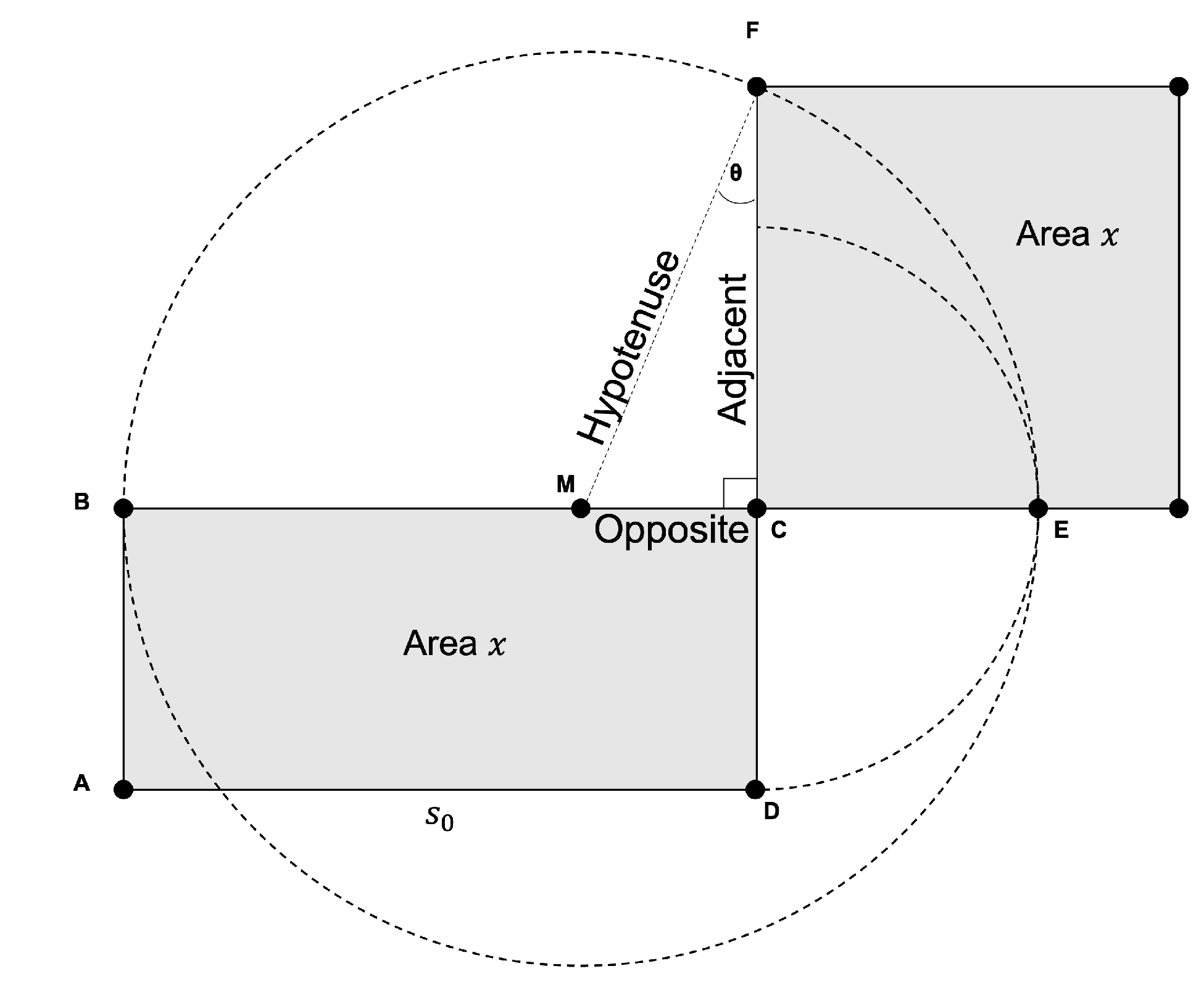
Quadrature-Based Method
| Algorithm 1: The quadrature-based square rooting method. |
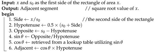 |
4. Division-Free Quadrature
4.1. Addressing the First Division
4.2. Addressing the Second Division
4.3. Performance of Quadrature-Based Method
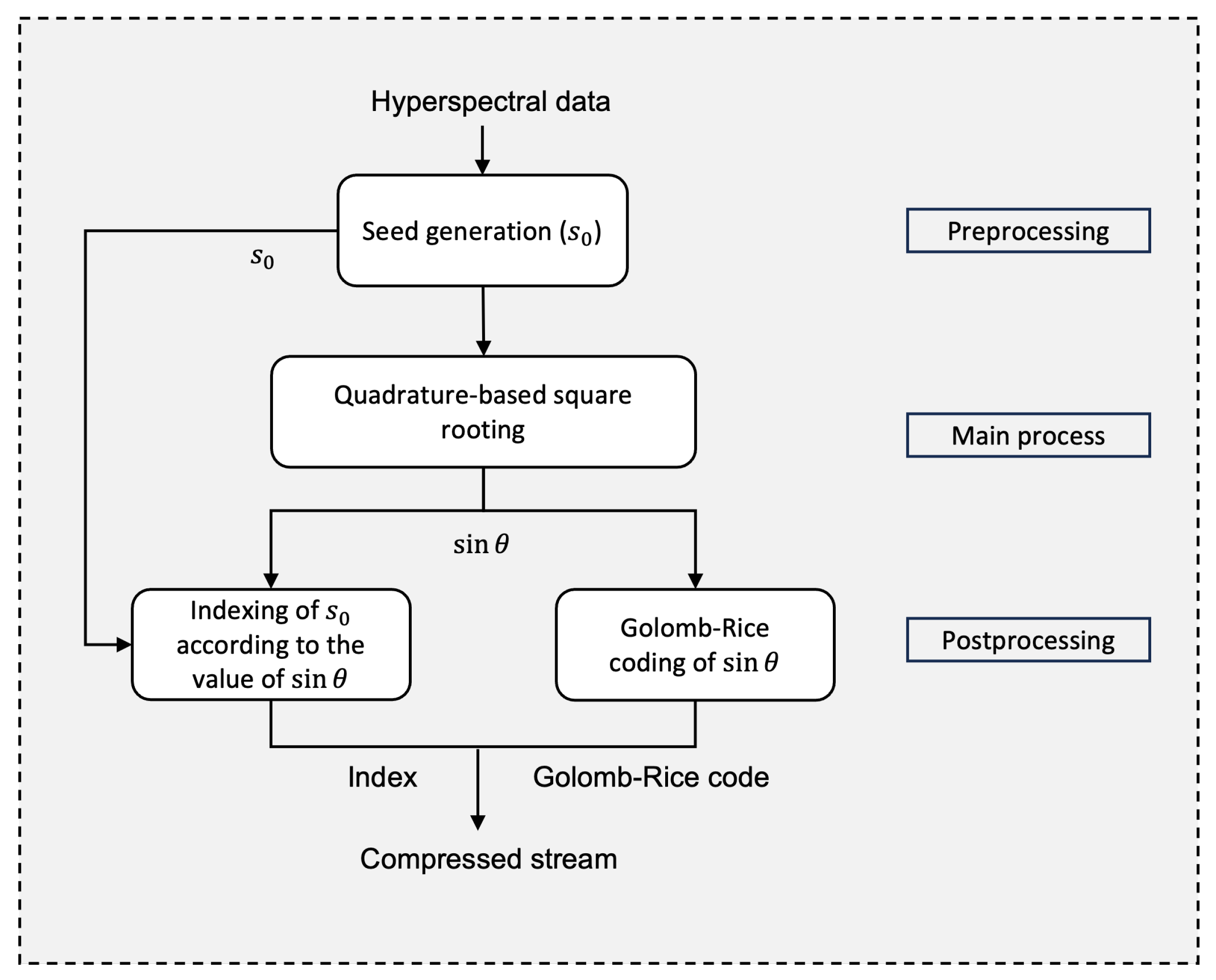
5. Hardware Implementation
5.1. Preprocessing
5.1.1. Shift-Amount Calculator
| Algorithm 2: Binary search algorithm for determining the shift amount for a 16-bit number x. |
 |
5.1.2. Seed Generation Logic
5.2. Main Process
5.2.1. First Stage of the Pipeline
5.2.2. Second Stage of the Pipeline
5.2.3. Third Stage of the Pipeline
5.2.4. Fourth Stage of the Pipeline
5.2.5. Fifth to Ninth Stages of the Pipeline
5.3. Postprocessing
5.3.1. Golomb–Rice Coding
5.3.2. Seed Indexing Logic
6. Results and Discussions
6.1. Resource Utilization and Scalability
6.2. Clock Frequency
6.3. Throughput
6.4. Power Requirement
6.5. Comparison with Division-Based Approach
6.6. Comparison with State-of-the-Art Implementations
7. Conclusions
Author Contributions
Funding
Institutional Review Board Statement
Informed Consent Statement
Data Availability Statement
Conflicts of Interest
References
- Pandey, P.C.; Balzter, H.; Srivastava, P.K.; Petropoulos, G.P.; Bhattacharya, B. Future perspectives and challenges in hyperspectral remote sensing. Hyperspectr. Remote Sens. 2020, 10, 429–439. [Google Scholar]
- Gu, Y.; Liu, T.; Gao, G.; Ren, G.; Ma, Y.; Chanussot, J.; Jia, X. Multimodal Hyperspectral Remote Sensing: An Overview and Perspective. Sci. China Inf. Sci. 2021, 64, 121301. [Google Scholar] [CrossRef]
- Mangotra, H.; Srivastava, S.; Jaiswal, G.; Rani, R.; Sharma, A. Hyperspectral imaging for early diagnosis of diseases: A review. Expert Syst. 2023, 40, e13311. [Google Scholar] [CrossRef]
- Karim, S.; Qadir, A.; Farooq, U.; Shakir, M.; Laghari, A.A. Hyperspectral imaging: A review and trends towards medical imaging. Curr. Med. Imaging 2023, 19, 417–427. [Google Scholar] [CrossRef] [PubMed]
- Yoon, J. Hyperspectral Imaging for Clinical Applications. BioChip J. 2022, 16, 1–12. [Google Scholar] [CrossRef]
- Lu, B.; Dao, P.D.; Liu, J.; He, Y.; Shang, J. Recent advances of hyperspectral imaging technology and applications in agriculture. Remote Sens. 2020, 12, 2659. [Google Scholar] [CrossRef]
- Yu, H.; Kong, B.; Hou, Y.; Xu, X.; Chen, T.; Liu, X. A critical review on applications of hyperspectral remote sensing in crop monitoring. Exp. Agric. 2022, 58, e26. [Google Scholar] [CrossRef]
- Hajaj, S.; El Harti, A.; Pour, A.B.; Jellouli, A.; Adiri, Z.; Hashim, M. A Review on Hyperspectral Imagery Application for Lithological Mapping and Mineral Prospecting: Machine Learning Techniques and Future Prospects. Remote Sens. Appl. Soc. Environ. 2024, 35, 101218. [Google Scholar] [CrossRef]
- Peyghambari, S.; Zhang, Y. Hyperspectral remote sensing in lithological mapping, mineral exploration, and environmental geology: An updated review. J. Appl. Remote Sens. 2021, 15, 031501. [Google Scholar] [CrossRef]
- Yang, H.; Kong, J.; Hu, H.; Du, Y.; Gao, M.; Chen, F. A Review of Remote Sensing for Water Quality Retrieval: Progress and Challenges. Remote Sens. 2022, 14, 1770. [Google Scholar] [CrossRef]
- Bresciani, M.; Giardino, C.; Fabbretto, A.; Pellegrino, A.; Mangano, S.; Free, G.; Pinardi, M. Application of New Hyperspectral Sensors in the Remote Sensing of Aquatic Ecosystem Health: Exploiting PRISMA and DESIS for Four Italian Lakes. Resources 2022, 11, 8. [Google Scholar] [CrossRef]
- Nisha, A.; Anitha, A. Current Advances in Hyperspectral Remote Sensing in Urban Planning. In Proceedings of the 2022 Third International Conference on Intelligent Computing Instrumentation and Control Technologies (ICICICT), Kannur, India, 11–12 August 2022; pp. 94–98. [Google Scholar]
- Li, B.; Zhang, L.; Shang, Z.; Dong, Q. Implementation of LZMA Compression Algorithm on FPGA. Electron. Lett. 2014, 50, 1522–1524. [Google Scholar] [CrossRef]
- Hasan, K.K.; Ngah, U.K.; Salleh, M.F.M. Efficient Hardware-Based Image Compression Schemes for Wireless Sensor Networks: A Survey. Wirel. Pers. Commun. 2014, 77, 1415–1436. [Google Scholar] [CrossRef]
- Benini, L.; Bruni, D.; Macii, A.; Macii, E. Memory Energy Minimization by Data Compression: Algorithms, Architectures and Implementation. IEEE Trans. Very Large Scale Integr. (VLSI) Syst. 2004, 12, 255–268. [Google Scholar] [CrossRef]
- Leavline, E.J.; Singh, D.A.A.G. Hardware Implementation of LZMA Data Compression Algorithm. Int. J. Appl. Inf. Syst. (IJAIS) 2013, 5, 51–56. [Google Scholar]
- Altamimi, A.; Ben Youssef, B. A systematic review of hardware-accelerated compression of remotely sensed hyperspectral images. Sensors 2021, 22, 263. [Google Scholar] [CrossRef] [PubMed]
- Báscones, D.; González, C.; Mozos, D. An FPGA Accelerator for Real-Time Lossy Compression of Hyperspectral Images. Remote Sens. 2020, 12, 2563. [Google Scholar] [CrossRef]
- Barrios, Y.; Rodríguez, A.; Sánchez, A.; Pérez, A.; López, S.; Otero, A.; de la Torre, E.; Sarmiento, R. Lossy Hyperspectral Image Compression on a Reconfigurable and Fault-Tolerant FPGA-Based Adaptive Computing Platform. Electronics 2020, 9, 1576. [Google Scholar] [CrossRef]
- Nascimento, J.M.P.; Véstias, M.P.; Martín, G. Hyperspectral Compressive Sensing with a System-on-Chip FPGA. IEEE J. Sel. Top. Appl. Earth Obs. Remote Sens. 2020, 13, 3701–3710. [Google Scholar] [CrossRef]
- Caba, J.; Díaz, M.; Barba, J.; Guerra, R.; de la Torre, J.A.; López, S. FPGA-based on-board hyperspectral imaging compression: Benchmarking performance and energy efficiency against GPU implementations. Remote Sens. 2020, 12, 3741. [Google Scholar] [CrossRef]
- Schwartz, C.; Sander, I.; Bruhn, F.; Persson, M.; Ekblad, J.; Fuglesang, C. Satellite image compression guided by regions of interest. Sensors 2023, 23, 730. [Google Scholar] [CrossRef] [PubMed]
- Zheng, T.; Dai, Y.; Xue, C.; Zhou, L. Recursive least squares for near-lossless hyperspectral data compression. Appl. Sci. 2022, 12, 7172. [Google Scholar] [CrossRef]
- Ansari, R.; Memon, N.D.; Ceran, E. Near-lossless image compression techniques. J. Electron. Imaging 1998, 7, 486–494. [Google Scholar]
- Beerten, J.; Blanes, I.; Serra-Sagristà, J. A fully embedded two-stage coder for hyperspectral near-lossless compression. IEEE Geosci. Remote Sens. Lett. 2015, 12, 1775–1779. [Google Scholar] [CrossRef]
- Miguel, A.; Liu, J.; Barney, D.; Ladner, R.; Riskin, E. Near-lossless compression of hyperspectral images. In Proceedings of the 2006 International Conference on Image Processing, Atlanta, GA, USA, 8–11 October 2006; pp. 1153–1156. [Google Scholar]
- Aiazzi, B.; Alparone, L.; Baronti, S. Near-lossless compression of 3-D optical data. IEEE Trans. Geosci. Remote Sens. 2001, 39, 2547–2557. [Google Scholar] [CrossRef]
- Qian, S.-E.; Bergeron, M.; Cunningham, I.; Gagnon, L.; Hollinger, A. Near lossless data compression onboard a hyperspectral satellite. IEEE Trans. Aerosp. Electron. Syst. 2006, 42, 851–866. [Google Scholar] [CrossRef]
- Wu, X.; Memon, N.; Sayood, K. A context-based, adaptive, lossless/nearly-lossless coding scheme for continuous-tone images. ISO/IEC JTC 1/SC 29/WG 1995, 1, 1–33. [Google Scholar]
- Wu, X.; Memon, N. Context-based lossless interband compression-extending CALIC. IEEE Trans. Image Process. 2000, 9, 994–1001. [Google Scholar]
- Magli, E.; Olmo, G.; Quacchio, E. Optimized onboard lossless and near-lossless compression of hyperspectral data using CALIC. IEEE Geosci. Remote Sens. Lett. 2004, 1, 21–25. [Google Scholar] [CrossRef]
- Blanes, I.; Magli, E.; Serra-Sagristà, J. A tutorial on image compression for optical space imaging systems. IEEE Geosci. Remote Sens. Mag. 2014, 2, 8–26. [Google Scholar] [CrossRef]
- Bartrina-Rapesta, J.; Blanes, I.; Aulí-Llinàs, F.; Serra-Sagristà, J.; Sanchez, V.; Marcellin, M.W. A lightweight contextual arithmetic coder for on-board remote sensing data compression. IEEE Trans. Geosci. Remote Sens. 2017, 55, 4825–4835. [Google Scholar] [CrossRef]
- Carvajal, G.; Penna, B.; Magli, E. Unified lossy and near-lossless hyperspectral image compression based on JPEG 2000. IEEE Geosci. Remote Sens. Lett. 2008, 5, 593–597. [Google Scholar] [CrossRef]
- Barrios, Y.; Sánchez, A.; Guerra, R.; Sarmiento, R. Hardware implementation of the CCSDS 123.0-B-2 near-lossless compression standard following an HLS design methodology. Remote Sens. 2021, 13, 4388. [Google Scholar] [CrossRef]
- Sánchez, A.; Blanes, I.; Barrios, Y.; Hernández-Cabronero, M.; Bartrina-Rapesta, J.; Serra-Sagristà, J.; Sarmiento, R. Reducing Data Dependencies in the Feedback Loop of the CCSDS 123.0-B-2 Predictor. IEEE Geosci. Remote Sens. Lett. 2022, 19, 6014505. [Google Scholar] [CrossRef]
- Paschalis, A.; Chatziantoniou, P.; Theodoropoulos, D.; Tsigkanos, A.; Kranitis, N. High-Performance Hardware Accelerators for Next Generation On-Board Data Processing. In Proceedings of the 2022 IFIP/IEEE 30th International Conference on Very Large Scale Integration (VLSI-SoC), Patras, Greece, 3–5 October 2022; pp. 1–4. [Google Scholar]
- Chatziantoniou, P.; Tsigkanos, A.; Theodoropoulos, D.; Kranitis, N.; Paschalis, A. An Efficient Architecture and High-Throughput Implementation of CCSDS-123.0-B-2 Hybrid Entropy Coder Targeting Space-Grade SRAM FPGA Technology. IEEE Trans. Aerosp. Electron. Syst. 2022, 58, 5470–5482. [Google Scholar] [CrossRef]
- Báscones, D.; Gonzalez, C.; Mozos, D. A real-time FPGA implementation of the CCSDS 123.0-B-2 standard. IEEE Trans. Geosci. Remote Sens. 2022, 60, 5525113. [Google Scholar] [CrossRef]
- Altamimi, A.; Ben Youssef, B. Lossless and Near-Lossless Compression Algorithms for Remotely Sensed Hyperspectral Images. Entropy 2024, 26, 316. [Google Scholar] [CrossRef] [PubMed]
- AMD. Square Root. Available online: https://docs.amd.com/r/en-US/am004-versal-dsp-engine/Square-Root (accessed on 26 June 2024).
- Consultative Committee for Space Data Systems (CCSDS). Corpus Datasets. Available online: https://cwe.ccsds.org/sls/docs/SLS-DC/123.0-B-Info/TestData/ (accessed on 4 July 2023).
- Altamimi, A.; Ben Youssef, B. Leveraging Seed Generation for Efficient Hardware Acceleration of Lossless Compression of Remotely Sensed Hyperspectral Images. Electronics 2024, 13, 2164. [Google Scholar] [CrossRef]
- Altamimi, A.; Ben Youssef, B. Novel seed generation and quadrature-based square rooting algorithms. Sci. Rep. 2022, 12, 20540. [Google Scholar] [CrossRef] [PubMed]
- Bhaskaran, V.; Konstantinides, K. Image and Video Compression Standards: Algorithms and Architectures; Kluwer Academic Publishers: Zurich, Switzerland, 2012. [Google Scholar]
- Young, C.Y. Precalculus; Wiley: London, UK, 2009; p. 966. [Google Scholar]
- Warren, H.S. Hacker’s Delight; Pearson Education: London, UK, 2013. [Google Scholar]
- Mehlhorn, K.; Sanders, P. Algorithms and data structures. Basic Toolbox 2007, 295, 160–164. [Google Scholar]
- Sedgewick, R.; Wayne, K. Algorithms; Addison-Wesley: Boston, MA, USA, 2011. [Google Scholar]


| Imager | Scene | Lossless [40] | Near-Lossless | MRE | PSNR (dB) |
|---|---|---|---|---|---|
| AVIRIS | YS *_sc00_uncal | 22% | 38.60% | 0.0102 | 50.95 |
| AVIRIS | YS_sc03_uncal | 24% | 38.60% | 0.0101 | 51.08 |
| AIRS | gran9 | 25% | 38.50% | 0.0100 | 50.61 |
| AIRS | gran16 | 26% | 38.60% | 0.0100 | 50.57 |
| AIRS | gran60 | 20% | 38.50% | 0.0100 | 50.74 |
| AIRS | gran82 | 32% | 38.60% | 0.0100 | 50.48 |
| AIRS | gran120 | 27% | 38.50% | 0.0100 | 50.61 |
| AIRS | gran126 | 22% | 38.50% | 0.0100 | 50.68 |
| AIRS | gran129 | 34% | 38.60% | 0.0100 | 50.65 |
| AIRS | gran151 | 26% | 38.50% | 0.0101 | 50.66 |
| AIRS | gran182 | 22% | 38.50% | 0.0101 | 50.71 |
| CASI | t0180f07 | 18% | 38.50% | 0.0100 | 50.23 |
| CASI | t0477f06 | 27% | 38.80% | 0.0100 | 50.28 |
| CRISM | sc182 | 37% | 38.60% | 0.0100 | 50.69 |
| Number of Bits (n) | Pivot | Shift Amount () |
|---|---|---|
| 16 | 65535 | 8 |
| 15 | 32767 | 7 |
| 14 | 16383 | 7 |
| 13 | 8191 | 6 |
| 12 | 4095 | 6 |
| 11 | 2047 | 5 |
| 10 | 1023 | 5 |
| 9 | 511 | 4 |
| 8 | 255 | 4 |
| 7 | 127 | 3 |
| 6 | 63 | 3 |
| 5 | 31 | 2 |
| 4 | 15 | 2 |
| 3 | 7 | 1 |
| 2 | 3 | 1 |
| 1 | 1 | 0 |
| Metric | Division-Based Approach | Division-Free Approach | Relative Enhancement (%) |
|---|---|---|---|
| Clock rate (MHz) | 20.77 | 84.83 * | 308.43 |
| Throughput (MSps) | 394.6 | 1611.77 | 308.46 |
| Power (Watts) | 0.783 | 0.886 | −13.15 ** |
| Efficiency (MSps/Watts) | 504 | 1819.15 | 260.94 |
| FPGA Platform | Compression Method | Throughput (MSps) | Power (Watt) | Efficiency (MSps/Watt) | Instances | Reference |
|---|---|---|---|---|---|---|
| Xilinx Kintex UltraScale | CCSDS 123.0-B-2 | 12.5 | 2.48 | 5 | NA | [35] |
| NA | CCSDS 123.0-B-2 | 125 | - | - | NA | [36] |
| Xilinx Kintex Ultrascale XCKU040 | CCSDS 123.0-B-2 | 1375 | 4.221 | 325.8 | 5 | [37] |
| Xilinx Kintex Ultrascale XCKU040 SRAM | CCSDS 123.0-B-2 | 305 | 1.525 | 200 | NA | [38] |
| Virtex-7 VC709 with XCKU040 | CCSDS 123.0-B-2 | 249.6 | 1.2 | 208 | NA | [39] |
| Cyclone V FPGA 5CGTFD9E5F35C7 | Quadrature Based | 1611.77 * | 0.886 | 1819.15 | 19 | This work |
Disclaimer/Publisher’s Note: The statements, opinions and data contained in all publications are solely those of the individual author(s) and contributor(s) and not of MDPI and/or the editor(s). MDPI and/or the editor(s) disclaim responsibility for any injury to people or property resulting from any ideas, methods, instructions or products referred to in the content. |
© 2025 by the authors. Licensee MDPI, Basel, Switzerland. This article is an open access article distributed under the terms and conditions of the Creative Commons Attribution (CC BY) license (https://creativecommons.org/licenses/by/4.0/).
Share and Cite
Altamimi, A.; Ben Youssef, B. Hardware Acceleration of Division-Free Quadrature-Based Square Rooting Approach for Near-Lossless Compression of Hyperspectral Images. Sensors 2025, 25, 1092. https://doi.org/10.3390/s25041092
Altamimi A, Ben Youssef B. Hardware Acceleration of Division-Free Quadrature-Based Square Rooting Approach for Near-Lossless Compression of Hyperspectral Images. Sensors. 2025; 25(4):1092. https://doi.org/10.3390/s25041092
Chicago/Turabian StyleAltamimi, Amal, and Belgacem Ben Youssef. 2025. "Hardware Acceleration of Division-Free Quadrature-Based Square Rooting Approach for Near-Lossless Compression of Hyperspectral Images" Sensors 25, no. 4: 1092. https://doi.org/10.3390/s25041092
APA StyleAltamimi, A., & Ben Youssef, B. (2025). Hardware Acceleration of Division-Free Quadrature-Based Square Rooting Approach for Near-Lossless Compression of Hyperspectral Images. Sensors, 25(4), 1092. https://doi.org/10.3390/s25041092