Article

A Progressive Feature Learning Network for Cordyceps sinensis Image Recognition

1
School of Computer Science, Nanjing University of Posts and Telecommunications, Nanjing 210023, China
2
Newlixon TechGroup.Co., Ltd., Nanjing 210012, China
3
School of Internet of Things, Nanjing University of Posts and Telecommunications, Nanjing 210023, China
4
State Key Laboratory of Ocean Sensing, Ocean College, Zhejiang University, Zhoushan 316021, China
*
Author to whom correspondence should be addressed.
Sensors 2025, 25(22), 7082; https://doi.org/10.3390/s25227082
Submission received: 7 September 2025 / Revised: 21 October 2025 / Accepted: 11 November 2025 / Published: 20 November 2025
(This article belongs to the Section Sensing and Imaging)

Abstract

Cordyceps sinensis (C. sinensis) is a valuable herbal medicine with wide-ranging applications. However, automating C. sinensis recognition is challenging due to the high morphological similarity and limited phenotypic variation among its subspecies. In this paper, we propose a novel approach called Progressive Feature Learning Network (PFL-Net) that mines multiple biological features to recognize different subspecies. Firstly, to comprehensively capture multi-scale discriminative features of C. sinensis, we propose the Spatial-aware Semantic Refinement Module (SSRM), which constructs discriminative feature groups by utilizing relative positions to model the intrinsic feature relations. Secondly, the Multi-scale Collaborative Perception Module (MCPM) avoids isolated biological features during modeling by establishing relations between different feature groups to enhance the recognition integrity of C. sinensis. Furthermore, to prevent the model from focusing on the same discriminative regions of C. sinensis, we propose a Channel Decouple (CD) loss that decouples features along the channel dimension, enhancing the diversity of C. sinensis discriminative features. In addition, we construct a C. sinensis dataset (CSD) to facilitate the application of biometric recognition, representing the first study focused on fine-grained C. sinensis recognition. Extensive experiments conducted on the CSD and three benchmark datasets validate the effectiveness of our proposed method, achieving a top-1 accuracy of 94.43% on the CSD dataset, which surpasses all existing approaches.

1. Introduction

Cordyceps sinensis (C. sinensis) is a rare and expensive medicinal herb, abundant in bioactive substances such as nucleotides, amino acids, polysaccharides, flavonoids, and sterols. Cordycepin, the primary constituent of authentic C. sinensis, is an alkaloid with antioxidant properties and exhibits pharmacological effects, including immune enhancement, antifatigue, and antitumor activities [1,2,3]. In Figure 1a, we present authentic and counterfeit C. sinensis samples and six core discriminative regions. Recognition of authentic C. sinensis from counterfeits poses a significant challenge, resulting in a proliferation of counterfeit products that pose a potential risk to public health. Existing recognition methods fall into two main categories. The first relies on expert experience, while the second employs multi-spectral and chemical analyses, which are both time-consuming and costly. With the advancement of computer vision [4,5,6], automatic image classification provides a new way to recognize C. sinensis accurately. To the best of our knowledge, this is the first study on image-based recognition of C. sinensis, which holds great significance for biomedicine.
C. sinensis possesses six primary discriminative features: the head, eyes, dorsal loops, front legs, middle legs, and tail legs. The recognition of C. sinensis based on expert experience requires consideration of all six biological features. Constructing multi-scale feature groups to establish discriminative regions is essential. As shown in Figure 1b, where each feature group represents a distinct discriminative region. After establishing multi-scale feature groups following expert experience, these feature groups need to be related. In Figure 1c, we establish relations between feature groups to ensure the integration of discriminative regions. This manner fully utilizes multiple regions of C. sinensis and enhances feature diversity. Different discriminative feature groups may focus on the same region, which could lead to redundancy in feature learning and hinder the ability to capture diverse and unique characteristics completely. As shown in Figure 1d, G 1 and G 1 both represent the “Eyes–Head–Dorsal loops–Front legs” features, which means they belong to the same discriminative region. Therefore, it is necessary to guide the network to focus on the six core biometric features of C. sinensis.
To address this issue, we propose a Progressive Feature Learning Network (PFL-Net), including the Spatial-aware Semantic Refinement Module (SSRM), the Multi-scale Collaborative Perception Module (MCPM), and the Channel Decouple (CD) loss. The SSRM constructs multi-scale feature groups G 1 to G n . G 1 represents the relation between local features such as “Eyes–Head–Dorsal loops–Front legs”. G n represents the relation between larger scale features such as “Eyes–Head–Dorsal loops–Front legs–Middle legs–Tail legs”. The extraction of discriminative features is enhanced by modeling the relations among the six biometric features. The MCPM is designed to establish effective relations between different feature groups. This manner prevents information loss and ensures the integrity of discriminative features. The CD operates on each feature group to further decouple features within the group, alleviating the feature coupling problem in the modeling process and guiding the network to focus on the six core biometric features of C. sinensis.
Notably, to facilitate the recognition of C. sinensis, we constructed the first C. sinensis dataset (CSD) with 17k images, significantly surpassing the scale of existing fine-grained public datasets. CSD includes 27 categories of C. sinensis, covering samples from six different regions and counterfeit. In addition, we collect images from multiple perspectives to overcome the limitations of single-angle views in capturing the C. sinensis features. In summary, the main contributions of our work are:
(1)
We propose PFL-Net, capable of accurately extracting and relating discriminative features. To the best of our knowledge, PFL-Net is the first study on recognizing C. sinensis.
(2)
The SSRM is designed to model spatial contextual, mining multi-scale discriminative features of C. sinensis. The MCPM relates the feature extracted at multiple scales to avoid the loss of C. sinensis features.
(3)
The CD loss decouples the features within the channel dimension and guides the network to focus on the C. sinensis features.
(4)
C. sinensis has significant medicinal value, we construct the first dataset for CSD. We perform extensive experiments on CSD and three fine-grained classification benchmarks demonstrating the superior performance of PFL-Net.

2. Related Work

2.1. General Image Classification

In recent years, CNN demonstrated significant potential in image classification tasks, giving rise to several representative CNN architectures, including Res2Net [7], EfficientNetV2 [8], RepVGG [9], ConvNext [10], and ConvNextV2 [11]. These models focused on classification accuracy and network scalability. Res2Net [7] improved optimization by using identity mappings for signal propagation and multi-scale convolutions to expand the receptive field. EfficientNetV2 [8] introduced a progressive learning method that improved training speed and accuracy. RepVGG [9] used reparameterization techniques to balance classification precision and performance. ConvNext [10] added independent downsampling layers to improve model stability in image classification. ConvNextV2 [11] optimized self-supervised learning for image classification by integrating neural architecture design with masked autoencoders. These methods performed well in image classification tasks but are unsuitable for fine-grained problems with large intra-class variance and small inter-class differences.

2.2. Fine-Grained Image Classification

Fine-grained image recognition aims to recognize subtle differences between objects within a supercategory, such as different subspecies of animals or cars. Existing methods are divided into three categories: bounding box annotation-based, local-based [12,13,14], and attention-based methods. First, bounding box annotation-based methods were fully supervised and required bounding box annotations in both the training and testing stages. They focused on learning discriminative mid-level features and performed well in bird species recognition and face verification. Second, local-based methods focused on learning local embeddings by predicting masked or erased regions in the image. For example, MaskCOV [12] used a covariance matrix to capture the mutual information between each quarter of randomly masked and shuffled image patches. Third, motivated by the success of attention in visual classification, TransFG [15] enhanced global discrimination by paying attention to important markers, alleviating the challenge of category variation. Notably, existing methods demonstrate strong performance on public datasets, they are suboptimal for recognizing C. sinensis, which exhibits complex biological characteristics and structurally similar variants.

3. Method

3.1. Overview Architecture

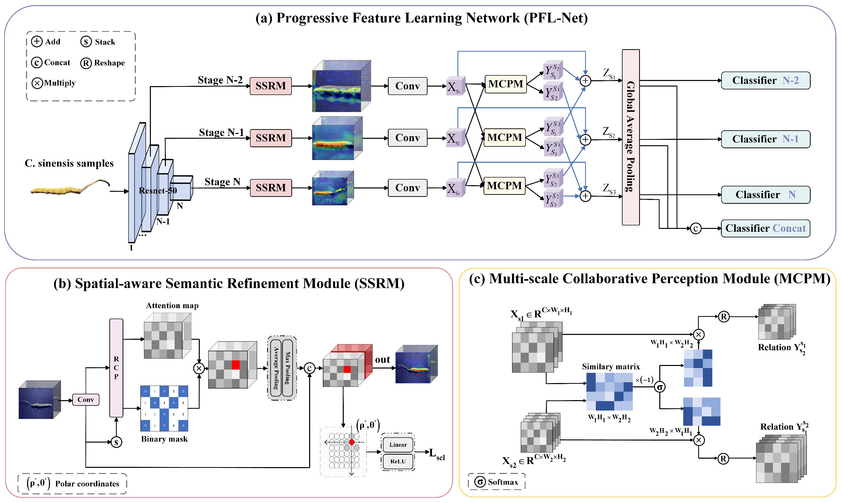
In Figure 2a, the proposed Progressive Featuer Learning Network (PFL-Net) is composed of a backbone ResNet50 [4], SSRM, and MCPM. Let F represent our backbone feature extractor, which consists of N stages. The output feature map from any intermediate stage is denoted as F n , with n = { 1 , 2 , , N } .
The SSRM applies at each intermediate stage of the backbone to extract feature maps. We use the output F n of the n-th intermediate stage of the backbone as the input of the SSRM module, denoted as V n = SSRM ( F n ) . The output vector V n of each stage then passes through MCPM, denoted as { X n , X n 1 } = MCPM ( V n ) .
The classification module f c l s n , consisting of two fully connected layers, predicts the probability distribution over classes for the n -th stage, denoted as y n = f c l s n ( X n ) . The features extracted at the shallow level cannot fully demonstrate the biological features of Cordyceps sinensis, and the mining ability is limited. Therefore, we consider the final 3 stages: n = n , n 1 , n 2 . Lastly, we concatenate the outputs from the last three stages as follows [4,16]:
y c a t = f c l s c a t ( c o n c a t [ X n 2 , X n 1 , X n ] )

3.2. Spatial-Aware Semantic Refinement Module

CNN extracts structural features through convolution and gradually integrates features across layers to form a multi-level representation. Spatial structural information is crucial for C. sinensis image recognition. As shown in Figure 2b, we propose a Spatial-aware Semantic Refinement Module (SSRM) that builds feature groups by learning the spatial context information of the object, thereby enhancing the feature representation capability of the backbone network.
For the input image I, SSRM directly applies to the feature map f ( I ) extracted by the backbone. First, convolution is performed on the feature map to obtain h ( l ) R C × N × N , which represents the spatial information of different features. The spatial relation of various features can be obtained by modeling the structural information between different parts of C. sinensis.
This paper uses polar coordinates to measure spatial relations between different regions. The traditional Cartesian coordinate system effectively measures linear distances but is sensitive to rotation and scale changes when modeling spatial relationships within an object [17]. In contrast, the polar coordinate system ( r , θ ) represents spatial layouts using radial distance and angle relative to a central point, offering inherent rotation invariance and scale adaptability. In biological image recognition, where structures such as the head, body, and tail of Cordyceps sinensis exhibit axial or radial organization, polar coordinates provide a more robust means of capturing geometric and topological relationships, ensuring stable modeling of structural coherence and spatial dependencies [18]. Given a reference region R o = R x , y , indexed at ( x , y ) on the N × N plane, and a reference horizontal direction, the polar coordinates of the region R i , j can be written as ( r i , j , θ i , j ) :
r i , j = 1 N ( x i ) 2 + ( y j ) 2 2
θ i , j = ( a t a n 2 ( y j , x i ) + π ) 2 π
where r i , j measures the relative distance. θ i , j measures the polar angle of R i , j relative to the horizontal direction. a t a n 2 ( · ) is a function that calculates the angle between two points. In this paper, we select the region with the maximum response m ( I ) as the reference region:
R o = R x , y , ( x , y ) = arg max 1 x , y N m ( I ) i , j
The SSRM utilizes polar coordinates to guide the module in learning and identifying the features of C. sinensis. Specifically, the SSRM module calculates the polar coordinates of the region R i , j by analyzing the discriminant information of the target region R i , j and the reference region R 0 . This process involves channel-wise concatenation of the feature map h ( l ) with h ( I ) x , y , followed by a fully connected layer to generate the predicted polar coordinates ( r i , j , θ i , j ) . The SSRM module models the spatial structure between different parts of an object and integrates the object region mask m ( I ) learned from the backbone network.
The SSRM first measures the relative distance differences between all regions and the object:
L d = I I 1 i , j N m ( I ) i , j ( r i , j r i , j ) 2 m ( I )
The second measures the angular difference between regions within the object. The structural information of an object should be rotationally invariant and robust to various appearances and poses. Therefore, we calculate the angle loss L a using the standard deviation of the difference between the predicted and true polar angles, as follows:
L a = I I 1 i , j N m ( I ) i , j θ Δ i , j θ ¯ Δ 2 m ( I )
θ Δ i , j = θ i , j θ i , j , if θ i , j θ i , j 0 1 + θ i , j θ i , j , otherwise ,
θ ¯ Δ = 1 m ( I ) 1 i , j N m ( I ) i , j θ Δ i , j
where θ ¯ Δ represents the average difference between the predicted polar angle and the actual polar angle. SSRM models the relative structure between object parts. During polar coordinate regression, the predicted semantic mask m ( I ) filters out irrelevant visual information outside the main object. In general, the loss function of SSRM can be expressed as:
L s s r m = L d + L a
The polar-coordinate-based losses supervise the network to learn structural consistency between predicted and ground-truth spatial relations. Specifically, the distance loss L d penalizes deviations in the relative radial distances between regions, ensuring scale consistency. The angular loss L a constrains the predicted angular relations to maintain rotational invariance and correct part ordering. Jointly minimizing L d + L a enforces the backbone to encode spatial geometry of C. sinensis parts in a biologically meaningful manner, improving robustness to pose and orientation variations. Through SSRM, the backbone learns and recognizes the structural features of the object, enabling the backbone network to model the spatial dependencies between the parts of the object and mine features.

3.3. Multi-Scale Collaborative Perception Module

Given the importance of learning discriminative and diverse features in Fine-grained Image Classification (FGIC) [18,19,20,21], we propose the Multi-scale Collaborative Perception Module (MCPM). The module enhances the expressiveness of local features by aggregating complementary information from different scales, improving feature discriminability and diversity.
Figure 2c briefly illustrates the structure of the MCPM. To demonstrate the Effectiveness of the approach, we denote two different scale feature representations as X s 1 R C × W 1 H 1 and X s 2 R C × W 2 H 2 . The subscript s i indicates that X s i focuses on the ith part of the object. We regard the feature vector at each spatial location in the channel dimension as a pixel, as follows:
p x ( X , i ) = ( X 1 , i , , X C , i ) T
where p x stands for pixels. We first compute the similarity between the pixels in X s 1 and those in X s 2 :
M = f ( X p 1 , X p 2 ) , f ( X , Y ) = X T Y
We use the inner product to compute the similarity. The M i , j represents the similarity between the ith pixel of X s 1 and the ith pixel of X s 2 . The lower the similarity between two pixels, the greater their complementarity. Therefore, we use M as the complementarity matrix. We then normalize M along both the row and column directions, as follows:
A s 1 s 2 = œ ( M T ) [ 0 , 1 ] A s 2 s 1 = œ ( M ) [ 0 , 1 ]
where œ is softmax, the operation is applied column-wise. This allows us to obtain the complementary information:
Y s 1 s 2 = X s 2 A s 1 s 2 R C × W 1 H 1 Y s 2 s 1 = X s 1 A s 2 s 1 R C × W 2 H 2
where Y s j s i represents the complementary information of X s i with respect to X s j . Each pixel of Y s 2 s 1 can be written as:
p x ( Y s 1 s 2 , i ) = j [ 1 , W 2 H 2 ] ( A s 1 s 2 ) i , j × p x ( X p 2 , j )
Each pixel in Y s 1 s 2 uses all pixels of X s 2 as a reference. The higher the complementarity between p x ( X s 1 , i ) and p x ( X s 2 , j ) , the greater the contribution of p x ( X s 2 , j ) to p x ( Y s 1 s 2 , i ) . Thus, each pixel within these scale features can capture semantically complementary information from other pixels. In the normal case, given a set of part-specific features S = { X s 1 , X s 2 , X s 3 , , X s n } , the complementary information of X s i is:
Y s i = X s j P i j Y s i s j
The Y s 1 s 2 can be obtained by applying X s i and X s j to Equations (13), (14) and (16). We can compute both Y s i s j and Y s j s i simultaneously. This results in the enhanced object features:
Z s i = X s i + γ × Y s i
where γ is a hyperparameter controlling the diversification degree, default set to 2.

3.4. Loss Function

During feature learning, excessive focus on the same discriminative regions can occur. To address this, we propose a Channel Decouple (CD) loss, which decouples features and mitigates feature coupling. After inputting an image into the network, we extract the feature map, denoted as F R C × W × H , with height H, width W, and number of channels C. We need to set the value of C equal to c × k , where c and k indicate the number of classes in a dataset and the number of feature channels used to represent each class. The nth vector feature channel of F is represented as F n R W H , n = 1 , 2 , , N . Each channel matrix of F is reshaped into a vector of size W H . The grouped feature channels corresponding to the ith class are represented as F i R k × W H , i = 0 , 1 , , c 1 . This can be expressed as:
F i = F i × k + 1 , F i × k + 2 , . . . , F i × k + k
The feature group F = { F 0 , F 1 , , F c 1 } is processed through two parallel streams in the network, each designed with a distinct sub-loss tailored for two different objectives. In the cross-entropy stream, F is treated as the input to a fully connected layer with the traditional CE [22]. The CE encourages the network to extract informative features focused primarily on global discriminative regions. On the other hand, the CD stream supervises the network to highlight different local discriminative regions. A specific number of grouped feature channels is representative of each class. The discriminative component enforces class alignment among the feature channels, ensuring that each feature channel corresponding to a specific class has sufficient discriminative power. L C D can be expressed as:
L C D ( F ) = L C E ( y , 1 i = 0 c 1 e g ( F i ) e g ( F 0 ) , , e g ( F c 1 ) T )
where g ( · ) is defined as:
g ( F i ) = 1 W H k = 1 W H max j = 1 , 2 , , ξ M i · F i , j , k
where M i is a random mask between 0 and 1. The cross-entropy (CE) and Channel Decouple (CD) losses are optimized jointly in a parallel manner. The backbone features are simultaneously fed into two loss branches: one for global discrimination (CE stream) and one for local feature diversification (CD stream). During training, the gradients from both loss functions are backpropagated to the shared feature extractor, with the total loss formulated as
L o s s ( F ) = L C E ( F ) + μ × L C D ( F )
The weighting coefficient μ controls the relative influence of the CD loss. Empirically, we set μ = 0.3 to balance global classification accuracy and feature diversity. This joint optimization ensures that the model simultaneously enhances discriminability and suppresses channel redundancy.

4. Data Collection and Construction

4.1. Material Preparation

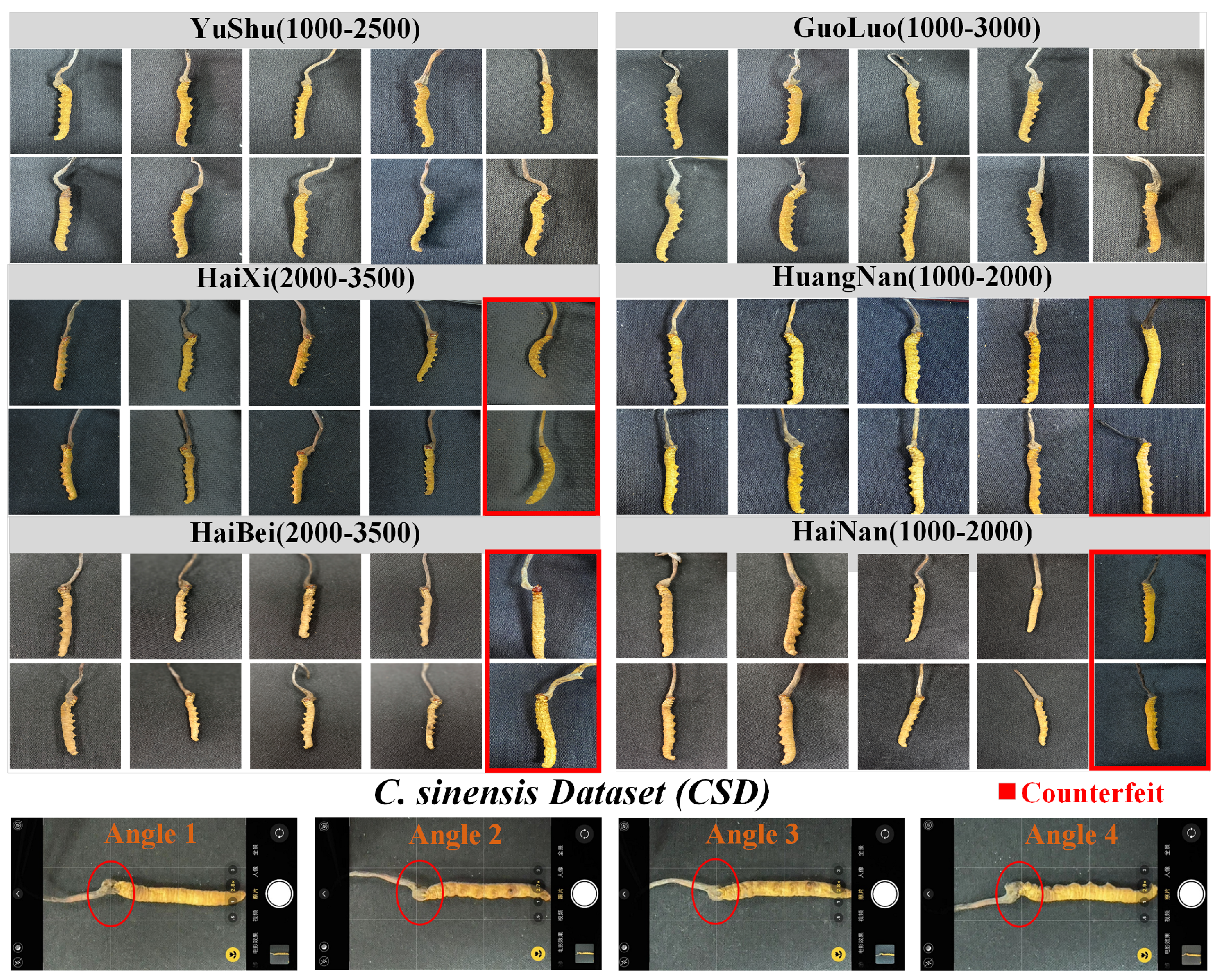
We purchased and collected 654 Cordyceps sinensis (C. sinensis) samples, covering six major production regions and including counterfeit samples. The pharmacological efficacy of C. sinensis is strongly influenced by its place of origin, with the six major production regions being Yushu, Guoluo, Haixi, Hainan, Haibei, and Huangnan. As shown in Figure 3, we present two sample images for each specification of C. sinensis from each production area. Counterfeit samples refer to artificially synthesized C. sinensis, which have no medicinal value and may harm health. Each region’s C. sinensis samples vary in size, defined by the number of specimens per 500 g. Smaller sizes correspond to larger individual specimens, which generally have higher medicinal value. We then proceeded to capture images of these samples.

4.2. Data Collection and Annotation

Images are collected using eight smart devices, including both Android and iOS devices, covering a wide range of popular devices. The images of C. sinensis were taken from four angles: the back, the foot, the left side, and the right side. As shown in Figure 3 the last row. To ensure data consistency and minimize background interference, all images were captured using the camera’s nine-grid layout, with the C. sinensis positioned within the central three grids and the eyes aligned along the first horizontal line. A ring light was placed above the specimens to optimize imaging conditions and capture fine details, while a standardized black background was used to reduce background noise. The final dataset comprises over 17k images. Table 1 presents the number of C. sinensis images collected for each specification from different production regions.
To ensure reproducibility, the CSD dataset was randomly divided into five balanced subsets using a fixed random seed (seed = 1024). Each subset preserves the class distribution across all 27 categories. During 5-fold cross-validation, four subsets were used for training and one for testing in each iteration, ensuring no overlap between training and test samples. This partitioning principle guarantees consistency across repeated experiments.

Environmental Considerations and Optical Stability

Although the dataset was collected under controlled illumination using a ring light and standardized background, the quality of captured images may still be influenced by subtle environmental factors such as air turbulence, humidity, and temperature fluctuations during shooting. These conditions can induce wavefront aberrations and minor defocus effects that alter the sharpness and spatial coherence of fine-grained texture details. Previous optical studies [23] have demonstrated that turbulent environments can distort the wavefront propagation of light, leading to random phase errors and reduced contrast in microscopic structures. While our imaging setup minimizes such disturbances, potential optical aberrations may still affect the precision of spatial feature extraction, especially for thin or reflective specimens of C. sinensis. In future work, incorporating adaptive optics or turbulence-aware image correction techniques could further improve the robustness of fine-grained feature acquisition under non-ideal environmental conditions.

5. Experiments

5.1. Datasets and Settings

Data. In the CSD, we use 70% of the images for training and the remaining 30% for testing, consistent with the public datasets. To verify the generalization ability of our proposed PFL-Net, we conducted comprehensive experiments on three public fine-grained recognition benchmarks: CUB-200-2011 (CUB) [24], Stanford Cars (CAR) [25], and FGVC-Aircraft (AIR) [26]. In Table 2, we followed the standard procedure for splitting the training and testing images and used top-1 accuracy as the evaluation metric.
Implementation Details. We used ResNet50 [4] as backbone networks. In the experiment, we only used image labels for supervised training, random cropping, horizontal flipping augmentation during training, and center cropping during testing. The input image size is 448 × 448. The SGD optimizer is used with a momentum of 0.9 and weight decay 5 × 10⁻⁴. The learning rate of the backbone layer is 0.0002, and the learning rate of the new layer is 0.002, both adjusted according to the cosine annealing strategy [27]. The learning rate of the auxiliary classifier is kept constant at 0.01. The model is trained for 200 rounds and is trained end-to-end on Nvidia RTX 3090 (Nvidia, Santa Clara, CA, USA) based on PyTorch 2.1.1.

5.2. Comparison with State of the Arts

Table 3 presents the experimental results of the comparative evaluation on the CSD, CUB-200-2011, Stanford Cars, and FGVC-Aircraft. We proposed that PFL-Net consistently outperforms state-of-the-art methods on both the CSD dataset and the three widely used benchmarks. The enhancement in performance is due to the design of our network and the efficiency of its components.
PFL-Net surpasses methods that leverage implicit data augmentation, such as DCL [38], ISDA [28], and LearnableISDA [31], demonstrating its superior ability to capture fine-grained details. In addition, PFL-Net outperforms attention-based methods like S3Ns [36], ACNet [34], AP-CNN [33], and P2P-Net [40]. While PMG [37] achieved promising results by aggregating images, PFL-Net further enhances the learning of inter-class differences by mining multi-scale features and fusing information across scales via the MCPM. PFL-Net significantly outperforms PMG [37] in classification accuracy. Compared to API-Net [35], PFL-Net achieves superior classification performance without the need to construct specific image pairs. Furthermore, PFL-Net outperforms Bi-FRN [30] and C2-Net [29] by eliminating the need to construct support-query sample pairs. It places greater emphasis on the relationships between features, resulting in generally superior classification performance.

5.3. Ablation Studies

To evaluate the effectiveness of the key components in our proposed approach, we conducted ablation experiments on CSD and CUB [24]. The results are shown in Table 4. The introduction of SSRM improves accuracy by +1.16% on CSD, demonstrating the benefit of spatial context modeling. MCPM further enhances accuracy by +1.39% through cross-scale feature collaboration. Finally, incorporating the CD loss provides an additional +1.39% gain by encouraging channel diversity and reducing redundant focus. Overall, PFL-Net achieves a total improvement of +2.79% over the baseline, validating the effectiveness of each component.
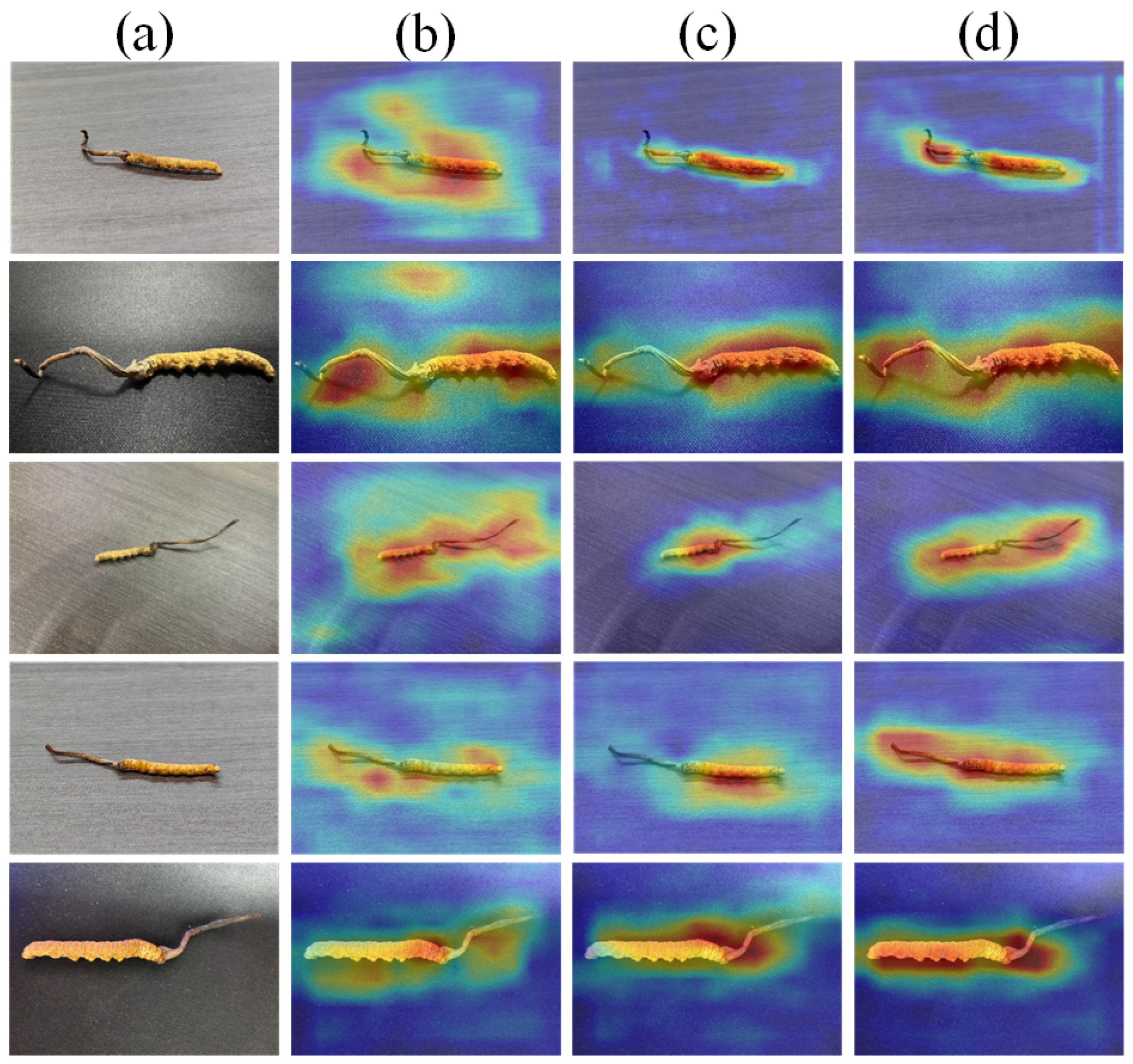
Specifically, as shown in Figure 4, SSRM provides a spatial context modeling manner, which helps to mine the discriminative features of C. sinensis. In addition, MCPM can associate the discriminative regions of C. sinensis to avoid information loss. The overall performance can be further improved owing to the complementary nature of SSRM and MCPM. Furthermore, we use CD loss to decouple features and guide the network to focus on the core discriminative features of C. sinensis. The results show that our Progressive Feature Learning Network can fully identify each feature region of C. sinensis.

5.4. Visualizations

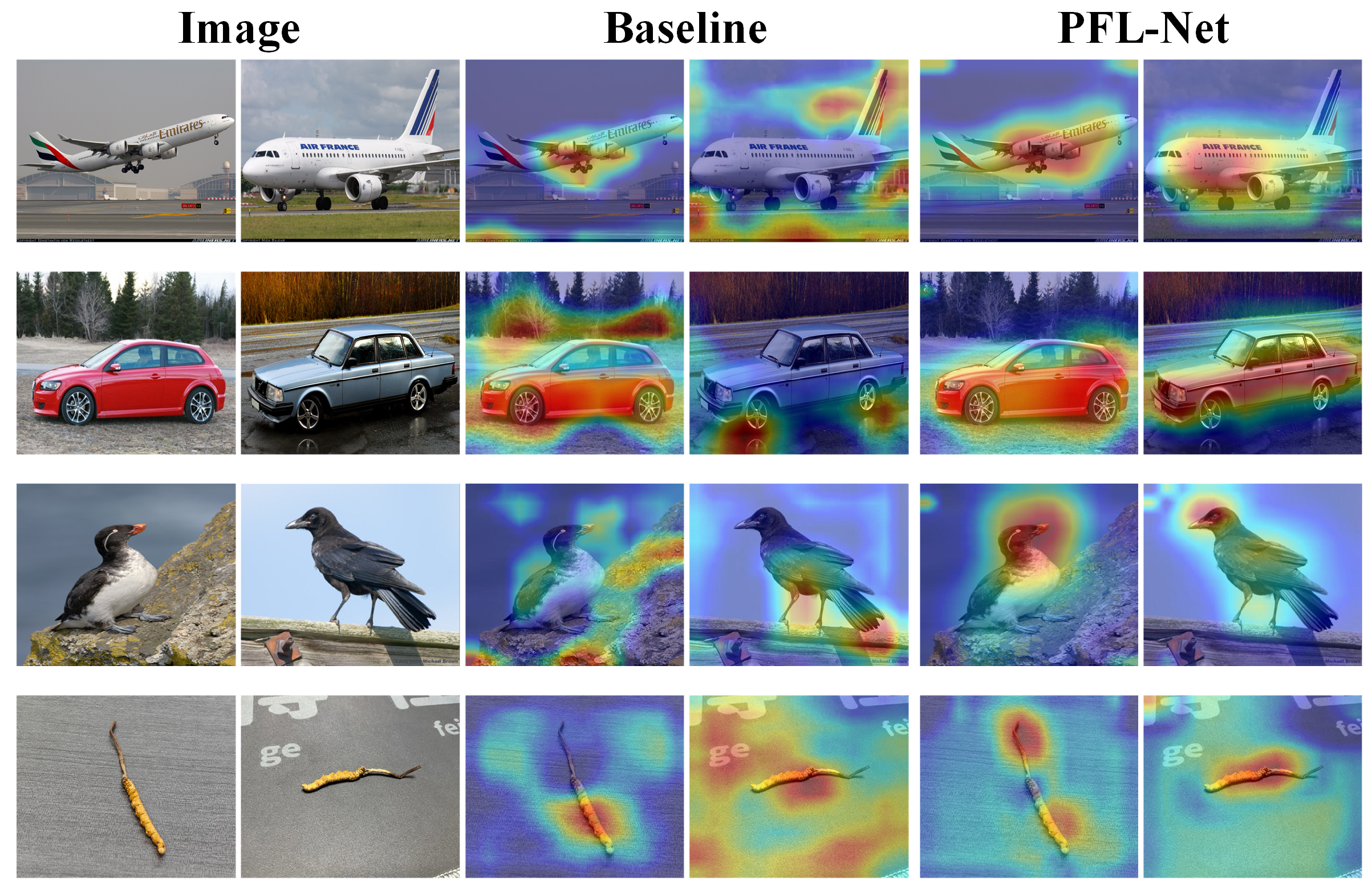
Class Activation Map—We further apply Grad-CAM [41] to the final convolutional layer to provide intuitive visualizations. Figure 5 displays the activation maps for four datasets. Compared to the baseline model, PFL-Net focuses more on discriminative regions of the target object, such as the body of an airplane, the main contours of a car, the head of a bird, and the morphological features of C. sinensis. In addition, PFL-Net exhibits significantly lower activation in background areas, demonstrating its effectiveness in suppressing noise and irrelevant information. Visualizations across multiple datasets reveal that PFL-Net effectively extracts more category-specific regions, creating clearer boundaries between the object and background.
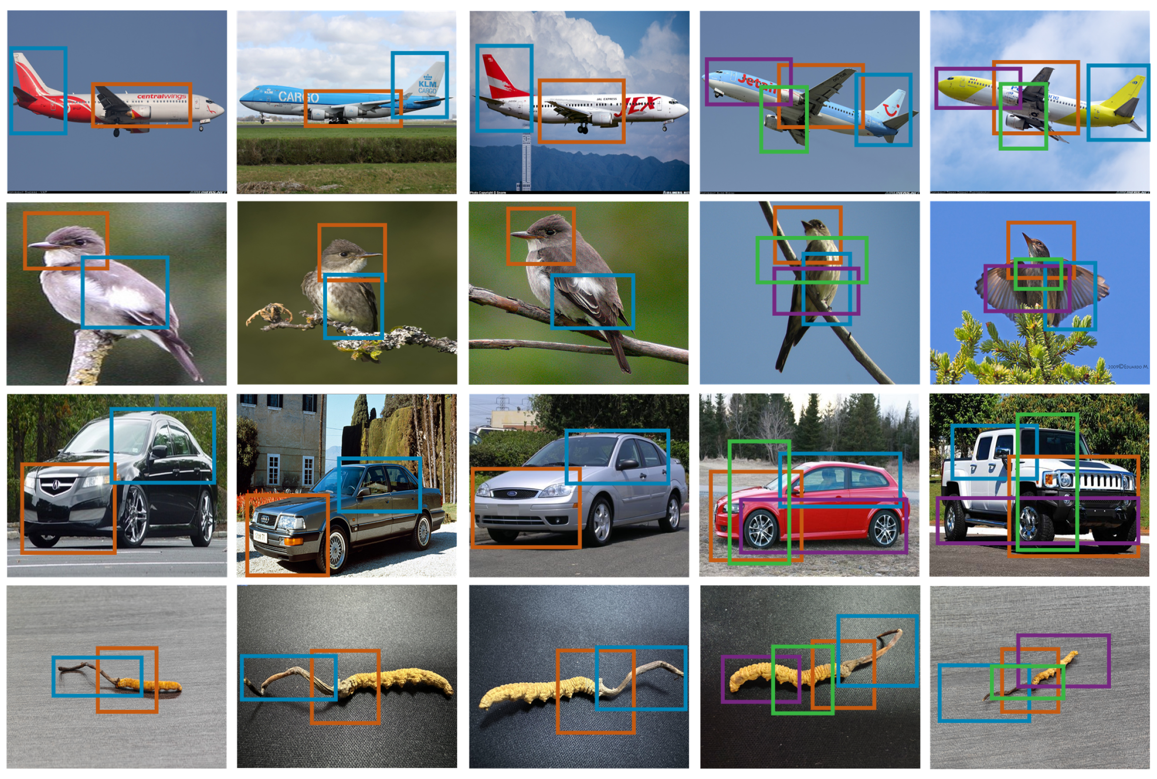
Parts Location—The discriminative regions identified by our PFL-Net are shown in Figure 6. Columns 1 to 3 display bounding boxes for only the first two parts, while columns 4 and 5 show all four primary discriminative regions. As illustrated, the first two regions exhibit notable similarities: for aircraft, they are the wings and tail; for birds, the head and body; for cars, the front and roof; for C. sinensis, they are the head and eyes. PFL-Net is capable of accurately and efficiently recognizing these key discriminative regions, demonstrating high robustness.
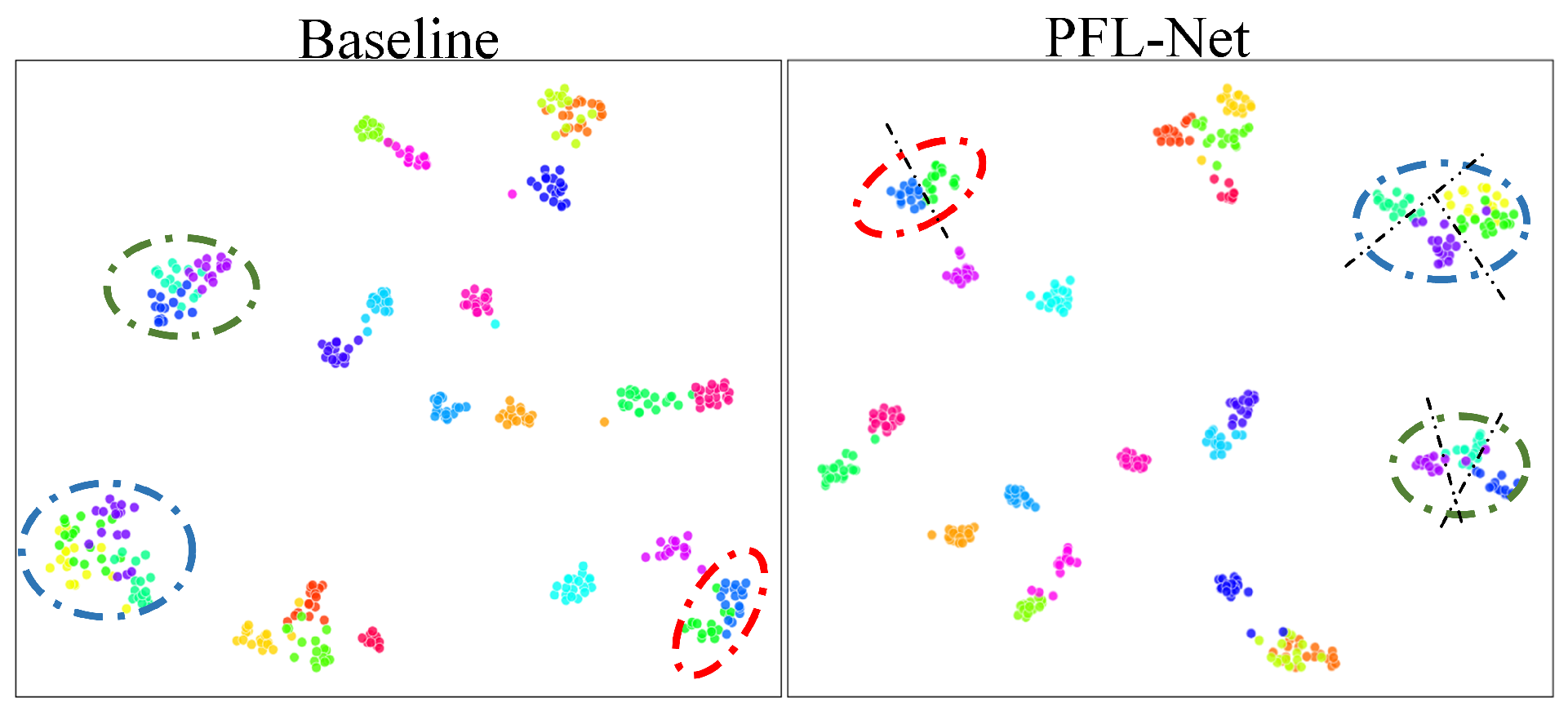
Feature Visualization—To intuitively evaluate the separability of features learned by the proposed PFL-Net, we employ the t-distributed Stochastic Neighbor Embedding (t-SNE) [42,43,44] to project high-dimensional features into a two-dimensional space for visualization, as shown in Figure 7. t-SNE is a nonlinear dimensionality reduction method that preserves the local neighborhood structure of data by modeling pairwise similarities between samples in both high-dimensional and low-dimensional spaces. Given two samples x i and x j in the high-dimensional feature space, their similarity is modeled by a conditional probability:
p j | i = exp x i x j 2 / 2 σ i 2 k i exp x i x k 2 / 2 σ i 2 ,
where σ i controls the variance of the Gaussian kernel centered at x i . In the low-dimensional embedding, the similarity between points y i and y j is defined as:
q i j = 1 + y i y j 2 1 k l 1 + y k y l 2 1 .
t-SNE minimizes the Kullback–Leibler (KL) divergence between these two distributions:
L t - SNE = i j p i j log p i j q i j ,
ensuring that nearby points in the high-dimensional space remain close in the low-dimensional visualization, while distant points are pushed apart. This results in an embedding that effectively preserves local similarities and reveals cluster structures. As illustrated in Figure 7, the features extracted by PFL-Net form more compact intra-class clusters and exhibit clearer inter-class boundaries compared to the baseline, indicating superior discriminative feature representation and robustness in fine-grained classification tasks.
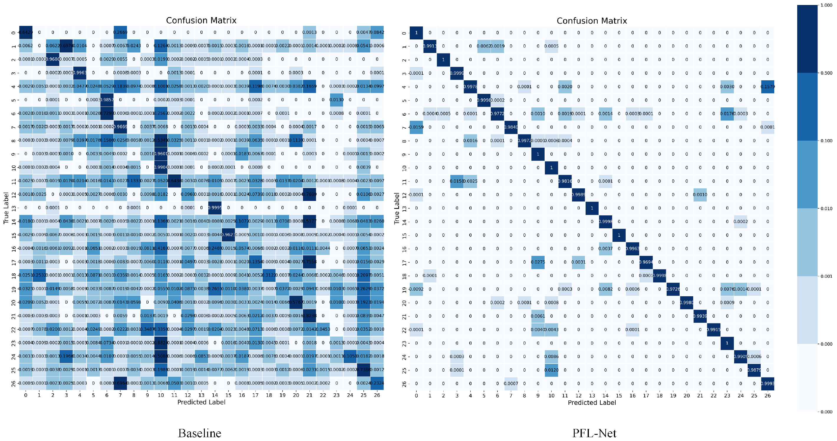
Confusion Matrix—As shown in Figure 8, the left matrix illustrates the confusion matrix of the baseline model, where the diagonal elements are scattered and many off-diagonal entries exhibit noticeable values, indicating frequent misclassifications among visually similar subspecies. This suggests that the baseline model struggles to learn discriminative representations for categories with subtle morphological differences. In contrast, the right panel presents the confusion matrix of PFL-Net, where nearly all the values are concentrated along the main diagonal, and off-diagonal elements are close to zero. This demonstrates that PFL-Net can accurately distinguish among all 27 C. sinensis categories, including those with highly similar appearances. The improved performance results from the integration of the Spatial-aware Semantic Refinement Module (SSRM) and Multi-scale Collaborative Perception Module (MCPM), which enable the model to better capture fine-grained spatial relationships and maintain feature consistency across scales. Overall, PFL-Net achieves clearer classification boundaries, lower confusion rates, and stronger generalization across subspecies.

6. Conclusions

This paper is the first to study the recognition task of Cordyceps sinensis, constructing a dedicated dataset and proposing a Progressive Feature Learning Network (PFL-Net) to promote the development of recognition in the biomedical field. By effectively combining the Spatial-aware Semantic Refinement Module (SSRM) and Multi-scale Collaborative Perception Module (MCPM), PFL-Net enhances the relation between local and global features, improving its ability to recognize complex structures. The Channel Decoupling (CD) loss further optimizes the network to extract diverse features. Experiments on Cordyceps sinensis dataset and three fine-grained classification benchmarks indicate that PFL-Net achieves state-of-the-art performance, and visualization results demonstrate its effectiveness. In the future, PFL-Net has the potential to be applied to other biological recognition scenarios.

Limitations and Future Work

Although PFL-Net achieves promising results, several limitations remain. First, the model relies on high-quality annotations and balanced category distributions; significant noise or imbalance in the dataset may affect its stability. Second, while the Spatial-aware Semantic Refinement Module (SSRM) provides spatial robustness, extreme variations in illumination or occlusion may still degrade feature consistency. Third, the multi-scale collaborative design slightly increases computational cost compared to lightweight architectures. Future work will focus on optimizing model efficiency and extending PFL-Net to other biological recognition domains with more diverse imaging conditions.

Author Contributions

Conceptualization, S.Y.; Data curation, W.W.; Formal analysis, S.L.; Funding acquisition, S.L., H.C., L.M. and Y.J.; Investigation, S.L.; Methodology, S.L.; Project administration, W.W., H.C. and F.Z.; Supervision, H.C., S.Y., L.M., F.Z. and Y.J.; Validation, L.M.; Visualization, S.L. and W.W.; Writing—original draft, W.W.; Writing—review & editing, S.Y. and J.L. All authors have read and agreed to the published version of the manuscript.

Funding

This work was supported by Jiangsu Newlixon TechGroup.Co., Ltd Project (KJ20240106), Jiangsu Key Development Planning Project (BE2023004-2).

Institutional Review Board Statement

Not applicable.

Informed Consent Statement

Not applicable.

Data Availability Statement

The data presented in this study are available on request from the corresponding author.

Acknowledgments

We would like to express our gratitude to Newlixon for their financial support and the provision of equipment used in our experiments. Their generous contributions were instrumental in the successful completion of this research.

Conflicts of Interest

Yimu Ji’s supervision, the affiliation does not provide any financial support or funding. Authors Haijun Chen and Lin Mao were employed by the company Newlixon TechGroup.Co., Ltd. The remaining authors declare that the research was conducted in the absence of any commercial or financial relationships that could be construed as a potential conflict of interest. The funding sponsors had no role in the design of the study; in the collection, analyses, or interpretation of data; in the writing of the manuscript; or in the decision to publish the results.

References

  1. Liang, J.; Li, X.; Chen, J.; Tang, C.; Wang, T.; Li, Y. Suitability and regionalization of Chinese cordyceps in Qinghai Province, Northwest China. Mycosystema 2022, 41, 1772–1785. [Google Scholar]
  2. Liu, W.; Gao, Y.; Zhou, Y.; Yu, F.; Li, X.; Zhang, N. Mechanism of cordyceps sinensis and its extracts in the treatment of diabetic kidney disease: A review. Front. Pharmacol. 2022, 13, 881835. [Google Scholar] [CrossRef] [PubMed]
  3. Krishna, K.V.; Ulhas, R.S.; Malaviya, A. Bioactive compounds from Cordyceps and their therapeutic potential. Crit. Rev. Biotechnol. 2024, 44, 753–773. [Google Scholar] [CrossRef]
  4. He, K.; Zhang, X.; Ren, S.; Sun, J. Deep residualearning for image recognition. In Proceedings of the CVPR, Las Vegas, NV, USA, 26 June–1 July 2016; pp. 770–778. [Google Scholar]
  5. Du, F.; Yang, P.; Jia, Q.; Nan, F.; Chen, X.; Yang, Y. Global and local mixture consistency cumulative learning for long-tailed visual recognitions. In Proceedings of the CVPR, Vancouver, BC, Canada, 10–22 June 2023; pp. 15814–15823. [Google Scholar]
  6. Fang, F.; Liu, Y.; Xu, Q. Localizing discriminative regions for fine-grained visual recognition: One could be better than many. Neurocomputing 2024, 610, 128611. [Google Scholar] [CrossRef]
  7. Gao, S.H.; Cheng, M.M.; Zhao, K.; Zhang, X.Y.; Yang, M.H.; Torr, P. Res2net: A new multi-scale backbone architecture. IEEE Trans. Pattern Anal. Mach. Intell. 2019, 43, 652–662. [Google Scholar] [CrossRef]
  8. Tan, M.; Le, Q. Efficientnetv2: Smaller models and faster training. In Proceedings of the ICML, Online, 18–24 July 2021; pp. 10096–10106. [Google Scholar]
  9. Ding, X.; Zhang, X.; Ma, N.; Han, J.; Ding, G.; Sun, J. Repvgg: Making vgg-style convnets great again. In Proceedings of the CVPR, Online, 19–25 June 2021; pp. 13733–13742. [Google Scholar]
  10. Liu, Z.; Mao, H.; Wu, C.Y.; Feichtenhofer, C.; Darrell, T.; Xie, S. A convnet for the 2020s. In Proceedings of the CVPR, New Orleans, LS, USA, 21–24 June 2022; pp. 11976–11986. [Google Scholar]
  11. Woo, S.; Debnath, S.; Hu, R.; Chen, X.; Liu, Z.; Kweon, I.S.; Xie, S. Convnext v2: Co-designing and scaling convnets with masked autoencoders. In Proceedings of the CVPR, Vancouver, BC, Canada, 10–22 June 2023; pp. 16133–16142. [Google Scholar]
  12. Yu, X.; Zhao, Y.; Gao, Y.; Xiong, S. Maskcov: A random mask covariance network for ultra-fine-grained visual categorization. Pattern Recognit. 2021, 119, 108067. [Google Scholar] [CrossRef]
  13. Song, J.; Yang, R. Feature boosting, suppression, and diversification for fine-grained visual classification. In Proceedings of the IJCNN, Shenzhen, China, 18–22 July 2021; pp. 1–8. [Google Scholar]
  14. Yu, X.; Zhao, Y.; Gao, Y. SPARE: Self-supervised part erasing for ultra-fine-grained visual categorization. Pattern Recognit. 2022, 128, 108691. [Google Scholar] [CrossRef]
  15. He, J.; Chen, J.N.; Liu, S.; Kortylewski, A.; Yang, C.; Bai, Y.; Wang, C. Transfg: A transformer architecture for fine-grained recognition. In Proceedings of the AAAI, Online, 22 February–1 March 2022; Volume 36, pp. 852–860. [Google Scholar]
  16. LeCun, Y.; Bengio, Y.; Hinton, G. Deep learning. Nature 2015, 521, 436–444. [Google Scholar] [CrossRef] [PubMed]
  17. Xie, E.; Wang, W.; Ding, M.; Zhang, R.; Luo, P. Polarmask++: Enhanced polar representation for single-shot instance segmentation and beyond. IEEE Trans. Pattern Anal. Mach. Intell. 2021, 44, 5385–5400. [Google Scholar] [CrossRef] [PubMed]
  18. Behera, A.; Wharton, Z.; Hewage, P.R.; Bera, A. Context-aware attentional pooling (cap) for fine-grained visual classification. In Proceedings of the AAAI, Online, 2–9 February 2021; Volume 35, pp. 929–937. [Google Scholar]
  19. Liu, C.; Xie, H.; Zha, Z.J.; Ma, L.; Yu, L.; Zhang, Y. Filtration and distillation: Enhancing region attention for fine-grained visual categorization. In Proceedings of the AAAI, New York, NY, USA, 7–12 February 2020; Volume 34, pp. 11555–11562. [Google Scholar]
  20. Zhao, Y.; Li, J.; Chen, X.; Tian, Y. Part-guided relational transformers for fine-grained visual recognition. IEEE Trans. Image Process. 2021, 30, 9470–9481. [Google Scholar] [CrossRef] [PubMed]
  21. Sun, G.; Cholakkal, H.; Khan, S.; Khan, F.; Shao, L. Fine-grained recognition: Accounting for subtle differences between similar classes. In Proceedings of the AAAI, New York, NY, USA, 7–12 February 2020; Volume 34, pp. 12047–12054. [Google Scholar]
  22. Murphy, K.P. Probabilistic Machine Learning: An Introduction; MIT Press: Cambridge, MA, USA, 2022. [Google Scholar]
  23. Khorin, P.; Dzyuba, A.; Khonina, S. Optical wavefront aberration: Detection, recognition, and compensation techniques—A comprehensive review. Opt. Laser Technol. 2025, 191, 113342. [Google Scholar] [CrossRef]
  24. Welinder, P.; Branson, S.; Mita, T.; Wah, C.; Schroff, F.; Belongie, S.; Perona, P. Caltech-UCSD Birds 200; Caltech: Pasadena, CA, USA, 2010. [Google Scholar]
  25. Dataset, E. Novel datasets for fine-grained image categorization. In Proceedings of the CVPR, Colorado Springs, CO, USA, 20–25 June 2011; Volume 5, p. 2. [Google Scholar]
  26. Maji, S.; Rahtu, E.; Kannala, J.; Blaschko, M.; Vedaldi, A. Fine-grained visual classification of aircraft. arXiv 2013, arXiv:1306.5151. [Google Scholar] [CrossRef]
  27. He, T.; Zhang, Z.; Zhang, H.; Zhang, Z.; Xie, J.; Li, M. Bag of tricks for image classification with convolutional neural networks. In Proceedings of the CVPR, Long Beach, CA, USA, 16–20 June 2019; pp. 558–567. [Google Scholar]
  28. Wang, Y.; Pan, X.; Song, S.; Zhang, H.; Huang, G.; Wu, C. Implicit semantic data augmentation for deep networks. NeurIPS 2019, 32, 12614–12623. [Google Scholar]
  29. Ma, Z.X.; Chen, Z.D.; Zhao, L.J.; Zhang, Z.C.; Luo, X.; Xu, X.S. Cross-Layer and Cross-Sample Feature Optimization Network for Few-Shot Fine-Grained Image Classification. In Proceedings of the AAAI, Vancouver, BC, USA, 20–28 February 2024; Volume 38, pp. 4136–4144. [Google Scholar]
  30. Wu, J.; Chang, D.; Sain, A.; Li, X.; Ma, Z.; Cao, J.; Guo, J.; Song, Y.Z. Bi-directional feature reconstruction network for fine-grained few-shot image classification. In Proceedings of the AAAI, Washington, DC, USA, 7–15 February 2023; Volume 37, pp. 2821–2829. [Google Scholar]
  31. Pu, Y.; Han, Y.; Wang, Y.; Feng, J.; Deng, C.; Huang, G. Fine-grained recognition with learnable semantic data augmentation. IEEE Trans. Image Process. 2024, 33, 3130–3144. [Google Scholar] [CrossRef] [PubMed]
  32. Rahman, S.; Koniusz, P.; Wang, L.; Zhou, L.; Moghadam, P.; Sun, C. Learning partial correlation based deep visual representation for image classification. In Proceedings of the CVPR, Vancouver, BC, USA, 18–22 June 2023; pp. 6231–6240. [Google Scholar]
  33. Ding, Y.; Ma, Z.; Wen, S.; Xie, J.; Chang, D.; Si, Z.; Wu, M.; Ling, H. AP-CNN: Weakly supervised attention pyramid convolutional neural network for fine-grained visual classification. IEEE Trans. Image Process. 2021, 30, 2826–2836. [Google Scholar] [CrossRef] [PubMed]
  34. Ji, R.; Wen, L.; Zhang, L.; Du, D.; Wu, Y.; Zhao, C.; Liu, X.; Huang, F. Attention convolutional binary neural tree for fine-grained visual categorization. In Proceedings of the CVPR, Seattle, WA, USA, 13–19 June 2020; pp. 10468–10477. [Google Scholar]
  35. Zhuang, P.; Wang, Y.; Qiao, Y. Learning attentive pairwise interaction for fine-grained classification. In Proceedings of the AAAI, New York, NY, USA, 7–12 February 2020; Volume 34, pp. 13130–13137. [Google Scholar]
  36. Ding, Y.; Zhou, Y.; Zhu, Y.; Ye, Q.; Jiao, J. Selective sparse sampling for fine-grained image recognition. In Proceedings of the ICCV, Seoul, Republic of Korea, 27 October–2 November 2019; pp. 6599–6608. [Google Scholar]
  37. Du, R.; Chang, D.; Bhunia, A.K.; Xie, J.; Ma, Z.; Song, Y.Z.; Guo, J. Fine-grained visual classification via progressive multi-granularity training of jigsaw patches. In Proceedings of the ECCV, Online, 23–28 August 2020; pp. 153–168. [Google Scholar]
  38. Chen, Y.; Bai, Y.; Zhang, W.; Mei, T. Destruction and construction learning for fine-grained image recognition. In Proceedings of the CVPR, Long Beach, CA, USA, 16–20 June 2019; pp. 5157–5166. [Google Scholar]
  39. Alexey, D. An image is worth 16 × 16 words: Transformers for image recognition at scale. In Proceedings of the ICLR, Virtual Event, 3–7 May 2021; p. 11929. [Google Scholar]
  40. Yang, X.; Wang, Y.; Chen, K.; Xu, Y.; Tian, Y. Fine-grained object classification via self-supervised pose alignment. In Proceedings of the CVPR, New Orleans, LS, USA, 19–23 June 2022; pp. 7399–7408. [Google Scholar]
  41. Selvaraju, R.R.; Cogswell, M.; Das, A.; Vedantam, R.; Parikh, D.; Batra, D. Grad-cam: Visual explanations from deep networks via gradient-based localization. In Proceedings of the ICCV, Nicosia, Cyprus, 24–25 April 2017; pp. 618–626. [Google Scholar]
  42. Van der Maaten, L.; Hinton, G. Visualizing data using t-SNE. J. Mach. Learn. Res. 2008, 9, 2579–2605. [Google Scholar]
  43. Wattenberg, M.; Viégas, F.; Johnson, I. How to Use t-SNE Effectively. Distill 2016, 1, e2. [Google Scholar] [CrossRef]
  44. Belkina, A.C.; Ciccolella, C.O.; Anno, R.; Spidlen, J.; Snyder-Cappione, J.E. Automated optimal parameters for t-distributed stochastic neighbor embedding improve visualization and allow analysis of large datasets. Nat. Commun. 2019, 10, 5415. [Google Scholar] [PubMed]
Figure 1. (a) illustrates authentic and counterfeit C. sinensis samples, highlighting six core discriminative features, while (bd) detail the analysis process of multi-scale features of C. sinensis.
Sensors 25 07082 g001
Figure 2. (a) The overall architecture of PFL-Net includes a feature extractor, the Spatial-aware Semantic Refinement Module(SSRM), and the Multi-scale Collaborative Perception Module(SSRM). “N” represents the number of stages in the backbone network. (b) shows the structure of the SSRM. (c) illustrates the MCPM.
Sensors 25 07082 g002
Figure 3. The C. sinensis dataset consists of Cordyceps sinensis samples from six major production regions, along with counterfeit samples. Dataset shooting rules are shown on the last line.
Sensors 25 07082 g003
Figure 4. Visualization of ablation experiments. (a) input, (b) Baseline, (c) Baseline + SSRM + MCPM, and (d) PFL-Net.
Sensors 25 07082 g004
Figure 5. Class Activation Map on four datasets.
Sensors 25 07082 g005
Figure 6. Discriminative regions detected by our PFL-Net.
Sensors 25 07082 g006
Figure 7. A t-SNE plot of learned representations on CSD.
Sensors 25 07082 g007
Figure 8. Confusion matrix on CSD.
Sensors 25 07082 g008
Table 1. Distribution of C. sinensis products by origin, specification (number of pieces per 500 g), and number of images.
OriginSpecificationImageOriginSpecificationImage
Yushu1000636Guoluo1000600
12006261200640
15006201500640
20005682000592
25006163000576
Haixi2000636Huangnan1000616
25006401200584
30006161500636
35006162000640
Haibei2000616Hainan1000640
25006401200624
30006361500600
35006402000640
Counterfeit/3167
Table 2. Overview of the public datasets used in our experiments, including the number of classes, training, and test samples for each dataset.
DatasetClassesTrainingTesting
CUB-200-2011 [24]20059945794
Stanford Cars [25]19681448041
FGVC-Aircraft [26]10066673333
Table 3. The top-1 accuracy (%) comparison with state-of-the-art methods on the CSD, CUB-200-2011, Stanford Cars, and FGVC-Aircraft datasets is presented. Bold values indicate the best results, and underlined values represent the second-best results.
MethodVenueC. sinensis DatasetCUB-200-2011Stanford CarsFGVC-Aircraft
ISDA [28]NeurIPS1981.485.391.793.2
C2-Net [29]AAAI2488.584.6-88.9
Bi-FRN [30]AAAI2389.985.4-88.4
LearnableISDA [31]TIP2490.286.792.794.3
iSICE [32]CVPR2390.285.993.592.7
AP-CNN [33]TIP2190.587.292.293.6
ACNet [34]CVPR2090.688.192.494.6
API-Net [35]AAAI2091.087.793.094.8
S3Ns [36]ICCV1991.288.592.894.7
PMG [37]ECCV2092.188.992.895.0
DCL [38]CVPR1992.887.893.094.5
ViT [39]ICLR2193.190.394.294.8
P2P-Net [40]CVPR2293.290.294.994.2
TransFG [15]AAAI2293.791.794.8-
PFL-Net (our)-94.491.294.995.1
Table 4. Ablation studies on the CSD and CUB (using original images) are conducted with the baseline (ResNet50) to evaluate the impact of different modules.
IndexComponentAccuracy (%)
BaselineSSRMMCPMCDCSDCUB
0 91.6488.88
1 92.8089.02
2 91.8789.93
3 93.0389.41
4 93.3490.95
5 94.1990.55
6 93.7590.41
794.4391.26
Disclaimer/Publisher’s Note: The statements, opinions and data contained in all publications are solely those of the individual author(s) and contributor(s) and not of MDPI and/or the editor(s). MDPI and/or the editor(s) disclaim responsibility for any injury to people or property resulting from any ideas, methods, instructions or products referred to in the content.