Author Contributions
Conceptualization, E.-K.L.; Methodology, D.J.J. and S.A.; Software, D.J.J. and S.A.; Validation, D.J.J. and S.A.; Formal analysis, E.-K.L.; Investigation, D.J.J., S.A. and E.-K.L.; Resources, E.-K.L.; Data curation, D.J.J., S.A. and E.-K.L.; Writing—original draft, D.J.J. and S.A.; Writing—review & editing, E.-K.L.; Visualization, D.J.J. and S.A.; Supervision, E.-K.L.; Project administration, E.-K.L.; Funding acquisition, E.-K.L. All authors have read and agreed to the published version of the manuscript.
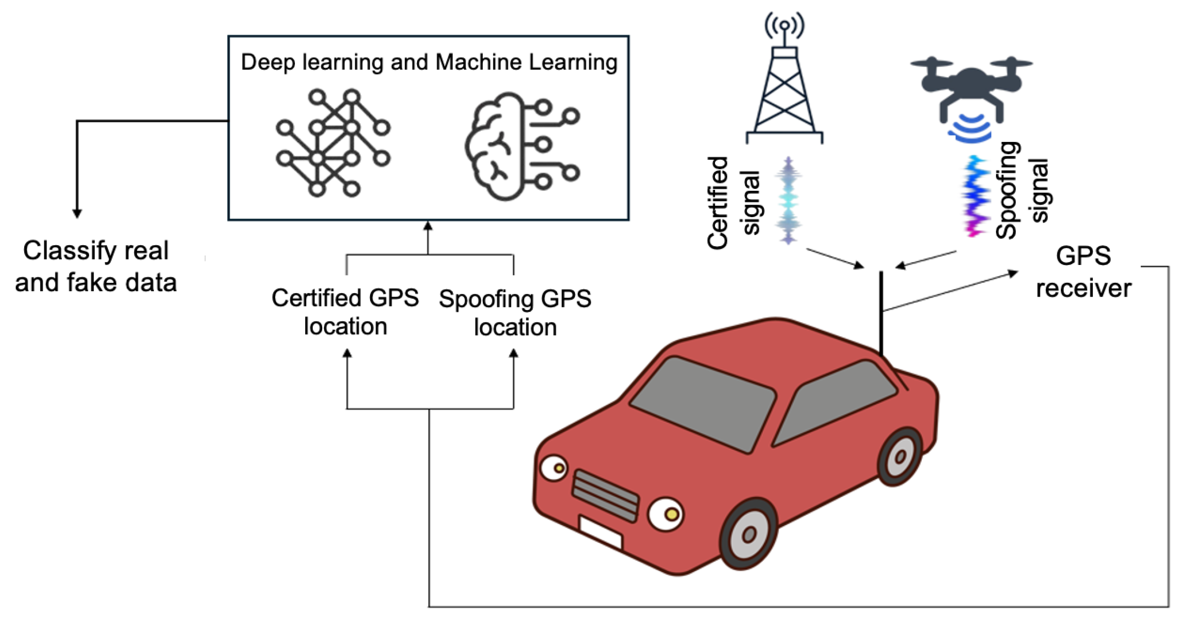
Figure 1.
A GPS spoofing attack launched on a vehicle [
13].
Figure 1.
A GPS spoofing attack launched on a vehicle [
13].
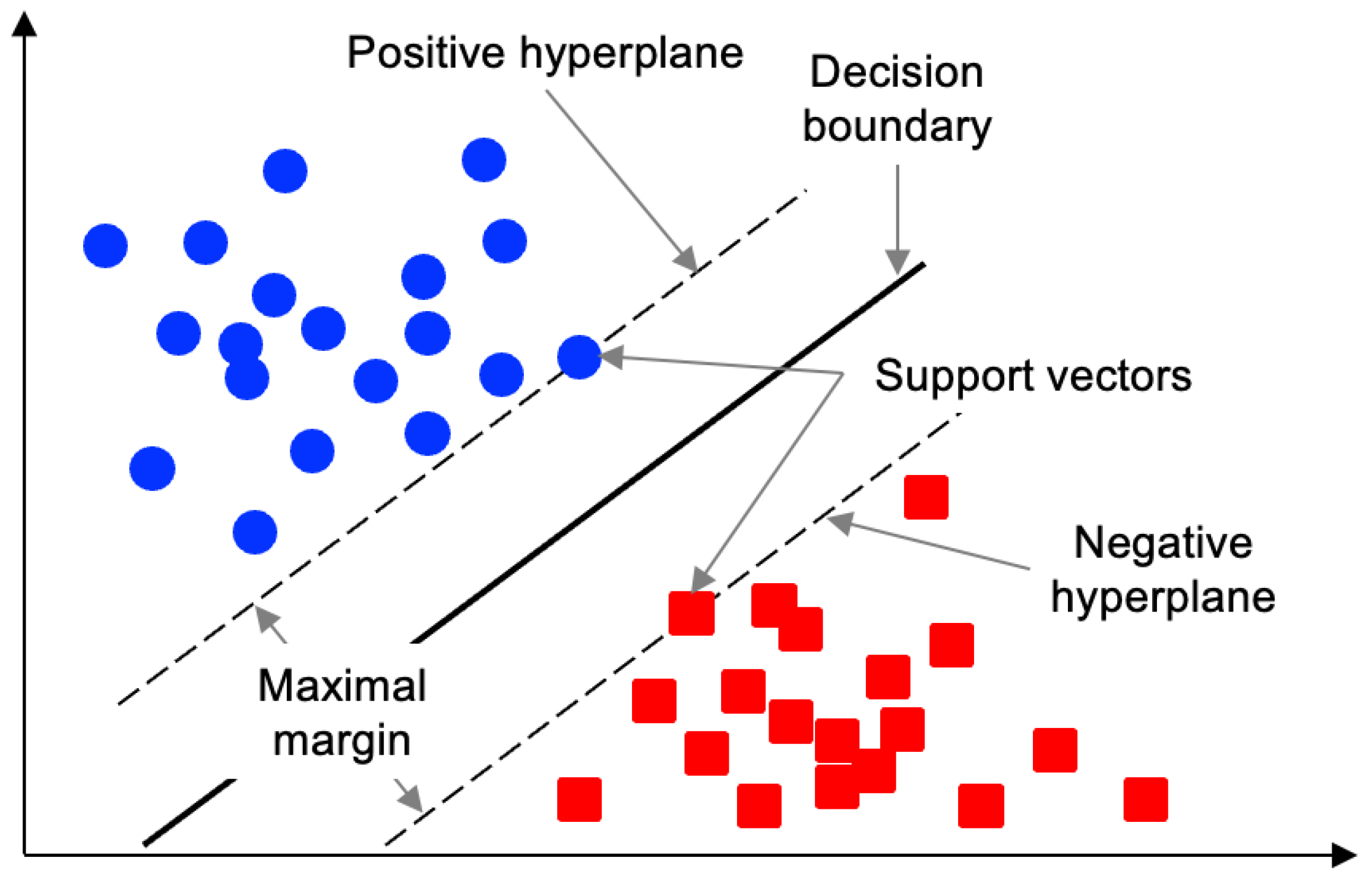
Figure 2.
The support vectors define the margin.
Figure 2.
The support vectors define the margin.
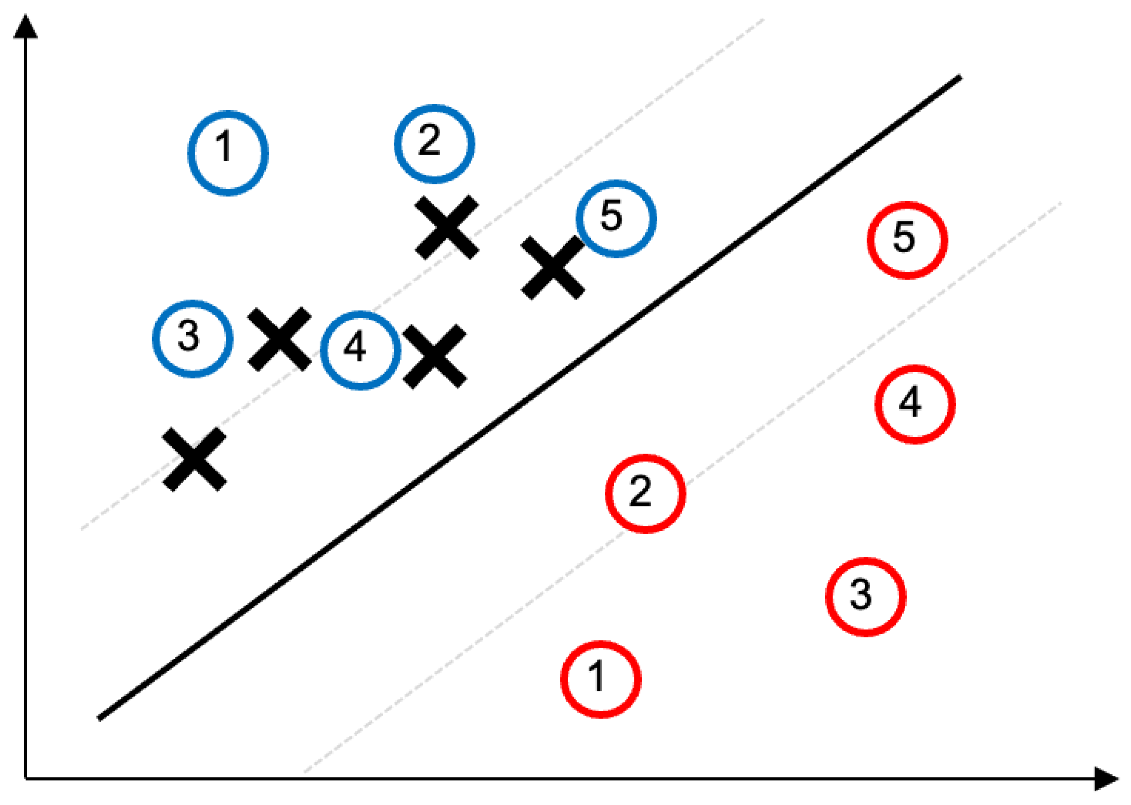
Figure 3.
Schematic of the data location shift attack: the circles represents the true path when there is no attack, which defines the decision boundary (solid line) and two hyperplanes (dashed lines). Under the attack, the vehicle’s perceived path (noted as X) gradually diverges from the true path (blue circles) due to incremental GPS offsets.
Figure 4.
Schematic of the similarity-based noise attack: the overall sequence of small perturbations results in the accumulative noise effect.
Figure 4.
Schematic of the similarity-based noise attack: the overall sequence of small perturbations results in the accumulative noise effect.
Figure 5.
Under the shift attack, the accuracy of the SVM detector gradually decreases as the absolute value of the shift amount [m] increases (from the right side of the x−axis to the left). The average classification accuracy ± standard deviation over 100 runs is reported as follows: 0.999 ± 0.00003, 0.815 ± 0.00029, 0.630 ± 0.00084, 0.445 ± 0.00054, 0.258 ± 0.00046, and 0.204 ± 0.00015.
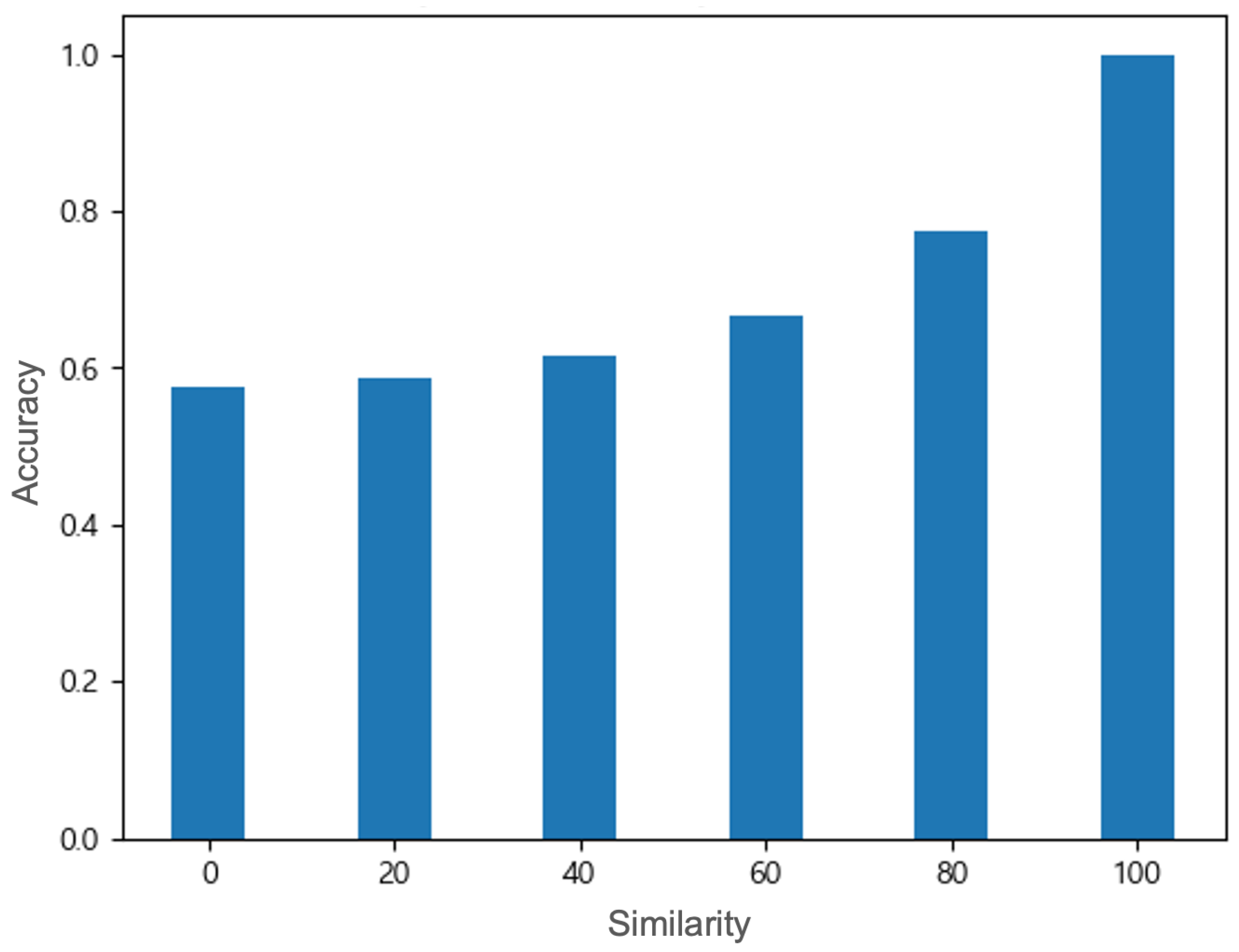
Figure 6.
Under the noise attack, the detector’s accuracy sharply decreases as the similarity [%] decreases; from the right side of the x−axis to the left, the average classification accuracy ± standard deviation over 100 independent runs is 0.999 ± 0.00002, 0.774 ± 0.00024, 0.667 ± 0.00045, 0.616 ± 0.00078, 0.588 ± 0.00073, and 0.574 ± 0.00128.
Figure 7.
Accuracy under combined attacks exhibits a variety of patterns: a nonlinear interaction between shift and noise changes the threshold for classification dynamically. As the similarity increases, two groups of small shifts (−10 and −20) and large shifts (−40 and −50) change in opposite directions.
Figure 8.
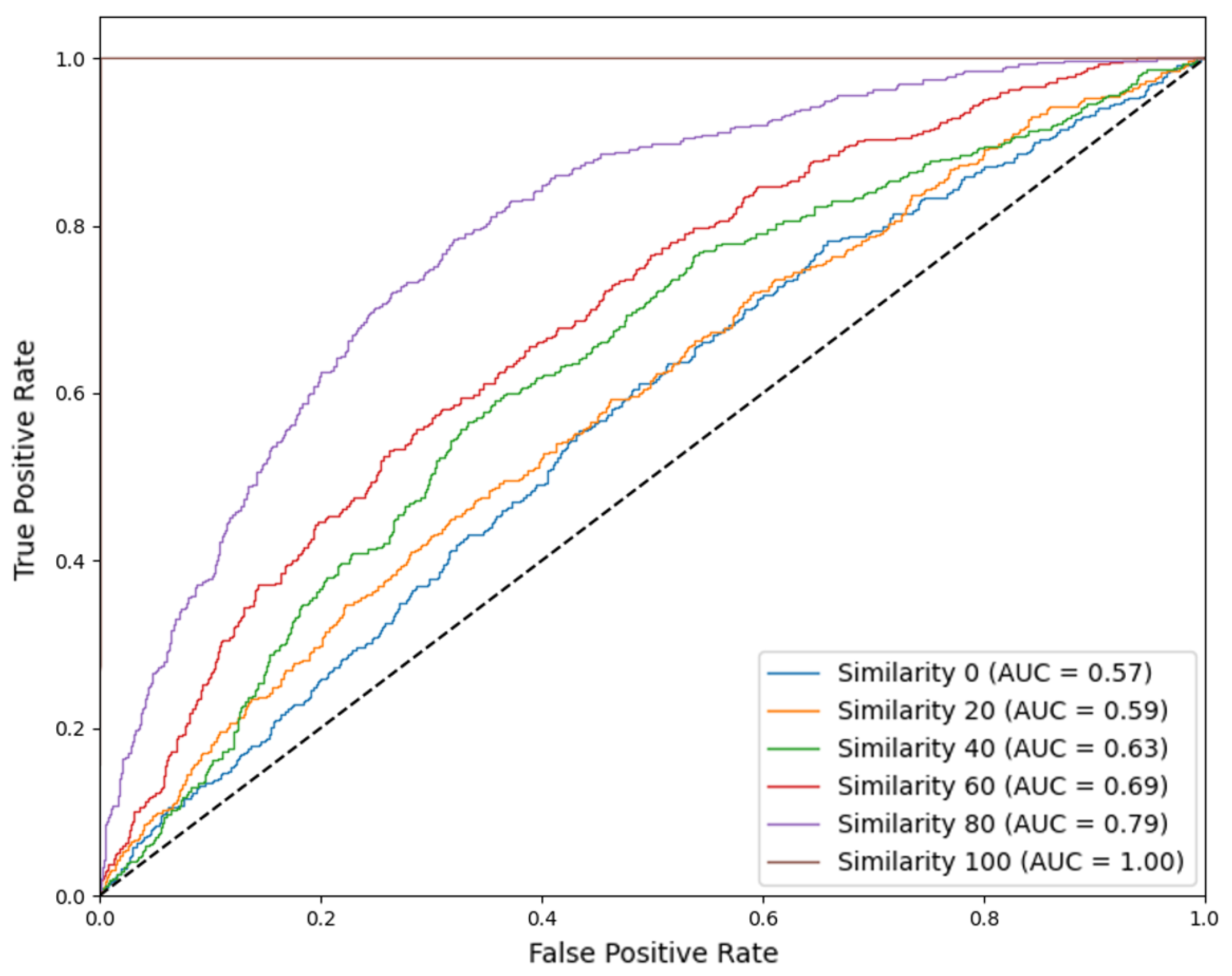
Receiver operating characteristic (ROC) curves for the SVM detector at different similarity levels. In the no-attack scenario (i.e., similarity 100), the AUC achieves 100. As the strength of the attack increases (decreasing similarity), the average value of AUC (over 100 runs) drops to 0.79, 0.69, 0.63, 0.59, and 0.57.
Figure 9.
Under the shift attack, as the absolute value of the shift level decreases (from the left side of the x-axis to the right), the attack becomes more subtle and thus less detectable. The average detection rate (over 100 runs) changes from 0.917 to 0.909, 0.905, 0.892, and 0.872.
Figure 9.
Under the shift attack, as the absolute value of the shift level decreases (from the left side of the x-axis to the right), the attack becomes more subtle and thus less detectable. The average detection rate (over 100 runs) changes from 0.917 to 0.909, 0.905, 0.892, and 0.872.
Figure 10.
Under the noise attack, as the similarity level increases (from the left side of the x-axis to the right), the spoofing noise becomes similar to civilian GNSS error and thus becomes harder to detect. The average detection rate (over 100 runs) changes from 0.478 to 0.469, 0.462, 0.448, and 0.395.
Figure 11.
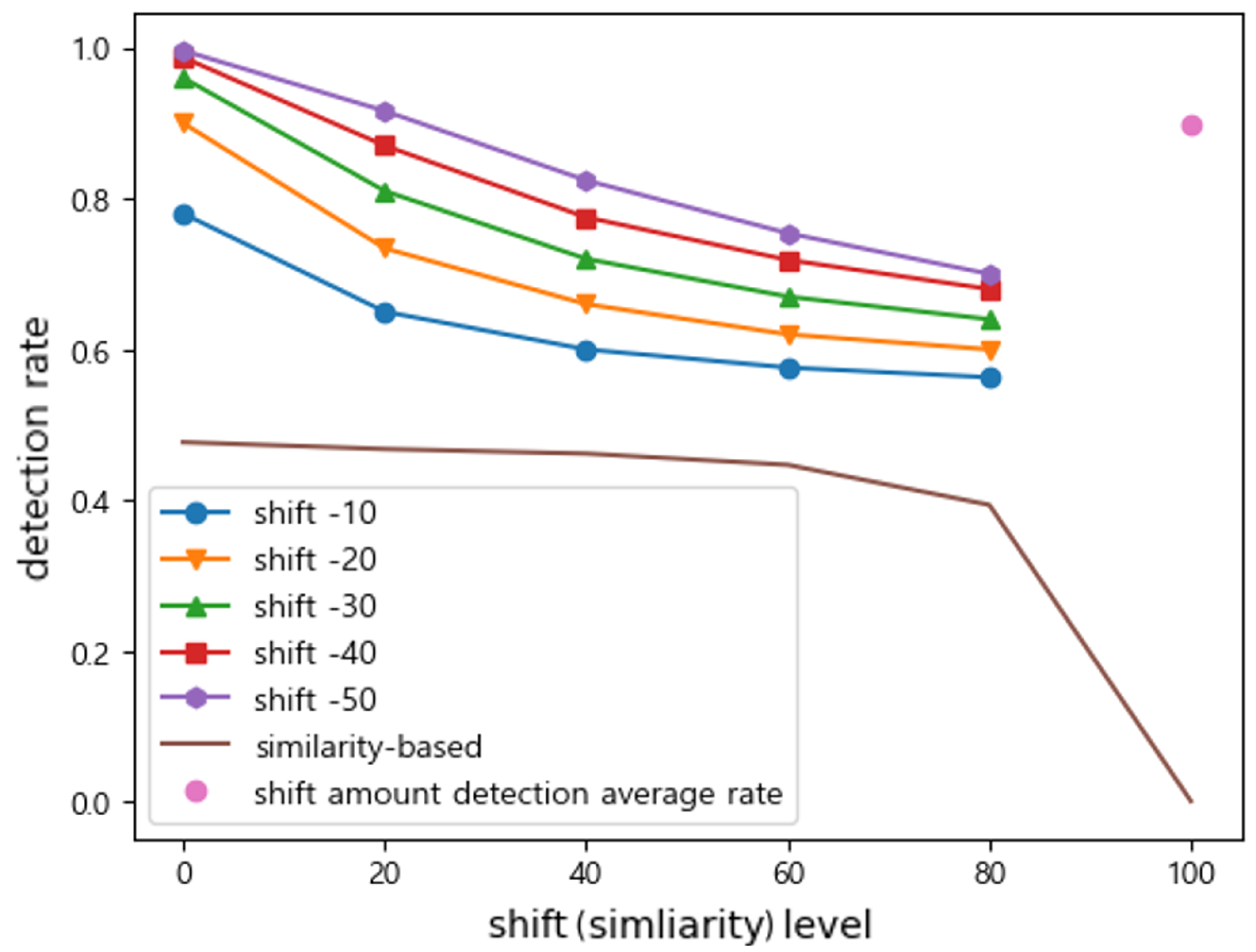
Under the combined attack, the detection rate depends on the balance of shift and noise components. The detection rate is lowered when compared to the shift attack, while we observe a higher detection rate when compared to the noise attack.
Figure 11.
Under the combined attack, the detection rate depends on the balance of shift and noise components. The detection rate is lowered when compared to the shift attack, while we observe a higher detection rate when compared to the noise attack.
Figure 12.
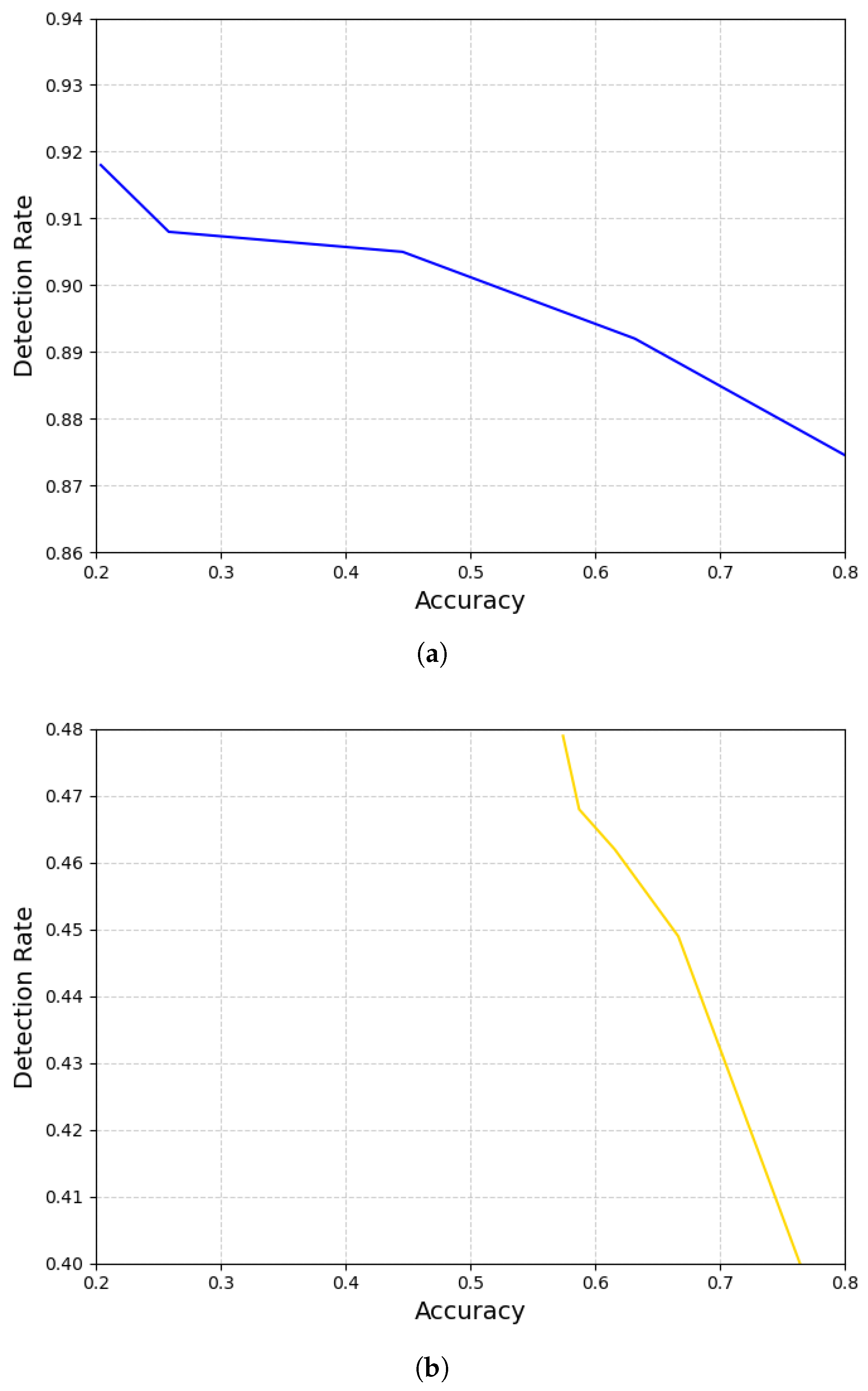
The higher the detection rate, the lower the accuracy. Different attack strategies show different slopes. In the noise attack (
a), the slope is very similar to that in
Figure 9, indicating that the accuracy is almost proportional to the shift amount. However, the slope in the shift attack (
b) is sharper than that in
Figure 10, implying the accuracy is sensitive to the change in the similarity level.
Table 1.
Configurations for CARLA autonomous driving simulation.
Table 1.
Configurations for CARLA autonomous driving simulation.
| CARLA Version | 0.9.15 |
| Map Environment | Town10HD_Opt |
| Vehicle Model | Lincoln MKZ 2020 (default CARLA ego-vehicle) |
| GPS Sensor | Carla.GnssSensor (update rate = 1 Hz) |
| Data Logging | Position and lane offset logged at each time step |
| Control Agent | CARLA Autopilot API |
Table 2.
Parameters and configurations used for experiments.
Table 2.
Parameters and configurations used for experiments.
| Parameter | Setup |
|---|
| Dataset | GPS coordinates from the CARLA driving simulation |
| Number of samples | 10,854 samples in total
- -
80% of samples for training and 20% for testing - -
80% of samples from attack class and 20% from no-attack class.
|
| Number of runs | 100 runs over multiple random seeds |
| Spoofing detection model | SVM with RBF (radial basis function) kernel, linear hyperplane, regularization parameter C = 1.0, gamma = scale |
| Attack scenarios | Shift attack, noise attack, combined attack |
| Maximum offset for Shift | (−50, −40, …, 0) |
| GPS noise model | Gaussian noise, with calibration (noise_lat_stddev = 0.000015 deg and noise_lon_stddev = 0.00002 deg) |
| Noise scaling factor | (0, 20, …, 80) |
| Baseline scenario | No GPS spoofing with autopilot mode |
Table 3.
Classification metrics and confusion matrices for varying shift amounts. A shift amount of 0 represents a no-attack scenario, while −50 denotes the strongest shift attack.
Table 3.
Classification metrics and confusion matrices for varying shift amounts. A shift amount of 0 represents a no-attack scenario, while −50 denotes the strongest shift attack.
| Shift Amount | Precision | Recall | F1-Score | TP | FP | FN | TN |
|---|
| 0 | 0.999 | 0.997 | 0.998 | 2204 | 2 | 7 | 8641 |
| −10 | 0.522 | 0.875 | 0.654 | 1935 | 1772 | 276 | 6871 |
| −20 | 0.355 | 0.900 | 0.510 | 1990 | 3615 | 221 | 5028 |
| −30 | 0.269 | 0.906 | 0.415 | 2003 | 5444 | 208 | 3199 |
| −40 | 0.216 | 0.909 | 0.350 | 2010 | 7295 | 201 | 1348 |
| −50 | 0.204 | 0.919 | 0.333 | 2032 | 7928 | 179 | 715 |
Table 4.
Classification metrics and confusion matrices for varying similarity levels. A similarity of 100 represents a no-attack scenario, while 0 denotes the strongest noise attack.
Table 4.
Classification metrics and confusion matrices for varying similarity levels. A similarity of 100 represents a no-attack scenario, while 0 denotes the strongest noise attack.
| Similarity Level | Precision | Recall | F1-Score | TP | FP | FN | TN |
|---|
| 100 | 0.998 | 0.999 | 0.999 | 2209 | 4 | 2 | 8639 |
| 80 | 0.460 | 0.395 | 0.523 | 873 | 1025 | 1338 | 7618 |
| 60 | 0.319 | 0.447 | 0.404 | 988 | 2110 | 1223 | 6533 |
| 40 | 0.274 | 0.462 | 0.364 | 1021 | 2707 | 1190 | 5936 |
| 20 | 0.254 | 0.468 | 0.344 | 1035 | 3039 | 1176 | 5604 |
| 0 | 0.246 | 0.477 | 0.334 | 1055 | 3233 | 1156 | 5410 |
Table 5.
Average and standard deviation of AUC values across similarity levels.
Table 5.
Average and standard deviation of AUC values across similarity levels.
| Similarity Level | Average AUC | Standard Deviation |
|---|
| 0 | 0.574 | 0.0158 |
| 20 | 0.593 | 0.0225 |
| 40 | 0.630 | 0.0100 |
| 60 | 0.688 | 0.0147 |
| 80 | 0.793 | 0.0094 |
| 100 | 1.000 | 0.0000 |
