Author Contributions
Conceptualization, M.J., P.P. and H.J.; Software, M.J.; Validation, M.J.; Formal analysis, M.J.; Resources, H.J.; Data curation, M.J.; Writing—original draft, M.J.; Writing—review & editing, P.P. and H.J.; Supervision, H.J.; Project administration, H.J.; Funding acquisition, P.P. and H.J. All authors have read and agreed to the published version of the manuscript.
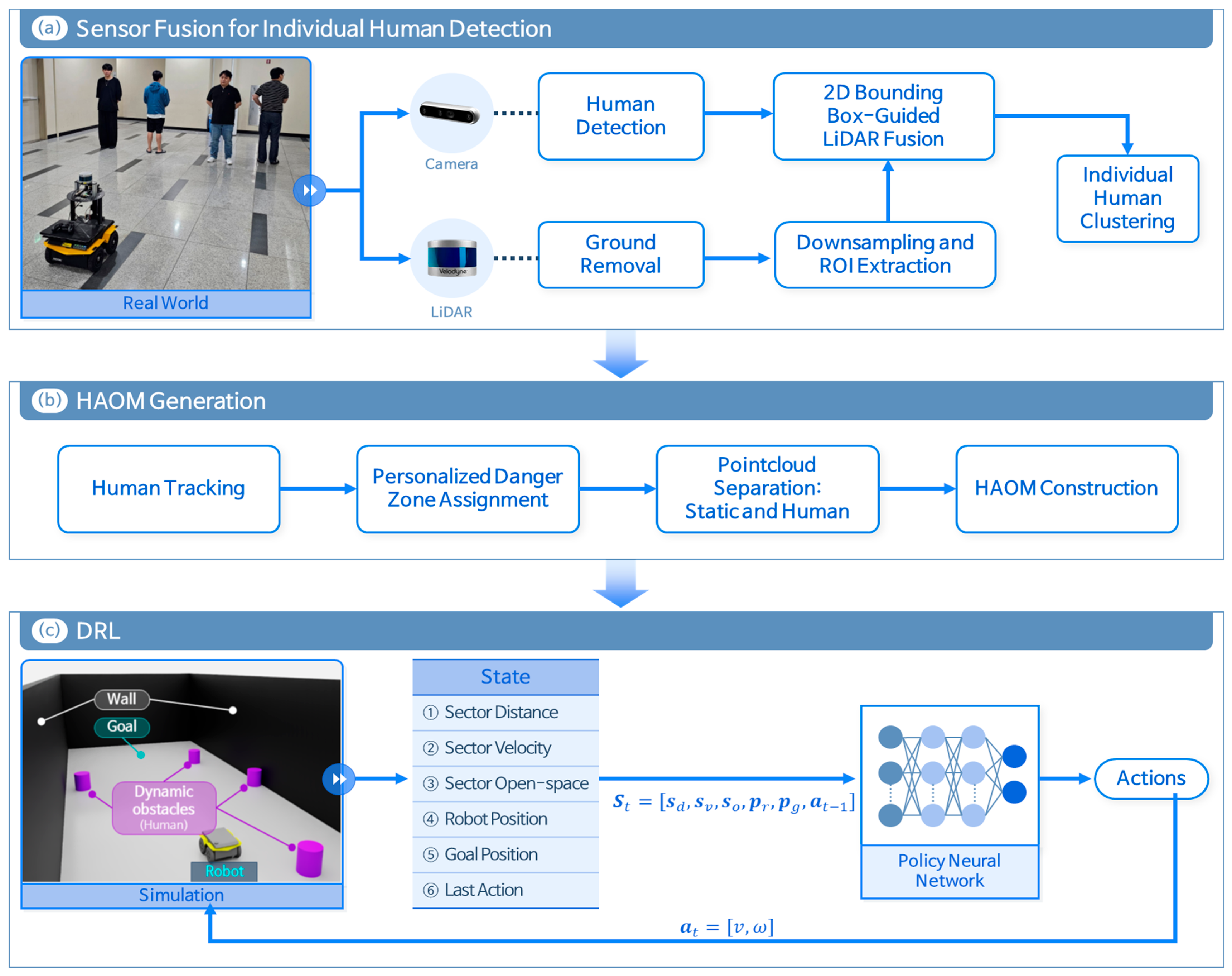
Figure 1.
Architecture of the sensor fusion and deep reinforcement learning (DRL)-based path planning. The mobile robot used was a Clearpath Jackal, equipped with a Velodyne VLP-16 LiDAR and an Intel RealSense D435 camera, running on Ubuntu 20.04 with ROS Noetic.
Figure 1.
Architecture of the sensor fusion and deep reinforcement learning (DRL)-based path planning. The mobile robot used was a Clearpath Jackal, equipped with a Velodyne VLP-16 LiDAR and an Intel RealSense D435 camera, running on Ubuntu 20.04 with ROS Noetic.
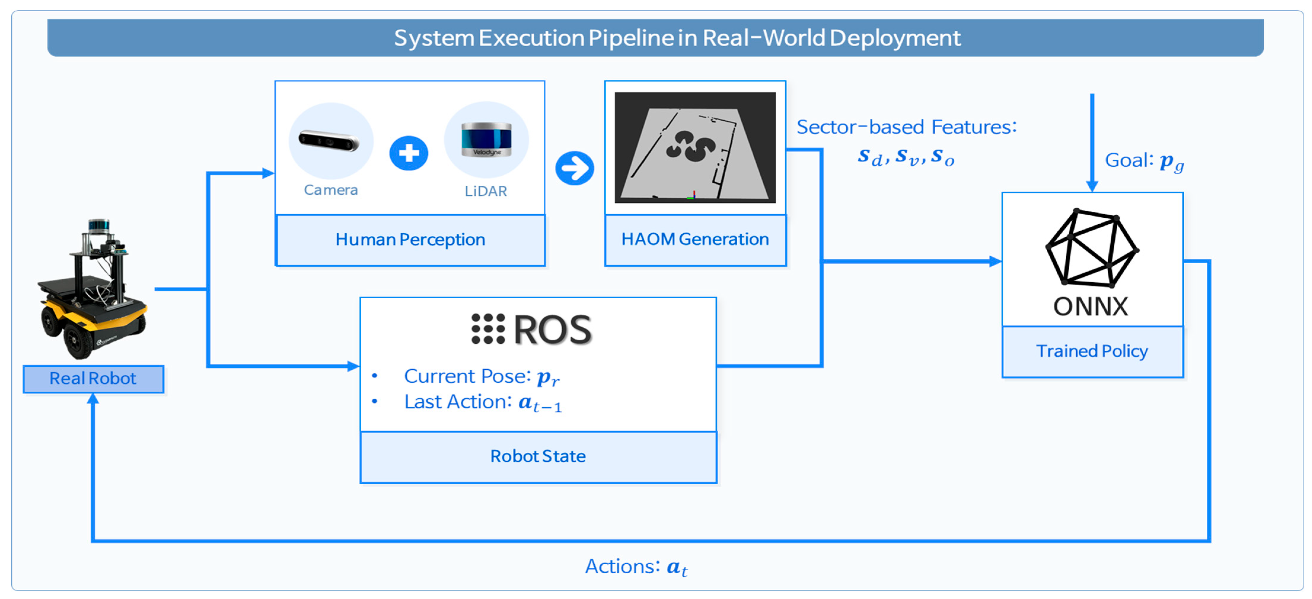
Figure 2.
Real-world execution pipeline of the proposed method.
Figure 2.
Real-world execution pipeline of the proposed method.
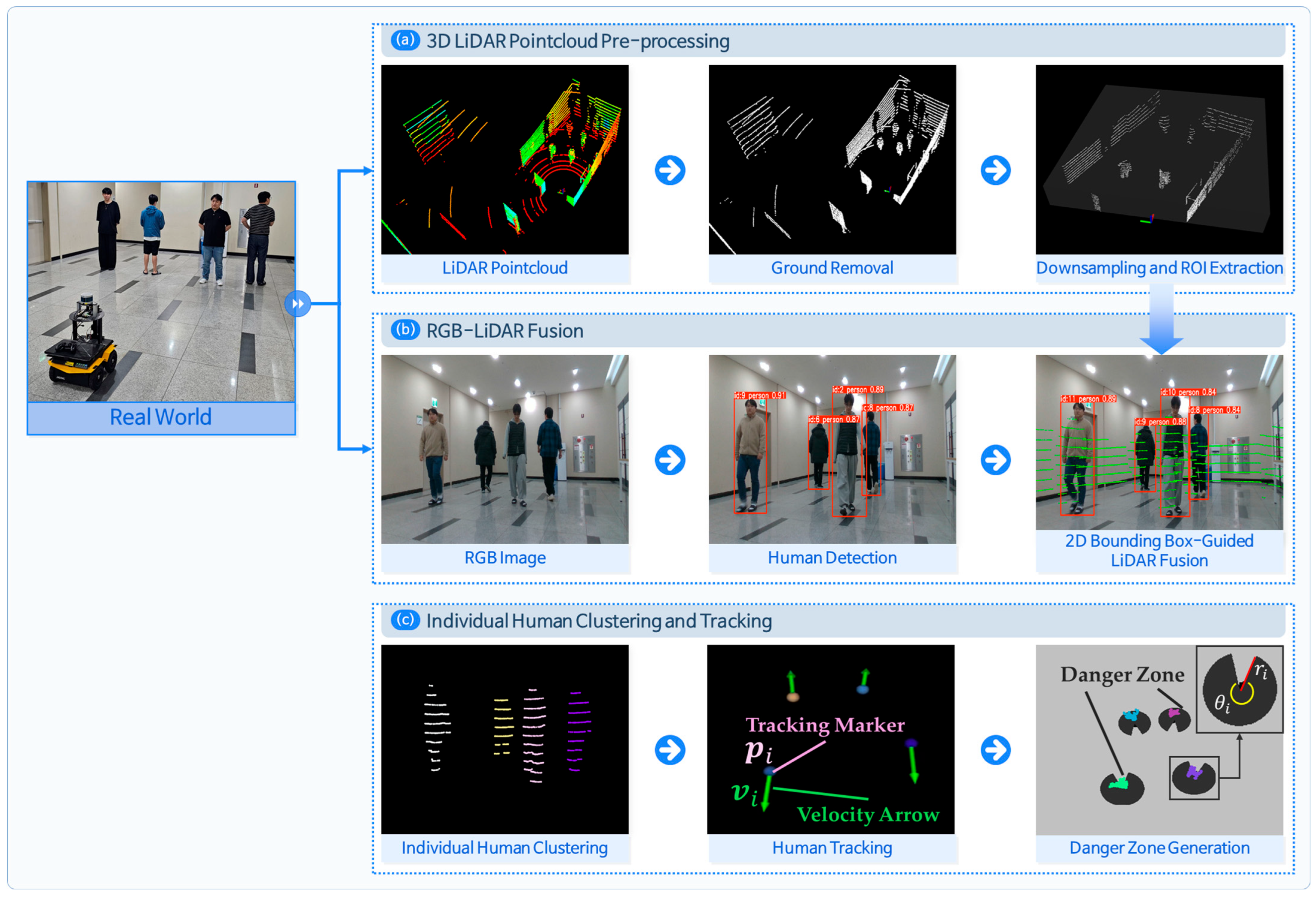
Figure 3.
Sensor fusion pipeline for human-aware navigation. (a) 3D LiDAR preprocessing with ground removal and extracting region of interest (ROI) point cloud; (b) human detection using RGB image and bounding box fusion with LiDAR; and (c) individual-level human clustering with tracking.
Figure 3.
Sensor fusion pipeline for human-aware navigation. (a) 3D LiDAR preprocessing with ground removal and extracting region of interest (ROI) point cloud; (b) human detection using RGB image and bounding box fusion with LiDAR; and (c) individual-level human clustering with tracking.
Figure 4.
Procedure for removing non-pedestrian point clouds.
Figure 4.
Procedure for removing non-pedestrian point clouds.
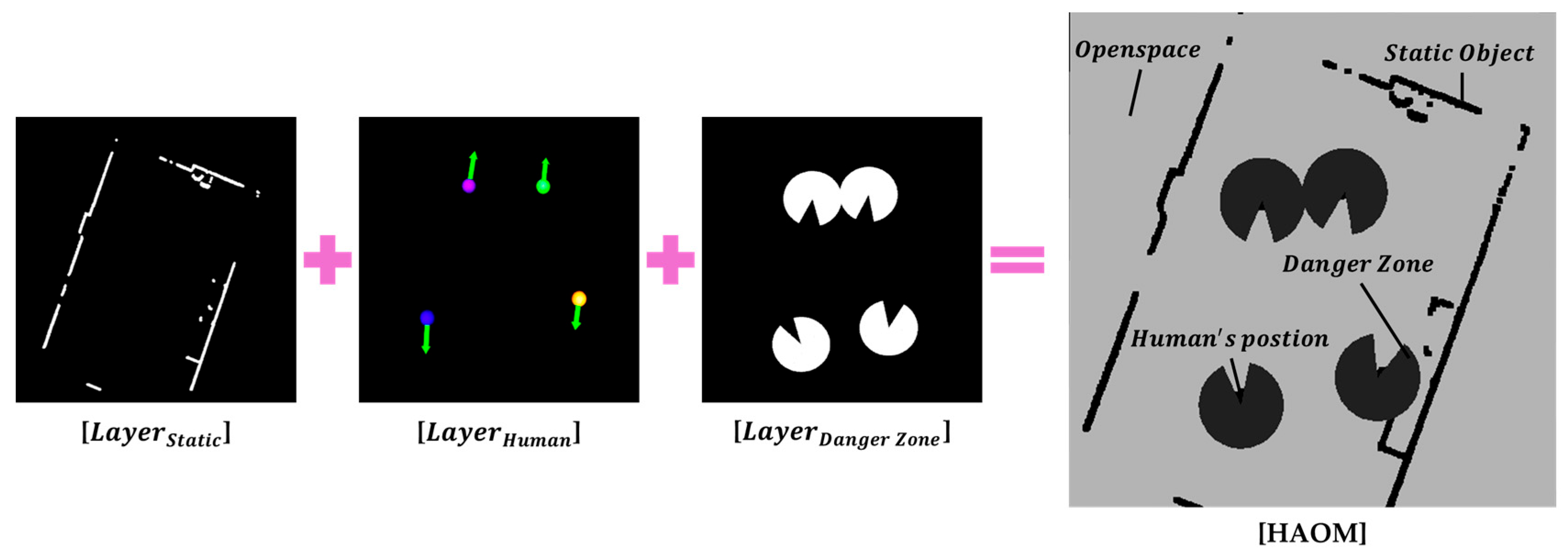
Figure 5.
Human-aware occupancy map (HAOM) comprising static obstacles, centroid positions of pedestrian clusters, dynamic danger zones, and open space.
Figure 5.
Human-aware occupancy map (HAOM) comprising static obstacles, centroid positions of pedestrian clusters, dynamic danger zones, and open space.
Figure 6.
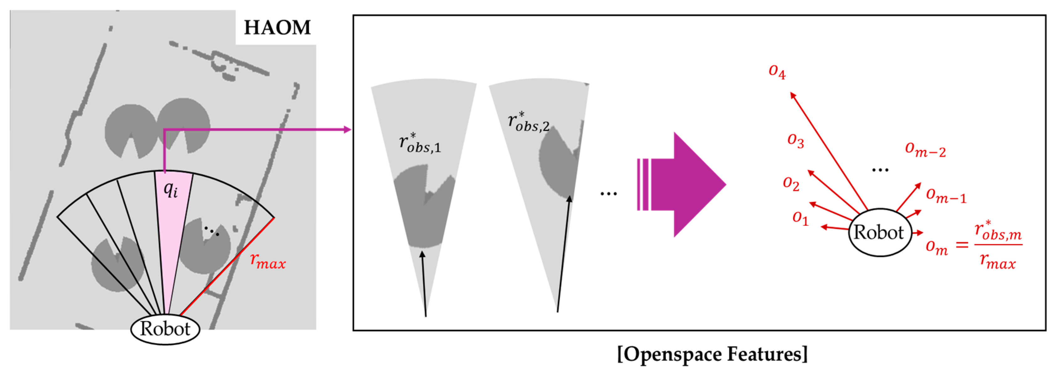
Sector-based distance feature extraction for HAOM. The robot’s front-facing area is divided into n uniform angular sectors . For each sector, the minimum Euclidean distance to static obstacles or the human clusters’ centroid is measured, normalized by the maximum sensing range and encoded as a distance feature .
Figure 7.
Sector-based velocity feature extraction in the camera’s field of view (FOV). The area is evenly divided into angular sectors , and tracked pedestrian positions and velocity vectors are projected into the corresponding sectors.
Figure 7.
Sector-based velocity feature extraction in the camera’s field of view (FOV). The area is evenly divided into angular sectors , and tracked pedestrian positions and velocity vectors are projected into the corresponding sectors.
Figure 8.
Sector-based open-space feature extraction for HAOM in the camera’s FOV. Each angular sector is analyzed to compute the normalized traversable distance considering both static and dynamic obstacles with danger zones.
Figure 8.
Sector-based open-space feature extraction for HAOM in the camera’s FOV. Each angular sector is analyzed to compute the normalized traversable distance considering both static and dynamic obstacles with danger zones.
Figure 9.
Three simulation environments used for performance evaluation. The black represents the wall structures, purple indicates dynamic obstacles, cyan denotes the goal, and gray represents the robot.
Figure 9.
Three simulation environments used for performance evaluation. The black represents the wall structures, purple indicates dynamic obstacles, cyan denotes the goal, and gray represents the robot.
Figure 10.
Visualizations of our method in extreme scenarios: (a) success cases; (b) failure cases. The red line represents the robot’s path.
Figure 10.
Visualizations of our method in extreme scenarios: (a) success cases; (b) failure cases. The red line represents the robot’s path.
Figure 11.
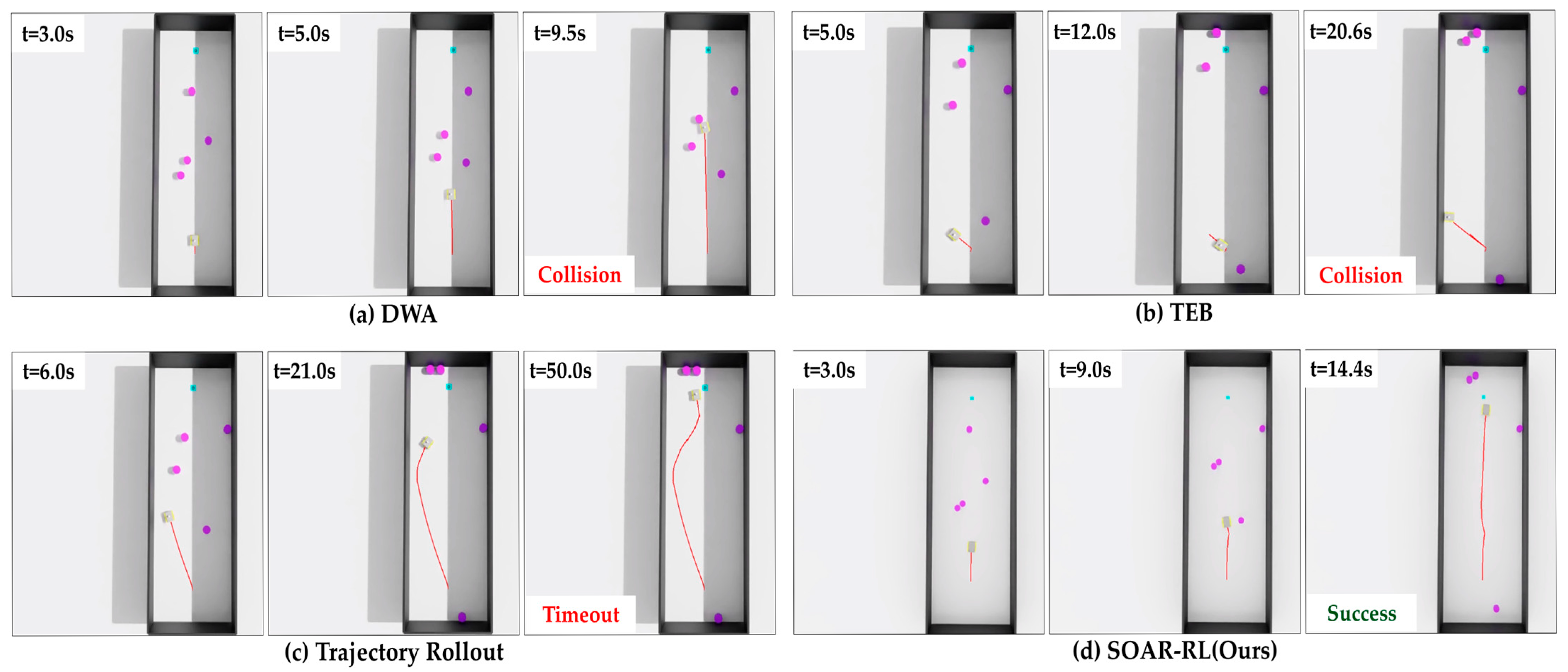
Comparison of navigation trajectories in Scenario 1: (a) dynamic window approach (DWA), (b) timed elastic band (TEB), (c) trajectory rollout (TR), (d) safe and open-space-aware RL (SAOR-RL; ours). The red line represents the robot’s path.
Figure 11.
Comparison of navigation trajectories in Scenario 1: (a) dynamic window approach (DWA), (b) timed elastic band (TEB), (c) trajectory rollout (TR), (d) safe and open-space-aware RL (SAOR-RL; ours). The red line represents the robot’s path.
Figure 12.
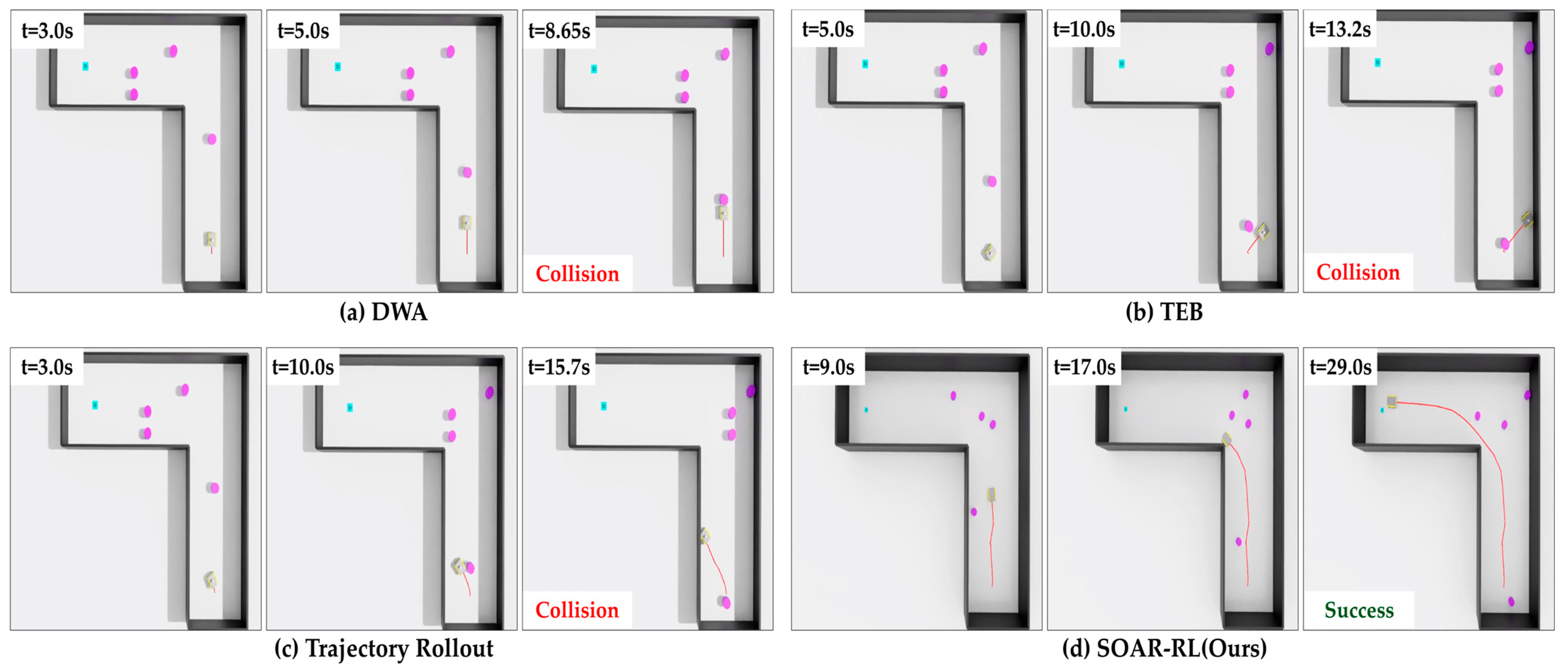
Comparison of navigation trajectories in Scenario 2: (a) dynamic window approach (DWA), (b) timed elastic band (TEB), (c) trajectory rollout (TR), (d) safe and open-space-aware RL (SAOR-RL; ours). The red line represents the robot’s path.
Figure 12.
Comparison of navigation trajectories in Scenario 2: (a) dynamic window approach (DWA), (b) timed elastic band (TEB), (c) trajectory rollout (TR), (d) safe and open-space-aware RL (SAOR-RL; ours). The red line represents the robot’s path.
Figure 13.
Comparison of navigation trajectories in Scenario 3: (a) dynamic window approach (DWA), (b) timed elastic band (TEB), (c) trajectory rollout (TR), (d) safe and open-space-aware RL (SAOR-RL; ours). The red line represents the robot’s path.
Figure 13.
Comparison of navigation trajectories in Scenario 3: (a) dynamic window approach (DWA), (b) timed elastic band (TEB), (c) trajectory rollout (TR), (d) safe and open-space-aware RL (SAOR-RL; ours). The red line represents the robot’s path.
Table 1.
Description of reward functions.
Table 1.
Description of reward functions.
| Reward | Explanation |
|---|
| Arrive: If the robot goal distance is less than , gets . |
| Heading to goal: Measures the cosine similarity between the robot’s current direction and the direction to the goal . If , gets + 1.0. |
| Progress: Calculates the distance reduction to the goal between time steps. |
| Danger zone penalty: Applies a linearly increasing penalty when the robot enters a human’s danger zone [24]. is the robot–obstacles distance; is the danger zone radius. |
| Distance penalty: Penalizes proximity to static obstacles and human danger zones to reduce collision risk. is the open space length in each sector is constant. |
| Open-Dir alignment: Computes the cosine similarity between the robot’s current direction and the central direction vector of the widest open space . |
| Collision penalty: Applies upon collision with obstacles. |
Table 2.
Evaluation metrics used for performance assessment.
Table 2.
Evaluation metrics used for performance assessment.
| Metrics | Explanation |
|---|
| SR | Success rate: Percentage of episodes in which the robot successfully reaches the goal without collisions or timeouts. |
| CR | Collision rate: Percentage of episodes in which the robot collides with any obstacle. |
| TOR | Timeout rate: Percentage of episodes in which the robot fails to reach the goal within the time limit. |
| μR ± σR | Cumulative reward: Mean and standard deviation of cumulative rewards across episodes, indicating overall policy performance. |
| μPL | Path length: Average distance (in meters) the robot travels to reach the goal. |
| μS | Average speed: Average velocity of the robot during successful navigation. |
| NT | Navigation time: Time (in seconds) taken per episode, regardless of whether the robot succeeds, collides, or times out. |
Table 3.
Performance of the proposed method in various environments.
Table 3.
Performance of the proposed method in various environments.
| | Scenario 1 | Scenario 2 | Scenario 3 |
|---|
| # of Dynamic Obstacles | SR (%) | μR ± σR | SR (%) | μR ± σR | SR (%) | μR ± σR |
|---|
| 1 | 98.0 | 157.07 ± 23.68 | 99.0 | 149.39 ± 30.53 | 96.0 | 225.24 ± 39.49 |
| 2 | 95.0 | 145.82 ± 17.89 | 94.0 | 163.76 ± 33.90 | 95.0 | 215.11 ± 40.43 |
| 3 | 91.0 | 147.38 ± 32.53 | 88.0 | 164.84 ± 38.96 | 89.0 | 193.51 ± 32.33 |
| 4 | 87.0 | 144.48 ± 40.17 | 89.0 | 166.86 ± 34.36 | 89.0 | 209.77 ± 32.69 |
Table 4.
Quantitative comparison with and without Open-Dir alignment reward in three scenarios with four dynamic obstacles. Upward ↑ and downward ↓ arrows indicate values that are higher and lower than the value w/o .
Table 4.
Quantitative comparison with and without Open-Dir alignment reward in three scenarios with four dynamic obstacles. Upward ↑ and downward ↓ arrows indicate values that are higher and lower than the value w/o .
| Scenario | Method | SR (%) ↑ | CR (%) ↓ | TOR (%) ↓ | μR ± σR ↑ |
|---|
| Scenario 1 | | 75.0 | 25.0 | 0.0 | 54.51 ± 11.26 |
| w/ | 89.0 | 11.0 | 0.0 | 144.48 ± 40.17 |
| Scenario 2 | | 78.0 | 17.0 | 5.0 | 99.96 ± 25.99 |
| w/ | 93.0 | 7.0 | 0.0 | 166.86 ± 34.36 |
| Scenario 3 | | 75.0 | 19.0 | 6.0 | 138.40 ± 27.41 |
| w/ | 91.0 | 5.0 | 4.0 | 209.77 ± 32.69 |
Table 5.
Quantitative performance comparison of the proposed method and traditional navigation methods with four dynamic obstacles. Upward ↑ and downward ↓ arrows indicate values that are higher and lower than the result of traditional navigation methods.
Table 5.
Quantitative performance comparison of the proposed method and traditional navigation methods with four dynamic obstacles. Upward ↑ and downward ↓ arrows indicate values that are higher and lower than the result of traditional navigation methods.
| Scenario | Method | SR (%) ↑ | CR (%) ↓ | TOR (%) ↓ | μPL (m) ↑ | μS (m/s) ↑ | NT (s) |
|---|
| Scenario 1 | DWA [13] | 39.0 | 45.0 | 16.0 | 4.92 | 0.48 | 10.26 |
| TEB [14] | 32.0 | 48.0 | 20.0 | 4.42 | 0.46 | 11.83 |
| TR [32] | 49.0 | 13.0 | 38.0 | 8.38 | 0.34 | 22.73 |
| SOAR-RL (Ours) | 93.0 | 7.0 | 0.0 | 9.43 | 0.66 | 14.39 |
| Scenario 2 | DWA [13] | 36.0 | 48.0 | 16.0 | 3.26 | 0.38 | 12.64 |
| TEB [14] | 35.0 | 47.0 | 18.0 | 3.89 | 0.41 | 15.17 |
| TR [32] | 48.0 | 21.0 | 31.0 | 4.63 | 0.38 | 30.78 |
| SOAR-RL (Ours) | 94.0 | 6.0 | 0.0 | 15.10 | 0.61 | 25.27 |
| Scenario 3 | DWA [13] | 42.0 | 45.0 | 13.0 | 6.54 | 0.41 | 14.24 |
| TEB [14] | 41.0 | 33.0 | 26.0 | 4.51 | 0.46 | 21.87 |
| TR [32] | 49.0 | 14.0 | 37.0 | 9.88 | 0.37 | 37.57 |
| SOAR-RL (Ours) | 88.0 | 12.0 | 0.0 | 20.99 | 0.61 | 34.03 |
Table 6.
Quantitative performance comparison of the proposed method and crowd navigation methods with five dynamic obstacles. Upward ↑ and downward ↓ arrows indicate values that are higher and lower than the result of AI-based crowd navigation methods.
Table 6.
Quantitative performance comparison of the proposed method and crowd navigation methods with five dynamic obstacles. Upward ↑ and downward ↓ arrows indicate values that are higher and lower than the result of AI-based crowd navigation methods.
| Method | SR (%) ↑ | CR (%) ↓ | TOR (%) ↓ | μPL (m) ↓ | μS (m/s) | NT (s) ↓ |
|---|
| ORCA [33] | 31.0 | 68.0 | 1.0 | 2.91 | 0.35 | 8.41 |
| CADRL [34] | 78.0 | 16.0 | 6.0 | 4.49 | 0.56 | 8.04 |
| LSTM-RL [35] | 89.0 | 8.0 | 3.0 | 7.05 | 0.87 | 8.10 |
| DSRNN [36] | 93.0 | 7.0 | 0.0 | 10.01 | 1.02 | 9.78 |
| SOAR-RL (Ours) | 94.0 | 6.0 | 0.0 | 4.21 | 0.61 | 5.28 |
Table 7.
Runtime performance summary across different navigation scenarios.
Table 7.
Runtime performance summary across different navigation scenarios.
| Scenarios | Avg. FPS |
|---|
| Scenario 1 | 24.03 |
| Scenario 2 | 24.53 |
| Scenario 3 | 24.24 |
| Scenario 4 | 21.19 |
