1. Introduction
There are many important real-world applications that rely on adaptive filters [
1,
2,
3]. Such popular signal processing tools are frequently involved in system identification problems [
4], interference cancellation schemes [
5], channel equalization scenarios [
6], sensor networks [
7], and prediction configurations [
8], among many others. The key block that controls the overall operation of this type of filter is the adaptive algorithm, which basically commands the coefficients’ update.
There are several families of adaptive filtering algorithms, among which two stand out as the most representative [
1,
2,
3]. First, the least-mean-square (LMS) algorithms are popular due to their simplicity and practical features, especially in terms of low computational complexity. However, their performance is quite limited when operating with highly correlated input signals and/or long-length filters. The second important category of algorithms belong to the recursive least-squares (RLS) family, with improved convergence performance as compared to their LMS counterparts, even in the previously mentioned challenging scenarios. Nevertheless, the RLS algorithms are more computationally expensive and can also experience some stability problems in practical implementations. On the other hand, the performance of implementation platforms nowadays is exponentially improving, in terms of both processing speed and implementation facility. Consequently, the popularity of the RLS-type algorithms is also constantly growing, thus becoming the solution of choice in different frameworks [
9,
10,
11].
Motivated by these aspects, the current paper targets further improvements on the global performance of the RLS algorithm, by aiming for a better control of its convergence parameters. The application framework focuses on the system identification problem, which represents one of the basic configurations in adaptive filtering, with a wide range of applications [
2]. In this context, the forgetting factor represents one of the main parameters that tune the algorithm behavior [
3]. This positive subunitary constant weights the square errors that contribute to the cost function, so that it mainly influences the memory of the algorithm. A larger value of this parameter (i.e., closer to one) leads to a better accuracy of the solution provided by the adaptive filter. However, in order to remain alert to any potential changes in the system to be identified, a lower value of the forgetting factor is desired, which would lead to a faster tracking reaction.
The RLS algorithm should also be robust to different external perturbations in the operating environment, which can frequently happen in system identification scenarios. For example, let us consider an echo cancellation context [
5], where an acoustic sensor (i.e., microphone) captures the background noise from the surroundings, which can be significantly strong and highly nonstationary. In this case, the algorithm should be robust to such variations, a goal that cannot be achieved using only the forgetting factor as the control parameter. Toward this purpose, the cost function of the algorithm should include (besides the error-related term) an additional regularization component [
12,
13,
14,
15]. As a result, the robustness of the algorithm is controlled in terms of the resulting regularization parameter. Nevertheless, most of the regularized RLS algorithms require additional (a priori) information about the environment or need some extra parameters that are difficult to evaluate in practice. Moreover, a robust behavior to such external perturbations (related to the environment) is usually paid by a slower tracking reaction when dealing with time-varying systems.
These conflicting requirements, in terms of accuracy, tracking, and robustness, lead to a performance compromise between these main performance criteria. More recently, the data-reuse technique was also introduced and analyzed in the context of RLS algorithms [
16,
17,
18]. The basic idea is to use the same set of data (i.e., the input and reference signals) several times within each main iteration of the algorithm, in order to improve the convergence rate and the tracking capability of the filter. Usually, mainly due to complexity reasons, the date-reuse method is extensively used in conjunction with LMS-type algorithms [
19,
20,
21,
22,
23,
24,
25,
26]. The solutions proposed in [
16,
18], in the framework of RLS-type algorithms, replace the multiple iterations of the data-reuse process with a single equivalent step, thus maintaining the computational complexity order of the original algorithm. Moreover, the data-reuse parameter (i.e., the number of equivalent data-reuse iterations) is used as an additional control factor, in order to improve the tracking capability of the RLS algorithm, even when operating with a large value of the forgetting factor.
The previous work [
16] introduced the data-reuse principle in the context of the conventional RLS algorithm, which does not include any regularization component within its cost function, so that it is inherently limited in terms of robustness. Following [
16], a convergence analysis of this algorithm was presented in [
17]. More recently, we developed a data-reuse regularized RLS algorithm [
18], with improved robustness features, where the regularization parameter is related to the signal-to-noise ratio (SNR). The current work represents an extension of the conference paper [
18], with a twofold new contribution. First, it provides additional theoretical details and simulation results related to the algorithm developed in [
18], also including a practical estimation of the SNR. Second, it presents a novel regularization technique recently proposed in [
27], in conjunction with the data-reuse technique, thus resulting in a new RLS-type algorithm. Its regularization parameter considers both the influence of the external noise and a term related to the model’s uncertainties. This approach leads to improved performance as compared to the previously developed data-reuse regularized RLS algorithm.
Following this introduction, the rest of this paper is structured as follows.
Section 2 contains the basics of the regularized RLS algorithms, including the recent method from [
27]. Next,
Section 3 develops the data-reuse method in conjunction with the regularized RLS algorithms. Simulation results are presented in
Section 4, in the framework of echo cancellation. The paper is concluded in
Section 5, which summarizes the main findings and outlines several perspectives for future research.
2. Regularized RLS Algorithms
Let us consider a system identification setup [
3] having the reference (or desired) signal, obtained as
where
n represents the discrete-time index,
is a vector containing the most recent
L samples of the zero-mean input signal
, with the superscript
T denoting the transpose of a vector or a matrix,
is the impulse response (of length
L) of the system that we need to identify, and
is a zero-mean additive noise signal, which is independent of
. In this context, the main objective is to identify
with an adaptive filter, denoted by
Therefore, the a priori error between the reference signal and its estimate results in
where
represents the output of the adaptive filter. In the framework of echo cancellation [
5], a replica of the echo signal is obtained at the output of the adaptive filter. In other words, the echo path impulse response is estimated/modeled by the adaptive filter, so that this unknown system (i.e., the echo path) is identified. Thus, the echo cancellation application can be formulated as a system identification problem.
This system identification problem can be solved following the least-squares (LS) optimization criterion [
3], which is based on the minimization of the cost function:
where
is the forgetting factor, with
. This parameter controls the memory of the algorithm, as explained in
Section 1. The minimization of
with respect to
leads to the normal equations [
3]:
where
The estimates from (
5) and (
6) are associated, respectively, to the covariance matrix of the input signal, and to the cross-correlation vector between the input and reference sequences. The system of equations from (
4) can be recursively solved, thus leading to the conventional RLS algorithm [
3], which is defined by the update
The standard initialization of this algorithm is
and
, where
and
denote an all-zero vector of length
L and the identity matrix of size
, respectively, while
is a positive constant, also known as the regularization parameter. However, the influence of
is only limited to the initial convergence of the algorithm, since its contribution is diminishing when
n increases, due to the presence of the subunitary forgetting factor
. As we can notice from (
5), when using the previous initialization for
, the matrix
contains the term
, which is basically negligible for
n large enough and
. As a result, the overall performance of the conventional RLS algorithm, in terms of accuracy and tracking, is basically influenced by the forgetting factor, which represents the main control parameter. On the other hand, these performance criteria are conflicting, since a large value of
(i.e., close to one) leads to a good accuracy of the filter estimate, but with a slow tracking reaction (when the system changes). In order to improve the tracking behavior, the forgetting factor should be reduced, while sacrificing the accuracy of the solution. In terms of robustness (against external perturbations), the higher the value of
, the more robust the algorithm is. However, there is an inherent performance limitation even for
, so that using the forgetting factor as the single control mechanism is not always a practical asset.
As outlined in
Section 1, the robustness of RLS-type algorithms can be improved by incorporating a proper regularization component directly into the cost function. There are different approaches to this problem; however, the practical issues should also be taken into account. In other words, the resulting regularization term should be easy to control in practice, without requiring additional or a priori knowledge related to the system or the environment. Among the existing solutions, we present in the following two practical regularization techniques.
The first one involves the Euclidean norm (or the
regularization), so that the cost function of the regularized RLS algorithm [
1] results in
where
denotes the Euclidean norm. In this case, the update of the regularized RLS algorithm becomes
In order to find a proper value of
, the solution proposed in [
12] rewrites the update from (
9) as
where
In this way, we can notice a “separation” in the right-hand side of (
10), where
depends only on the input signal, while
represents the correctiveness component of the algorithm. In relation to this component, a new error signal can be defined as
At this point, in order to attenuate the effects of the noise in the estimate from (
12), the condition imposed in [
12] is to find
in such a way that
where
stands for mathematical expectation and
is the variance of the noise signal from (
1). Developing (
14) based on (
12), the regularization parameter results in [
12]
where
represents the signal-to-noise ratio, while
and
are the variances of the output signal and the input sequence, respectively. It can be noticed from (
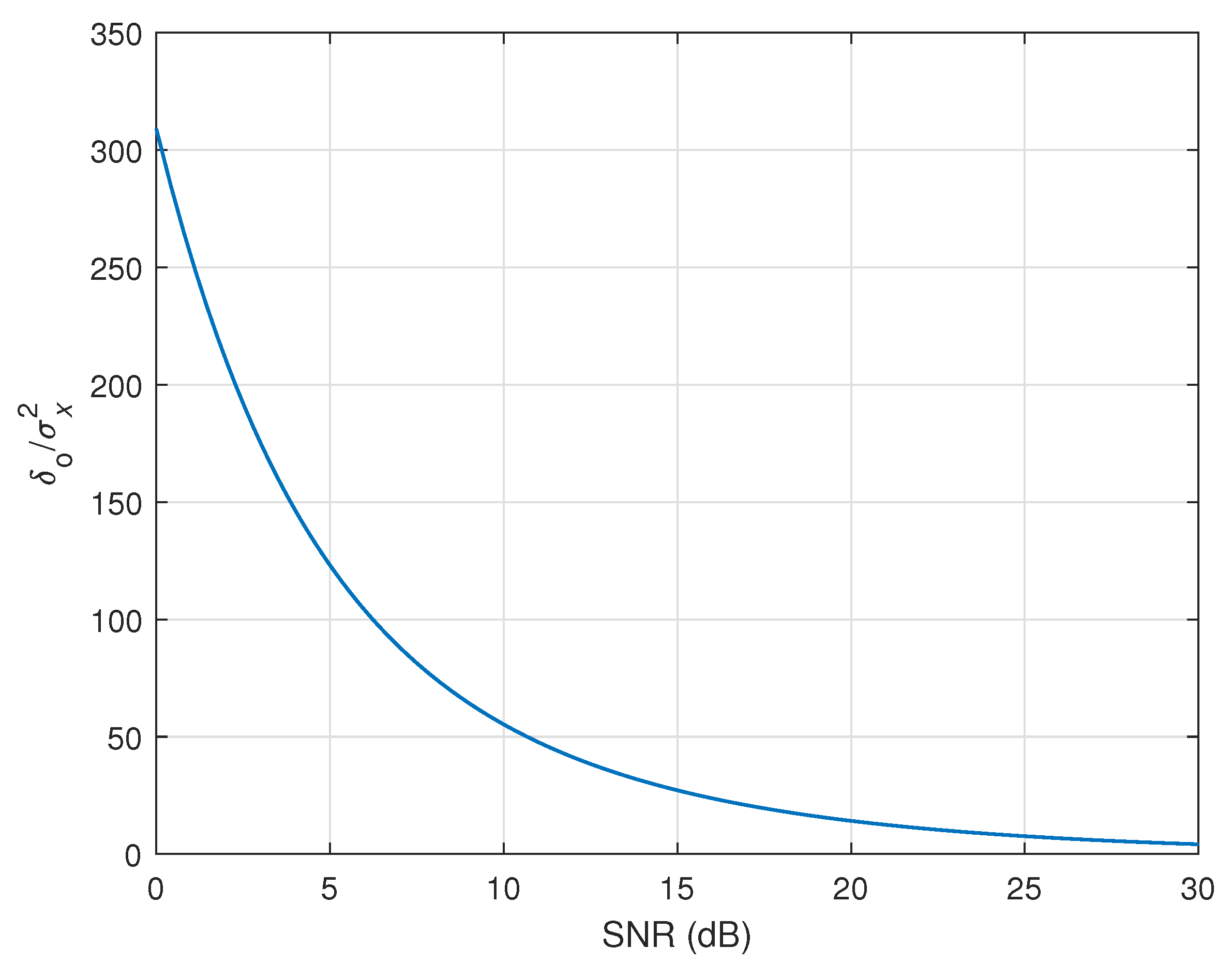
15) that a low SNR leads to a high value of
and, consequently, to a small update term in (
9), which is the desired behavior in terms of robustness in noisy conditions. Nevertheless, in practice, the SNR is not available and should be estimated.
A simple yet efficient method to this purpose was proposed in [
13]. It relies on the assumption that the adaptive filter has converged to a certain degree, i.e.,
, so that
, where
denotes the variance of the estimated output from the right-hand side of (
2). Also, since
and
are uncorrelated, taking the expectation in (
1) results in
where
is the variance of the reference signal. Therefore,
, so that the SNR can be approximated as
where the absolute value at the denominator is used to prevent any minor deviations of the estimates (which could make the SNR negative) and
is a very small positive constant that prevents a division by zero. Since the signals required in (
17) are available, i.e.,
and
, their associated variances can be recursively estimated as
where the forgetting factor
is now used as a weighting parameter. The initialization is
. The resulting algorithm defined by the update (
9), which uses
computed based on (
15) and using the estimated SNR from (
17), is referred to as the variable-regularized RLS (VR-RLS) algorithm [
13].
The second practical regularization technique analyzed in this work has been recently proposed in [
27]. It considers a linear state model, where the observation equation is given in (
1), while the state system follows a simplified first-order Markov model:
where
is a zero-mean white Gaussian noise signal vector, which is uncorrelated to
and
. Related to this model, we denote by
and
the variance and covariance matrix of
, respectively. The first-order Markov model is frequently used for modeling time-varying systems (or nonstationary environments), especially in the context of adaptive filters [
1,
2,
3]. Moreover, this model fits very well for echo cancellation scenarios [
5], where the impulse response of the echo path (to be modeled by the adaptive filter) is associated to a time-varying system, which can be influenced by several factors. For example, in acoustic echo cancellation, the room impulse response is influenced by temperature, pressure, humidity, and the movement of objects or bodies. Thus, the model in (
20) represents a benchmark in this framework in order to model the unknown dynamics of the environment. In this context, it represents a particularly convenient stochastic model for such time-varying systems. This model represents systems that gradually change into an unpredictable direction, which is strongly in agreement with the nature of time-varying impulse responses of the echo paths.
Next, in order to find the estimate
, the weighted LS criterion is used, together with a regularization term that incorporates the model uncertainties, which are captured by
. Consequently, the cost function is
This cost function takes into consideration both types of noise, i.e., the external noise that corrupts the output of the system and the internal noise that models the system uncertainties. In (
21), the first term consists of the standard RLS cost function from (
3), which is weighted by the external noise power (
), while the second term consists of a weighted sum (using the same forgetting factor
) of the terms that contain the covariance matrix of
in order to capture the model uncertainties (
).
The minimization of
with respect to
leads to a set of normal equations that can be recursively solved using the update [
27]:
where
The second term from the right-hand side of (
23) can be interpreted as the noise-to-uncertainty ratio (NUR) and captures the effects of both “noises,” i.e., the external perturbation and the model uncertainties, which are related to the environment conditions and system variability, respectively. Clearly, the NUR is unavailable in practice and should be estimated. The solution proposed in [
27] uses the following recursive estimators for the main parameters required in (
23):
using the same forgetting factor
as a weighting parameter. The initialization is
and
, where the small positive constant
is used since the estimate from (
25) appears at the denominator of (
23).
The estimator from (
24) is based on the fact that in system identification scenarios, the goal of the adaptive algorithm is not to drive the error signal to zero, since this would introduce noise into the filter estimate. Instead, the noise signal should be recovered from the error of the adaptive filter after this one converges to its steady-state solution. In other words, some related information about
can be extracted from the error signal,
. Second, the estimator from (
25) is derived based on (
20). Thus, using the adaptive filter estimates from time indices
n and
, we can use the approximation
, while
, for
. In this way, the term
captures the uncertainties in the system. In summary, the resulting regularized RLS algorithm based on the weighted LS criterion, referred to as WR-RLS [
27], is defined by the update (
22), with the regularization parameter
evaluated as in (
23), and using the estimated NUR based on (
24) and (
25).
3. Data-Reuse Regularized RLS Algorithms
The general update of the regularized RLS algorithms presented in the previous section can be summarized as follows:
where
and
generally denotes the regularization parameter, which can be a positive constant or a variable term that can be evaluated, as in (
15) or (
23). The filter update from (
26) is performed for each set of data, i.e.,
and
, and for each time index
n. On the other hand, in the context of the data-reuse approach, this process is repeated
N times for the same time index
n, i.e., the same set of data is reused
N times. As a result, for the regularized RLS algorithms, the relations that define the data-reuse are
Since
[or
] depends only on
, it remains the same within the cycle associated with the data-reuse process. It can be noticed that the conventional regularized RLS algorithm from (
26) is obtained when
.
Nevertheless, it is not efficient (especially in terms of computational complexity) to implement the data-reuse process in the conventional way, as presented before. As an equivalent alternative, we show in the following how the entire data-reuse cycle can be efficiently grouped into a single update of the filter. Let us begin with the first step, which can be written as
The previous relations are then involved within the second step, which can be developed as
using the notation:
It was also taken into account that
, due to the specific symmetry of the matrix
. Therefore, in this second step, we can evaluate the update of the filter as
Similarly, the third step of the data-reuse process becomes equivalent to
Following the same approach and using mathematical induction, we obtain the relations associated with the final
Nth step of the cycle, i.e.,
It is known that
,
,
, and
sums the
N terms of a geometric progression with the common ratio
. The later term can be computed as
so that the final update becomes
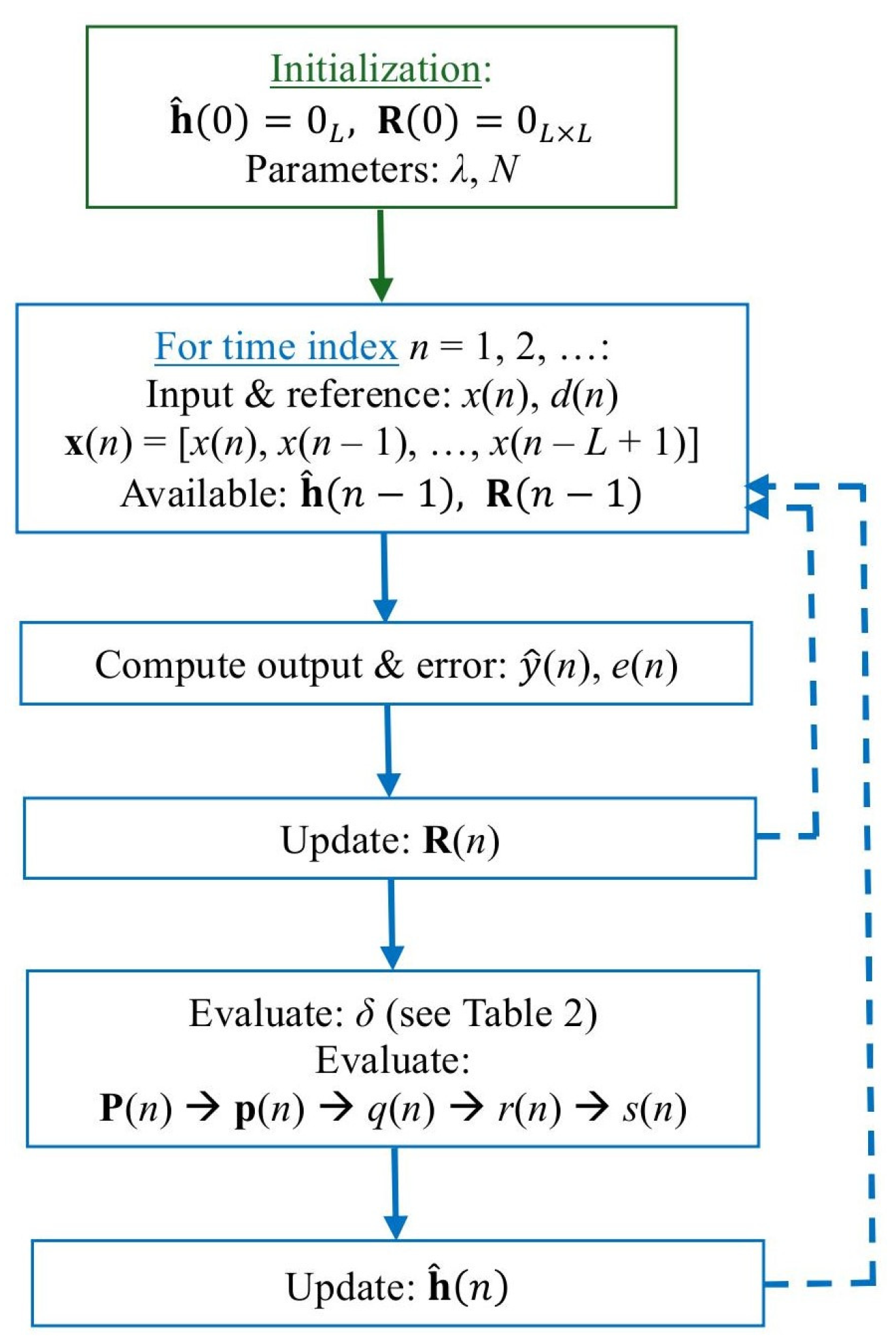
The resulting data-reuse regularized RLS algorithm is summarized in
Table 1 in a slightly modified form, which targets a more efficient implementation. Also, a block diagram of this type of algorithm is presented in
Figure 1. The most challenging operations (in terms of complexity) are the matrix inversion and the computation of
. However, these steps could be efficiently solved using line search methods, like the conjugate gradient (CG) or coordinate descent (CD) algorithms [
28,
29,
30]. (These methods have not been considered here for the implementation of the data-reuse regularized RLS-type algorithms, since they are beyond the scope of this paper. However, they represent a subject for future work, as will be outlined in
Section 5). Also, the update of
can be computed by taking into account the symmetry of this matrix and the time-shift property of the input vector,
. Thus, only the first row and column should be computed, while the rest of the elements are available from the previous iteration. As compared to the conventional regularized RLS algorithm, there is only a moderate increase in terms of computational complexity, mainly due to the evaluation of
. Nevertheless, this extra computational amount is reasonable, i.e.,
L multiplications and
additions.
The data-reuse parameter
N can play the role of an additional control factor, besides the forgetting factor
. In this context, we aim to improve the overall performance of the algorithm, even when using a very large value of
(i.e., very close or equal to 1), which leads to a good accuracy, but significantly affects the tracking. As a consequence, the data-reuse regularized RLS algorithm can attain a better compromise between the main performance criteria, i.e., accuracy versus tracking. Moreover, using a proper regularization parameter for this type of algorithm, like in (
15) or (
23), can improve its behavior in noisy environments.
The regularization parameter of the data-reuse regularized RLS algorithm can be set or evaluated in different ways, as indicated in
Table 2. In the simplest approach,
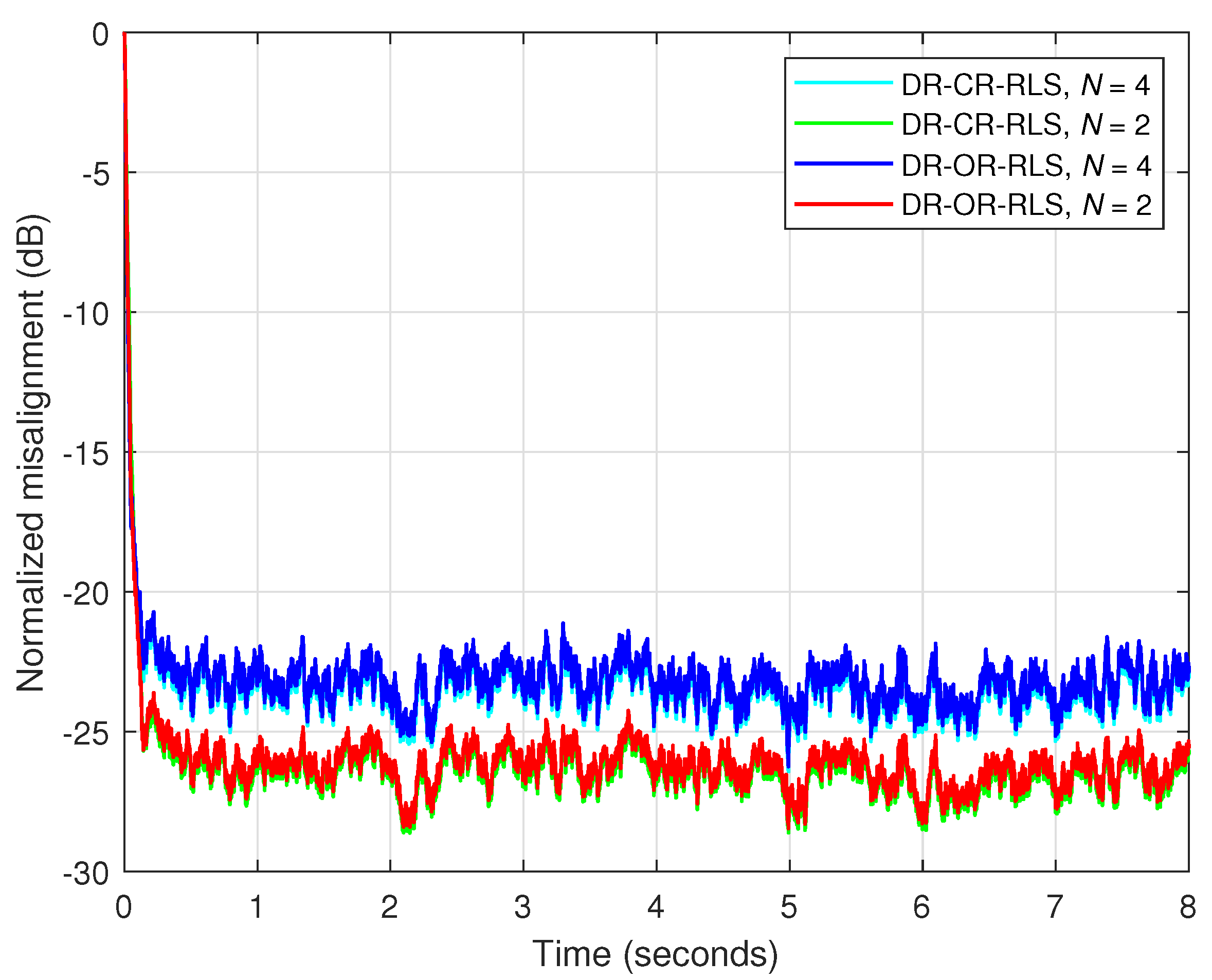
is selected as a positive constant, thus resulting in the data-reuse conventionally regularized RLS (DR-CR-RLS) algorithm. A more rigorous method for setting the constant regularization parameter relies on its connection to the SNR [
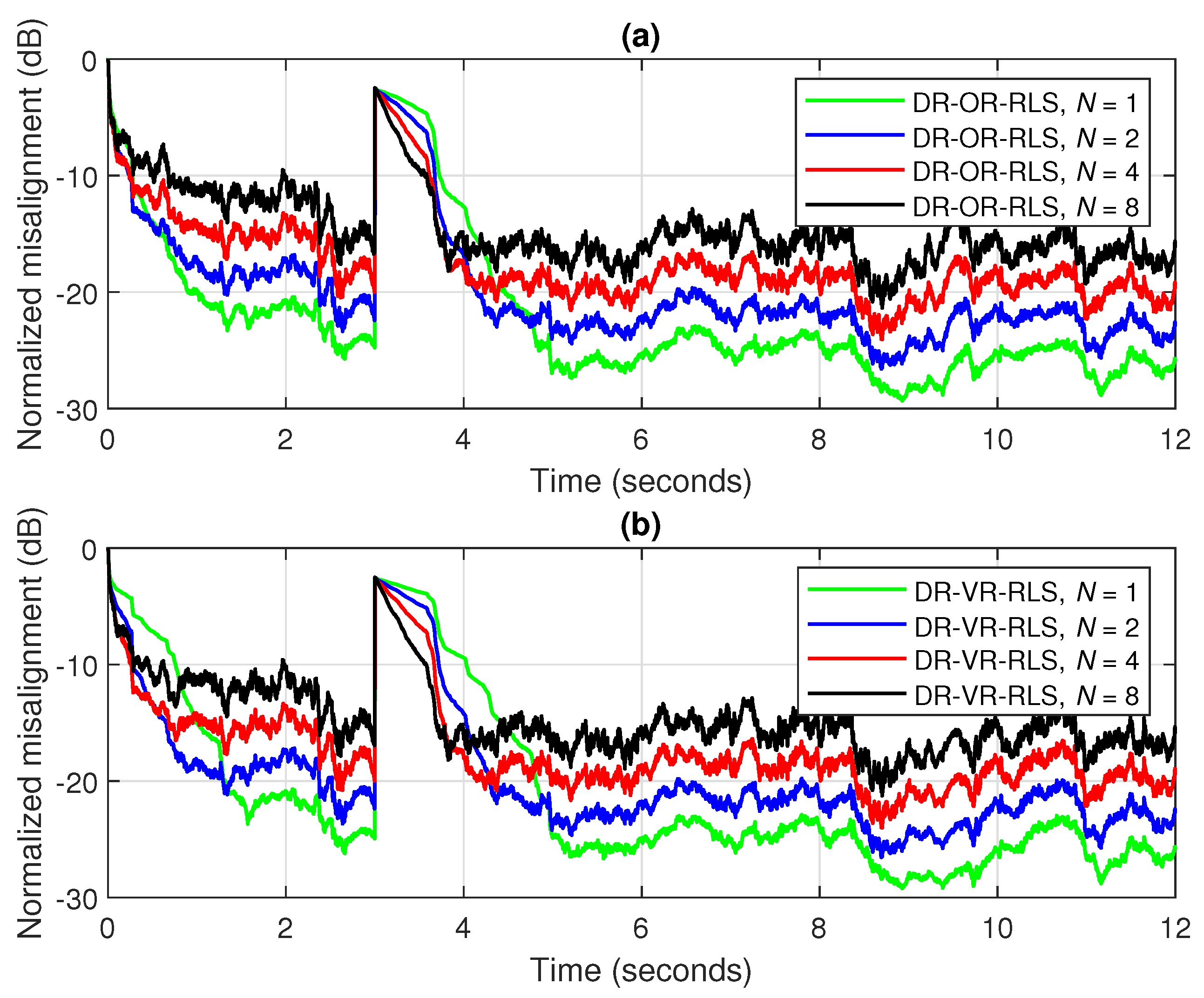
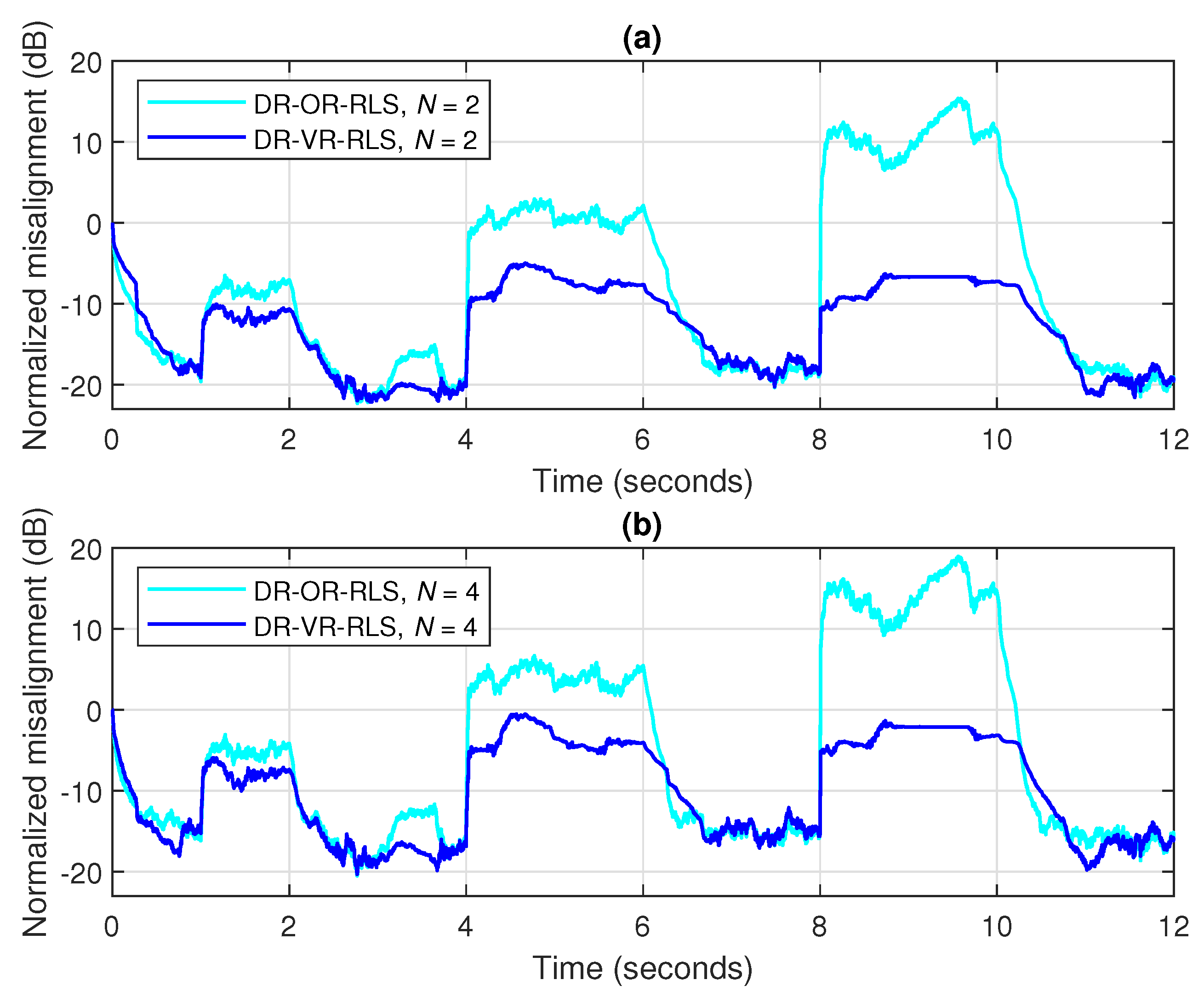
12]. In conjunction with the data-reuse technique, this led to the data-reuse optimally regularized RLS (DR-OR-RLS) presented in [
18].
Nevertheless, the estimated SNR from (
17) was not considered in [
18], where the true value of the SNR was assumed to be available in the evaluation of the “optimal” regularization constant,
(see
Table 2). As an extension to this previous work, the estimated SNR from (
17) is considered in the current paper. Here, the parameter
from (
15) is used within the matrix
from (
41), but it is evaluated based on (
17), in conjunction with (
18) and (
19). The resulting algorithm is referred to as the data-reuse variable-regularized RLS (DR-VR-RLS) algorithm. For
, it is equivalent to the VR-RLS algorithm from [
13].
The regularization parameter specific to the WR-RLS algorithm [
27], i.e.,
from (
23), can also be involved within the matrix
. Thus, in conjunction with the previously developed data-reuse process, which led to the update (
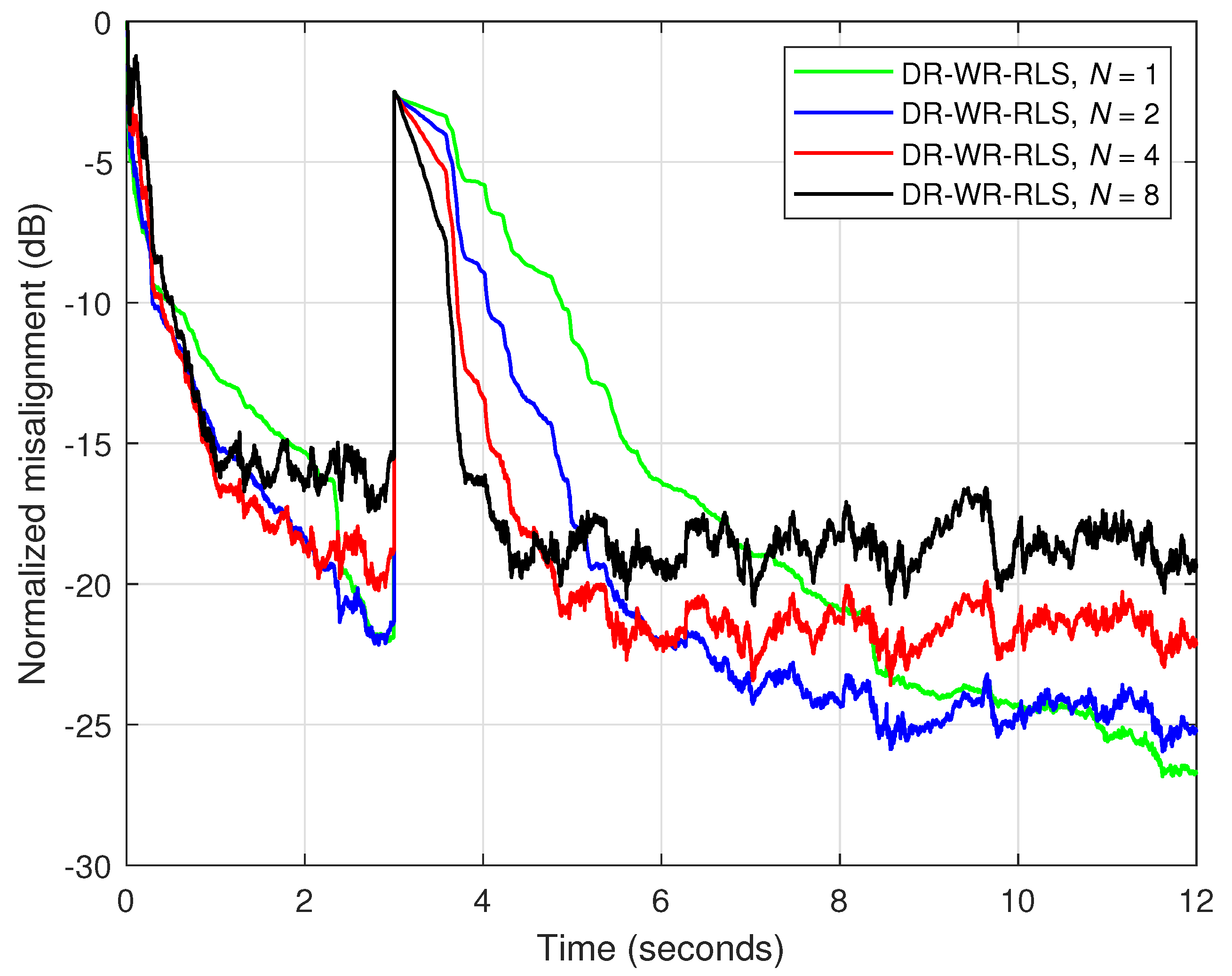
41), a data-reuse WR-RLS (DR-WR-RLS) algorithm is obtained. Its regularization relies on (
23), while using the estimated NUR based on (
24) and (
25). Also, the WR-RLS algorithm from [
27] is a special case obtained when
.
As compared to the DR-VR-RLS algorithm that relies only on the estimated SNR, the regularization approach behind the DR-WR-RLS algorithm is potentially better, since it also includes the contribution of the model uncertainties within the NUR. In other words, the NUR can represent a better measure (for robustness control) instead of the SNR. For both DR-VR-RLS and DR-WR-RLS algorithms, their regularization parameters are time-dependent, so that the time index is indicated in
Table 2, for
and
, respectively.
The computational complexity of these data-reuse regularized RLS algorithms is provided in
Table 3 (in terms of the number of multiplications per iteration), as compared to the standard RLS and LMS algorithms [
1,
2,
3]. Clearly, the LMS algorithm is the least complex, since its update is similar to (
7), but using a positive constant
(known as the step-size parameter) instead of
. However, it is known that the overall performance of the LMS algorithms (in terms of both the convergence rate and accuracy of the estimate) is inferior to the RLS-based algorithms, especially when operating with long-length filters and correlated input signals [
1,
2,
3]. The complexity order of the RLS-based algorithms is proportional to
, but it also depends on the computational amount required by the matrix inversion, which is denoted by
in
Table 3. The conventional RLS algorithm avoids this direct operation by using the matrix inversion lemma [
3], so that its complexity order remains proportional to
. There are several alternative (iterative) techniques that can be used in this context, for solving the normal equations related to the RLS-based algorithms. Among the existing solutions, the dichotomous coordinate descent (DCD) method [
28] represents one of the most popular choices, since it reduces the computational amount up to
, using a proper selection of its parameters. Nevertheless, the influence of these methods on the overall performance of the algorithms is beyond the scope of this paper and it will be investigated in future works (as will be outlined later in
Section 4.6). The evaluation of the regularization parameter of the DR-⋆R-RLS algorithms from
Table 2 (where ⋆ generally denotes the corresponding version, i.e., C/O/V/W), denoted by
, requires only a few operations, as compared to the overall amount. For example, in case of the DR-CR-RLS and DR-OR-RLS algorithms, the regularization parameters can be set a priori. The DR-VR-RLS requires only 6 multiplications per iteration for evaluating
, while the computational amount related to
of the DR-WR-RLS algorithm is
multiplications per iteration. Even if the DR-WR-RLS algorithm is the most complex among its counterparts from
Table 2, its improved performance compensates for this extra computational amount, as will be supported in
Section 4. Also, since
, the computational amount required by the data-reuse process is negligible in the context of the overall complexity of the data-reuse regularized RLS algorithms. In addition, their robustness features justify the moderate extra computational amount as compared to the standard RLS algorithm.
Finally, we should outline that a detailed theoretical convergence analysis of the proposed algorithms is a self-containing issue that is beyond the scope of the paper and it will be explored in future works. Nevertheless, at the end of this section, we provide a brief convergence analysis in the mean value, under some simplified assumptions. First, let us consider that the covariance matrix of the input signal is close to a diagonal one, i.e.,
. Consequently, for large enough
n, its estimate from (
5) results in
. Also, for
(like in echo cancellation scenarios), the approximation
is valid. At this point, let us note that a general rule for setting the forgetting factor is [
18]
with
. Under these circumstances, based on (
27) and (
34), we obtain
Since
, it can be noticed that
and
can be considered as deterministic, being obtained as the sum of a geometric progression with
N terms and the common ratio
. At the limit, when
(i.e.,
), the common ratio becomes
, which results in
.
Next, we assume that the system to be identified is time-invariant, so that its impulse response is fixed (for the purpose of this simplified analysis), i.e.,
. In this context, the system mismatch (or the coefficients’ error) can be defined as
, so that the condition for the convergence in the mean value results in
, for
. This is equivalent to
, for
, which implies that the coefficients of the adaptive filter converge to those of the system impulse response. Based on (
1) and (
2), the update from (
41) can be developed as
so that subtracting
from both sides (and changing the sign), an update for the system mismatch is obtained as
Then, taking the expectation on both sides of (
46), using (
43), and considering that
(since the input signal and the additive noise are uncorrelated), we obtain
As indicated in
Table 1, the initialization for the adaptive filter is
, so that
. Hence, processing (
47)—starting with this initialization—results in
Thus, to obtain the exponential decay toward zero, the convergence condition translates into
. Using the upper limit
, which, as explained before, is related to (
44), we need to verify that
. Since
, we have
, so that we basically need to verify that
, i.e.,
. This condition is always true in practice, since the common setting is
. Consequently, the data-reuse regularized RLS algorithm is convergent in the mean value.
In addition, a simple and reasonable mechanism to evaluate the stability of the algorithm is related to the conversion factor [
1,
3]. First, similarly to (
2) but using the coefficients from the time index
n, we can define the a posteriori error of the adaptive filter as
Next, using the updated (
41) in (
49) and taking (
2) into account, we obtain
where
represents the so-called conversion factor. Under the same simplified assumptions used before (related to the convergence in the mean), this conversion factor can be approximated as
For stability, we need to verify that
, which further leads to
. Since the second term from the right-hand side of (
52) is positive, the condition
is always true. In order to also have
, the ratio from (
52) should be subunitary, i.e.,
. Thus, using
is sufficient to fulfill this condition and to guarantee the stability of the algorithm. This represents a common practical setting in most of the scenarios, as shown in the next section.
