1. Introduction
The current vibration monitoring systems face several limitations, including the susceptibility of the site and oil analysis to the environmental and installation space constraints, the complexity of the signal transmission path, and the difficulty of extracting wear particles. Moreover, the acoustic signals are prone to environmental interference and may be insensitive to certain faults and other issues. Therefore, new technologies and methods for the effective online monitoring of the wear states of mechanical systems are urgently required.
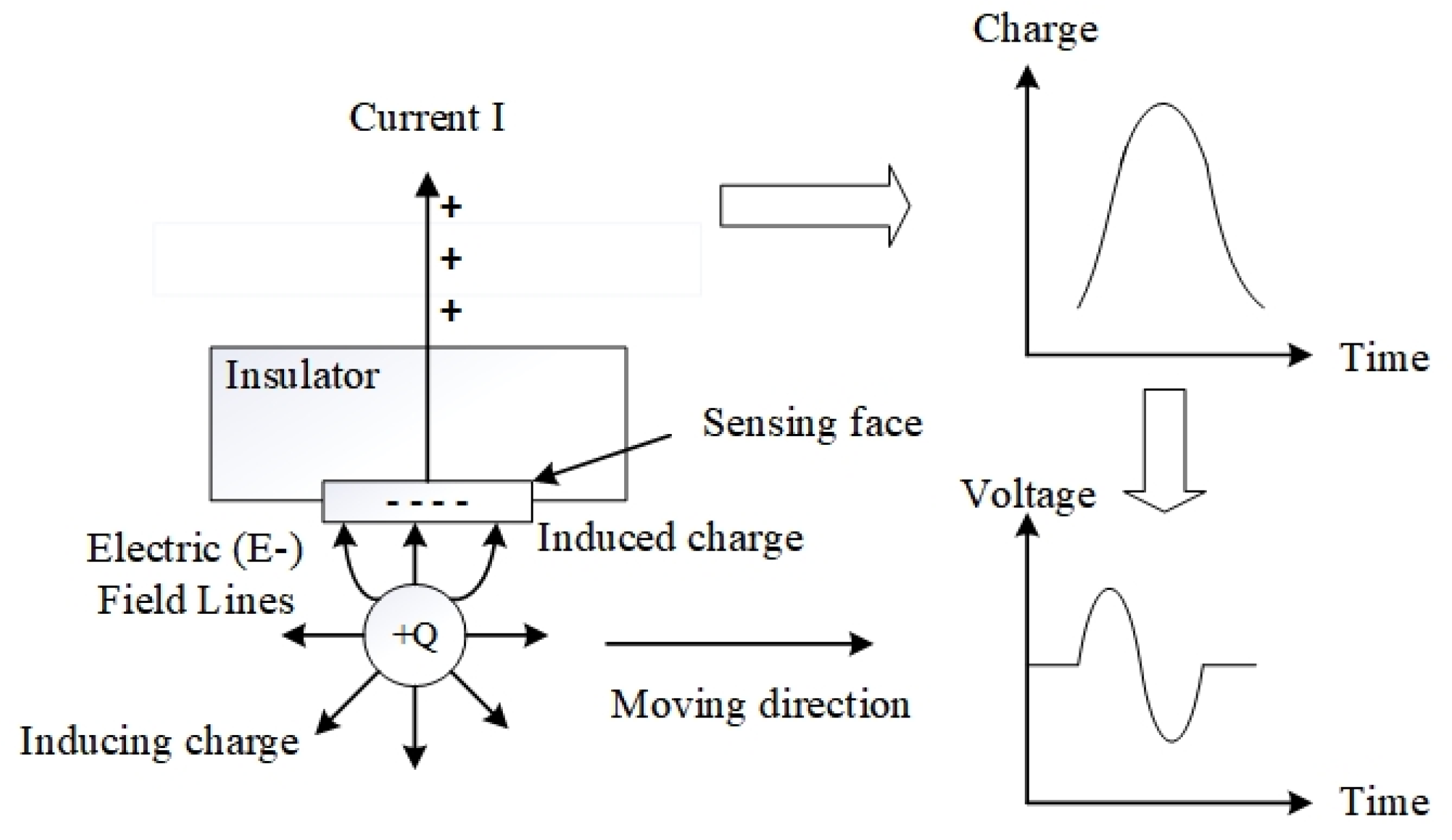
During the operation of mechanical equipment, friction due to the relative movement of the contact surfaces produces a series of physical, chemical, and mechanical changes. Numerous friction and wear phenomena occur in the presence of large amounts of static electricity. Electrostatic monitoring in a mechanical system is used to monitor the static charge in the friction and wear regions, as well as to judge the current operating state of the system along with the performance degradation trend with respect to the monitoring signal. In this study, electrostatic oil-line sensors (OLS) based on the principle of electrostatic electricity have been simulated to explore the regularity of change.
Sensor technology has found widespread applications in diverse fields, and researchers have carried out substantial and productive studies utilizing sensors. Yan et al. [
1]. constructed the CDTFAFN, an innovative multi-sensor data fusion model, and established a dedicated intelligent mechanical fault diagnosis framework based on this model. Ahuja, P. et al. [
2] made significant advances in the study of therapeutic drug glycosylation by employing electrochemical biosensors. Wang et al. [
3] used a grating sensor to measure blood pressure and heart rate, obtaining pulse waveforms equivalent to vascular pulsations. In real life, electrostatic sensors are primarily used in various applications such as pneumatic solid flow measurement, measurement of particulate emissions, fluidized bed monitoring, online particle size measurement, burner flame monitoring, measurement of mechanical system speed and radial vibration, monitoring of conveyor belt, mechanical wear, and human activity, etc. Electrostatic sensors mainly monitor the aero-engine states and bearing wear sites when used in the mechanical wear states [
4]. Zhang [
5] and Qian et al. [
6] used multiple electrode arrays to study the characteristics of gas–solid two-phase flow in a square pipe and measured the cross-sectional velocity and concentration distribution of particles under thin conditions of different wind speeds and particle mass flow rates. Both authors adopted mathematical models that were rather complicated. Zhang and Feng et al. [
7,
8] used electrostatic sensors to study the aero-engine gas path. The difference between the works of Zhang and Feng was that Zhang made sensors and designed circuits to eliminate noise and interference in electrostatic signals, while Feng optimally designed sensors according to their characteristic parameters. Zhong et al. [
9] used electrostatic sensors to obtain accurate information about charged particles, such as the particle centroid and particle space position. Ali et al. [
10] used electrostatic sensors based on multi-physical field coupling to study particle motion trajectories and complex gas path geometries. These studies have demonstrated the use of electrostatic sensors in various applications.
The above researchers used electrostatic sensors to study different aspects. Several authors have used different shapes of electrostatic sensors in their research. Liu [
11,
12] presented a three-dimensional (3D) model of two sensors for electrostatic monitoring. Mao [
13] proposed and tested the mathematical model of an OLS using a test bed. Heydarianasl [
14] established mathematical models and theoretically analyzed various shapes of electrostatic sensors, such as rings, quarter rings, and rectangles. Yu [
15] developed a 3D finite element model to analyze the coupled interactions of electrostatic forces, fluid–solid dynamics, and multiple entanglements in a comb resonance electrostatic sensor. Heydarianasl and Hu et al. [
16,
17] used particle swarm optimization and preamplifier optimization methods, respectively, to optimize electrostatic sensors with different shapes, which improved the overall sensitivity of the sensors. Most of the above studies on electrostatic sensors were based on mathematical models; the use of 3D simulation software was limited, and research on the performance parameters of the sensor itself was not comprehensive. So, more and more people are now choosing to solve problems with finite elements. Wang et al. [
18] simulated the process of fatigue crack extension by using a combination of methods with finite elements. Solhmirzaei et al. [
19] used the finite element method to test the beams. Currently, most of the studies on OLS mainly focus on the quantity, shape and its applications, while the exploration of its intrinsic properties is still relatively insufficient. For this reason, this paper adopts the finite element modeling simulation method to analyze the sensitivity and efficiency characteristics of OLS in depth in order to fill this research gap.
In this study, the process of charge sensing by OLS is modeled by imposing boundary condition constraints, creating a simulation environment, and applying a charge excitation lee. The change in sensor sensitivity is observed by varying the position of the point charge and the diameter, length, and H/D ratio of the probe. In real life, the charges generated by faulty components are not only point charges, so the study of sensitivity distribution under multiple charges is also necessary. Finally, by comparing the distribution of sensitivity in the axial radial direction between the mathematical model and the simulation model for the same diameter and length of the probe, the correctness of the simulation model can be determined. The correct modeling simulation in this paper reduces the complexity of the mathematical model and describes, in detail, issues such as the effect of the charge position on the sensor parameters. This provides a reference for subsequent studies of multi-sensor and other dynamic sensor characteristics.
3. Model Simulation
To express the spatial distribution of the OLS sensing interval more clearly, two performance parameters—spatial sensitivity and sensor efficiency characteristics—have been introduced. The finite element model is used to simulate and analyze the two performance parameters at different axial and radial positions. A comparison is made between the finite element modeling and the mathematical model for both point and multiple charges, leading to more rigorous simulations.
3.1. Space Sensitivity Simulation Analysis
Based on the principle of electrostatics, the generated electrostatic field varies depending on the position of point charge within the pipe, leading to changes in the amount of charge induced by the electrostatic sensor. To clearly illustrate how the induced charge in the OLS varies with the spatial position of the point charge, spatial sensitivity is introduced as a performance parameter. The theoretical formula is as follows:
where
s is the spatial sensitivity;
q is the charge carried by the point charge; and
Q is the charge that can be induced by the point charge.
In this study, the spatial sensitivity characteristics of OLS mainly focus on the following two aspects: (1) keeping the probe size unchanged and observing the spatial sensitivity distribution by varying the position of the induced charge; (2) analyzing the spatial sensitivity distribution of the induced charge at the same radial position within the pipe while varying the probe size.
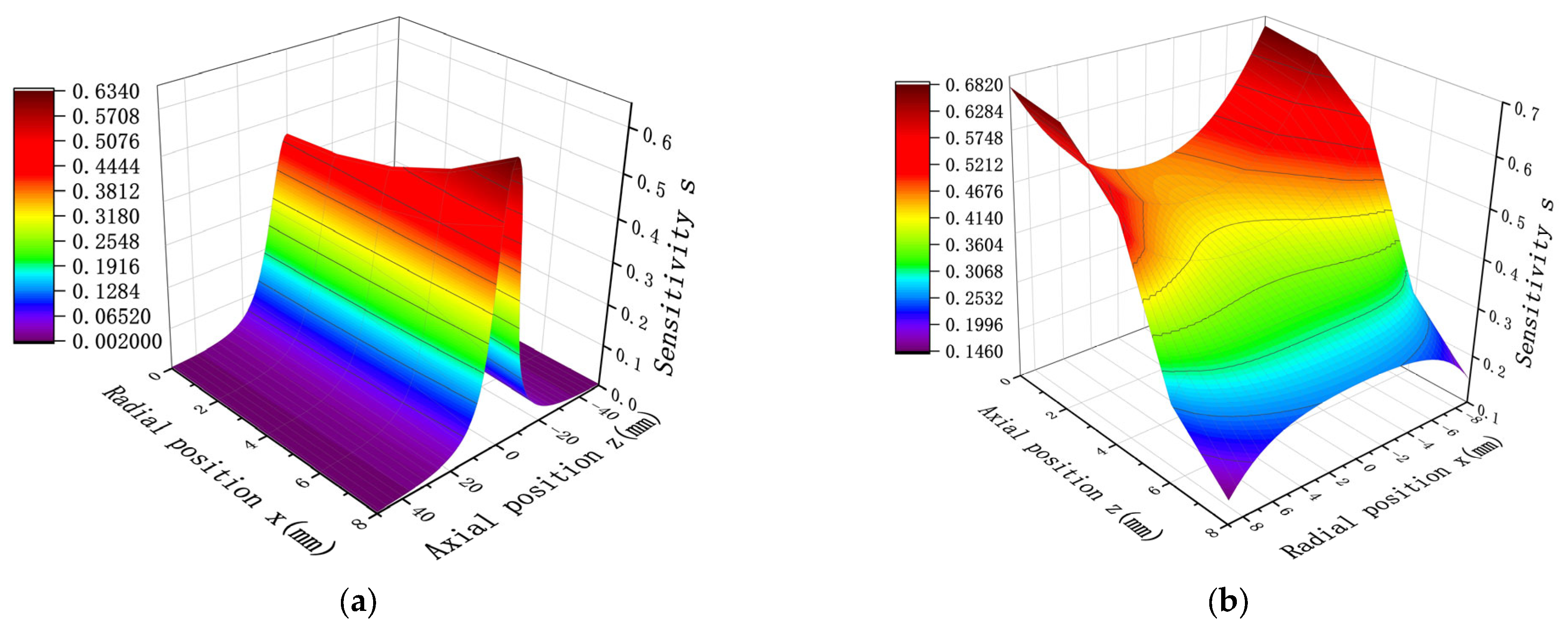
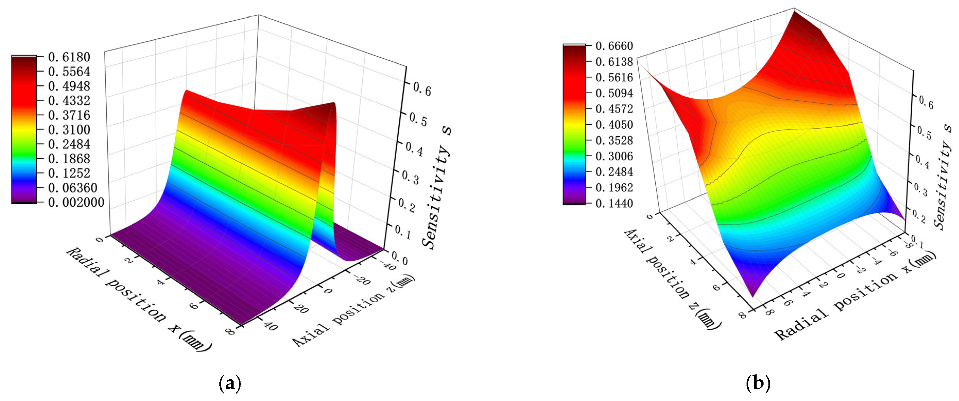
A probe diameter D = 20 mm and length H = 10 mm were set as the initial values, and the sensitivity of the point charge in the sensor at different positions was simulated.
Figure 4 presents the findings for this particular distribution. As illustrated in
Figure 4a, the radial location is fixed, the sensitivity increases as
decreases, and the sensitivity reaches a maximum at z = 0; i.e., the sensitivity is maximum when the point charge is located on the center of the cross-section of the probe. As shown in
Figure 4b, the axial position is fixed. When
< 5; i.e., when the point charge is located inside the probe, the sensitivity decreases with a decrease in
. As the point charge approaches the central axis of the probe, the sensitivity decreases and reaches a minimum at the central axis x = 0. Furthermore, when
> 5; i.e., when the point charge is located outside the probe, the sensitivity increases with a decrease in
. Therefore, the shorter the distance of the point charge from the central axis of the probe, the greater the sensitivity, and the maximum is reached at the central axis x = 0.
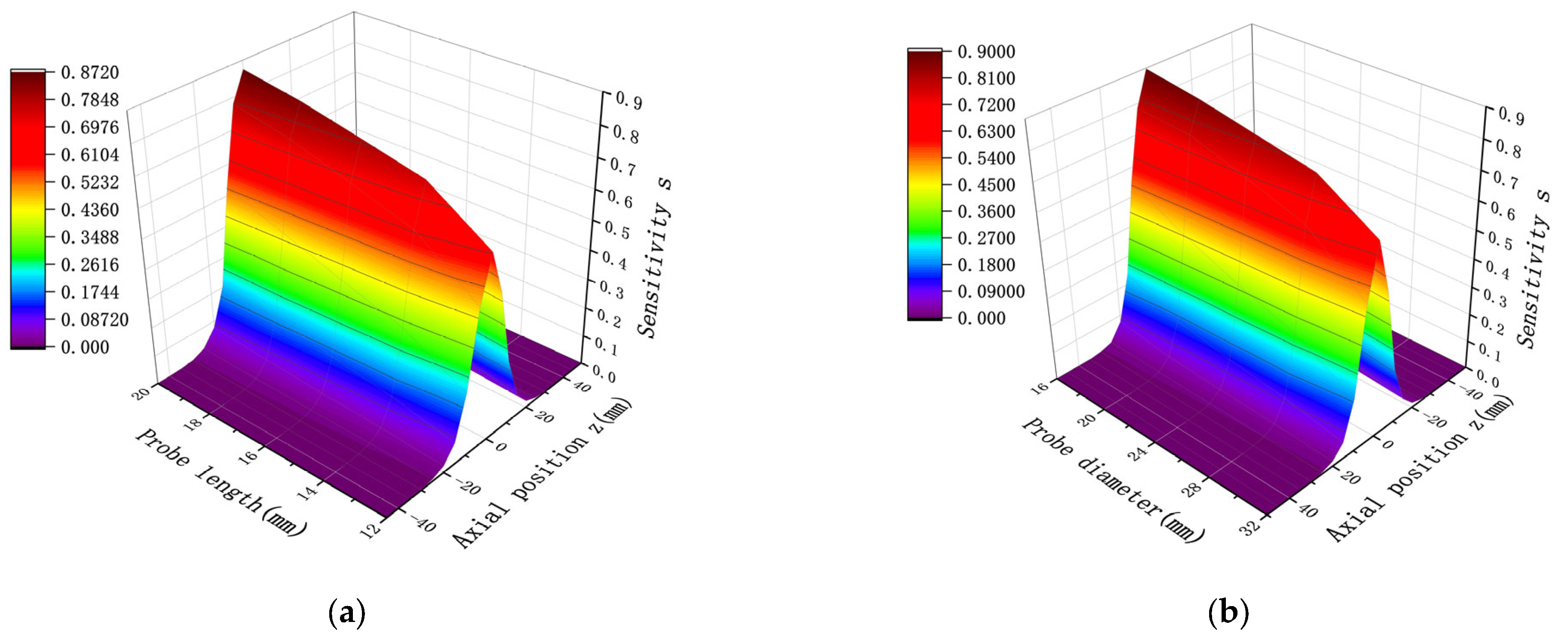
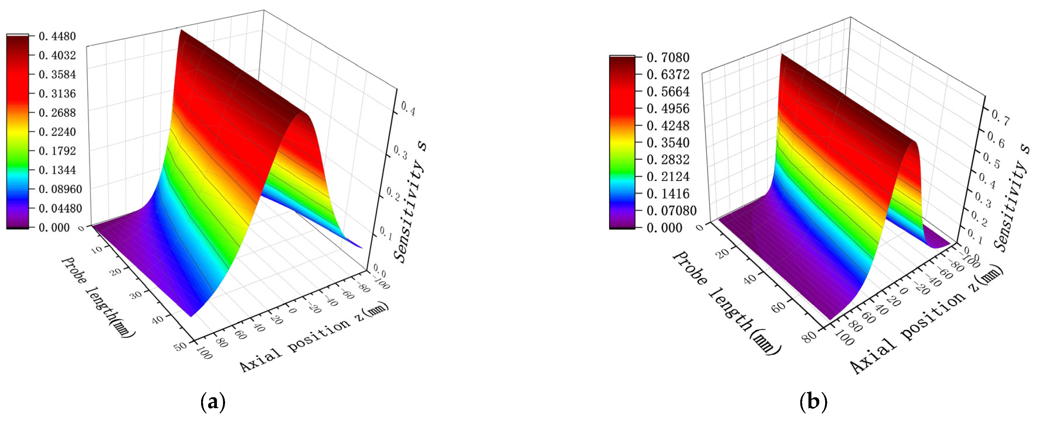
The study of spatial sensitivity with respect to changes in probe size primarily aims to observe the effect of varying one parameter of spatial sensitivity while keeping either the probe length or the diameter fixed. The sensor probe length and diameter were fixed, and a spatial sensitivity simulation curve was obtained for a point charge located at the same radial location, with x = 0. The distribution results are shown in
Figure 5. As demonstrated in
Figure 5a, when the radial position is fixed, an increase in the probe length of the sensor results in higher sensitivity, following an overall trend of increasing sensitivity with length. Additionally for sensors with the same probe length, sensitivity increases as the position approaches x = 0. Therefore, when the probe diameter is fixed, increasing the probe length is an effective way to enhance sensitivity. As evident in
Figure 5b, the sensitivity distribution can be divided into two regions. When the point charge is located outside the corresponding length of the probe, an increase in diameter leads to higher sensitivity. However, when the point charge is within the corresponding length of the probe, an increase in diameter reduces the sensitivity. Since sensor research primarily focuses on improving sensitivity within the inner region of the probe, reducing the sensor diameter while keeping the probe length fixed is also an effective approach to enhance sensitivity.
3.2. Comparative Analysis of Finite Element and Mathematical Model
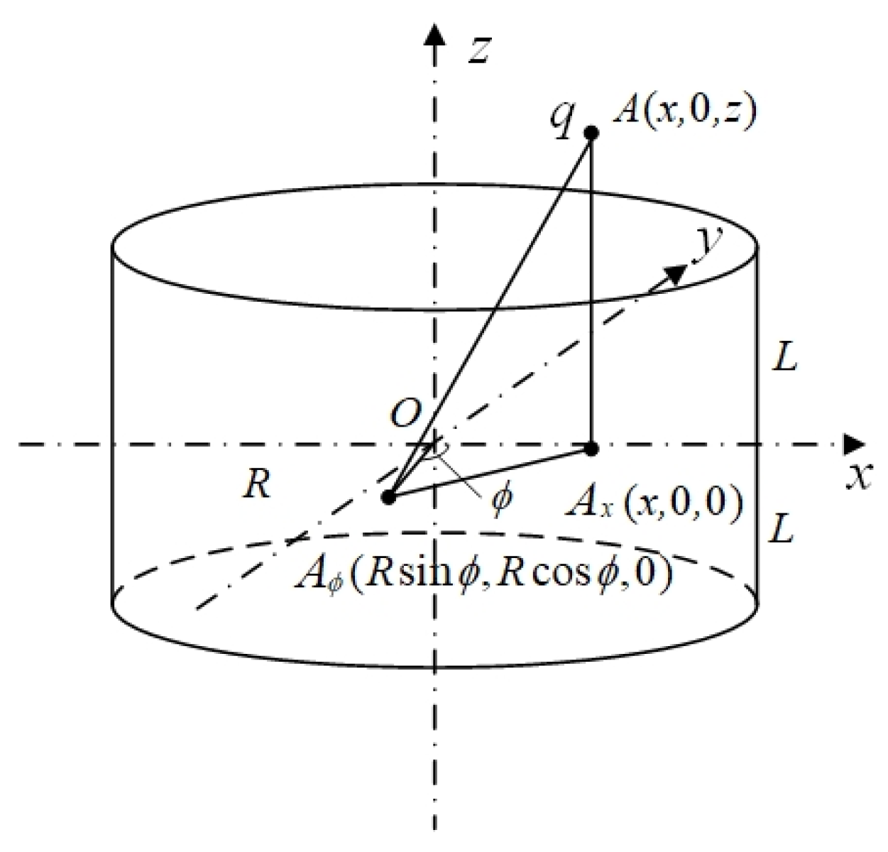
In this paper, we will use the method of comparing with the mathematical model to verify the correctness of the constructed finite element simulation model in order to increase the credibility of the model. In the mathematical model, to obtain the charge Q induced by the ring probe, establishing a theoretical model with the center O of the ring probe as the origin, the axis of the probe as the
z-axis, and the middle cross-section of the probe as the xOy plane is necessary, as shown in
Figure 6.
The probe has a length of 2 L and a diameter of 2 R. Suppose a point charge q is located at point A (x,0,z) inside the probe. The projection of point A onto the plane is denoted as
, where x represents the radial position of the point charge within the probe, and z represents the axial position of the point charge within the probe. At this point, the induced charge Q on the probe is given by the following:
where
is the angle between the probe on the plane and the line between
and the coordinate origin and O
.
In order to verify the reasonableness of the simulation model, space sensitivity is selected as the research parameter in this study, and with the typical dimensions of the electrode diameter and height set to D = 20 mm and H = 10 mm, respectively, the induced charge of the probe electrode at different radial and axial positions is calculated by establishing a mathematical model, and the results are compared and analyzed with the simulation data shown in
Figure 4. Under the above conditions, the mathematical modeling calculations obtained are shown in
Figure 7.
By comparing the results of
Figure 4 with those of
Figure 7, it can be found that under the same values of D and H, the mathematical model calculation results of spatial sensitivity show distribution trend that is a highly consistent with the simulation results. Specifically, when the radial position is fixed, the sensitivity achieves the maximum value at z = 0. When the axial position is fixed, in the range of
< 5 mm, the sensitivity decreases with the decrease in
; while in the region of
> 5 mm, the sensitivity increases with the decrease in
. After quantitative analysis, the relative deviation rates (based on the average value) between the mathematical model and the simulation model in the radial and axial directions are 2.71% and 2.36%, respectively.
In the following, we choose the same diameter and length conditions as in
Figure 5, resulting in the mathematical calculations shown in
Figure 8.
Comparison of the results in
Figure 5 and
Figure 8 shows that the results of the distribution trend of spatial sensitivity remain the same for the same D and H. Specifically, as the sensor probe length H increases and the probe diameter D decreases, the spatial sensitivity increases, and the sensitivity still takes the maximum value at Z = 0. After quantitative analysis, the relative deviation rates (based on average values) between the mathematical model and the simulation model for length and diameter are 2.52% and 2.67%, respectively. This study establishes a validated simulation model for predictive fault monitoring in rotating machinery systems. This small deviation range fully verifies the accuracy and reliability of the established mathematical model. There may be two reasons for the relative deviation rate between the mathematical model and the simulation model: first, the mathematical model only considers the positional reason when calculating, while the modeling needs to consider the material and other issues; second, when the distance between the charged particles and the induction surface of the detector pole is closer, the center area of the sensor has higher sensitivity to the monitoring of the particles, has the ability to capture the particles near the center, and attracts the electric field lines more strongly, so the simulation results will be slightly higher than the mathematical calculation results. This reduces the number of assumptions required, as well as the cumbersome formulas and steps involved in mathematical calculations, providing a more convenient way of calculating.
3.3. Sensor Efficiency Simulation Analysis
Sensor efficiency is divided into theoretical and working efficiencies. The theoretical efficiency can be obtained through simulation calculations, whereas the working efficiency must be obtained experimentally. Therefore, this study focuses on analyzing the theoretical efficiency based on the simulation results. The theoretical efficiency is expressed as follows:
where
is the theoretical efficiency of the sensor; and
is the amount of electricity induced by the probe when the point charge is at C.
The theoretical efficiency of the sensor calculated using Equation (5) can also be considered as the spatial sensitivity at the particular location.
According to the spatial sensitivity distribution law caused by changes in the probe size, discussed in
Section 3.1., an important parameter influencing the spatial sensitivity of the probe is the length-to-diameter ratio. To achieve higher sensitivity, this ratio must be increased. Therefore, to analyze the theoretical efficiency of the sensor more directly, we assess efficiency based on the value of
.
where
is length-to-diameter ratio;
H is the length of the probe; and
D is the diameter of the probe.
Since measuring points within the sensor probe area are diverse and can be distributed anywhere, fixing the measuring points is necessary to study the relationship between and sensor efficiency. Considering the above analysis of the spatial sensitivity of the sensor, the sensitivity change at the center of the sensor probe (Point O) is the most significant. Therefore, point O can be used as a reference point to evaluate the efficiency of the sensor.
is fixed and the probe length is changed to observe the sensitivity distribution of the sensor along the axis. The sensitivity distribution for
= 0.5 and
= 1 is presented in
Figure 9. Clearly, when
is fixed, regardless of changes in probe length, the sensitivity at point O on the central axis remains constant and clustered at a single value. However, when the
value changes, the sensitivity at point O also changes, indicating a variation in sensor efficiency. The same conclusion holds when
is fixed and the probe diameter is varied.
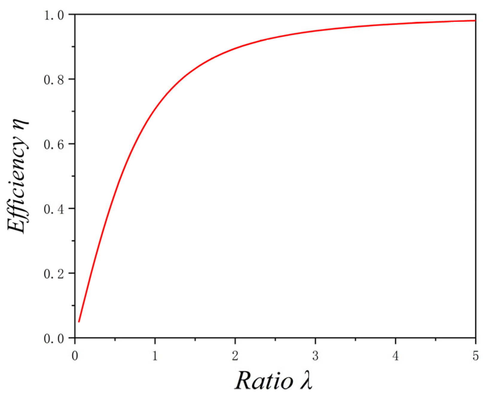
To verify the law, the simulated sensitivity variation trend (variation of the theoretical efficiency of the sensor) under different values of
is shown in
Figure 10. As illustrated in
Figure 10, the sensor efficiency increases as
increases. However, the efficiency rises rapidly at first, and when
reaches 3, the increase begins to level off. Additionally, the theoretical efficiency remains consistently below 1.
3.4. Comparative Analysis of Point and Multiple Charges
In reality, when monitoring component failure using an electrostatic sensor, the particles produced in the wear area are not point-charge particles, but rather multiple charge particles, with their number constantly changing. According to the superposition principle of the electrostatic field, when multiple charges exist in the induction region, their electric field strengths can be superimposed at any given point in space. Therefore, the output characteristics of multiple applied charges can be simulated based on the results of a single applied charge simulation.
To better investigate the characteristic parameter distribution of the oil line sensors under multiple charge conditions, the approach outlined in
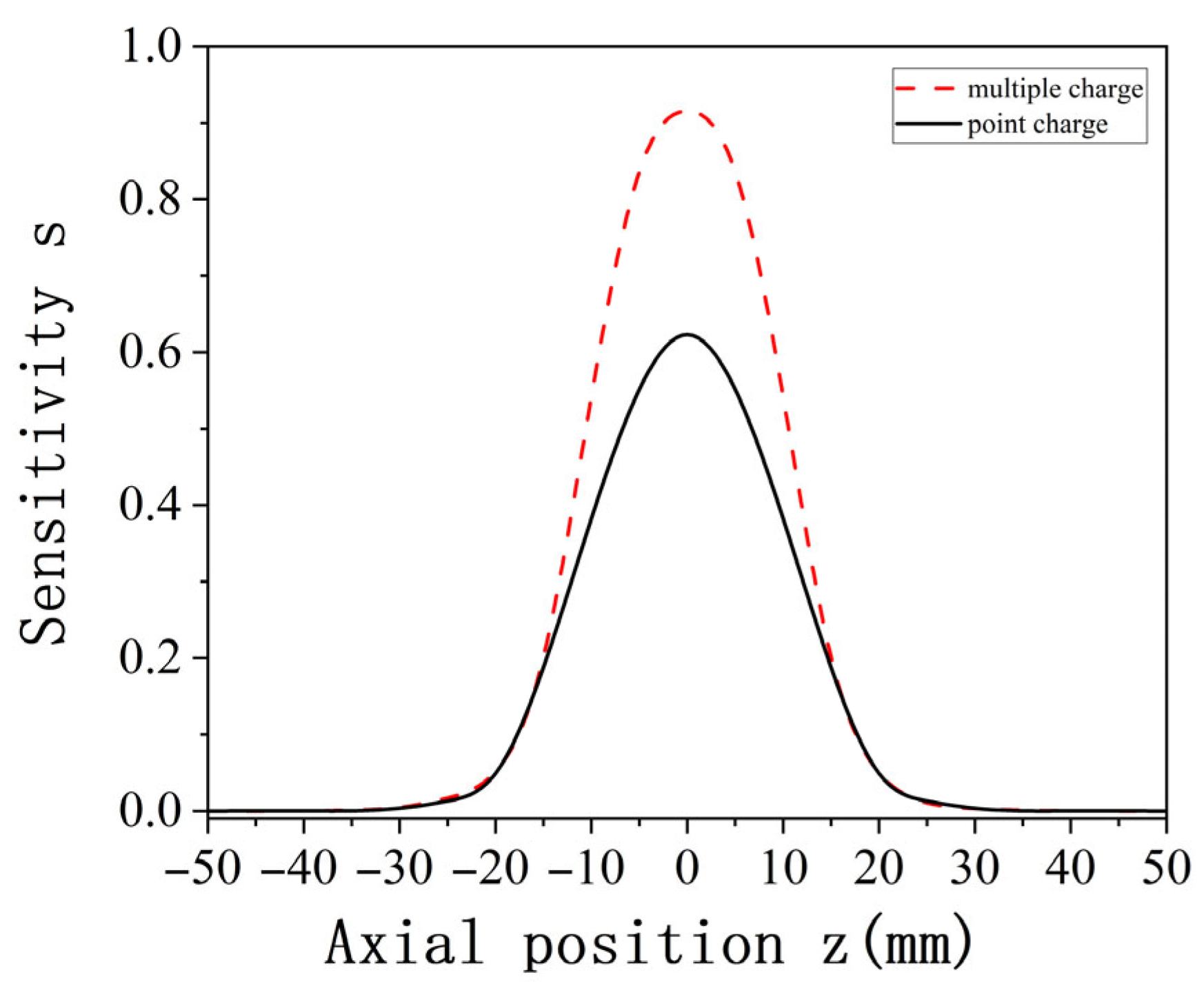
Section 2.2 is adopted. The established model, based on the point charge simulation process, is used to simulate and analyze the spatial sensitivity of multiple charges. The simulation results for both point charge and multiple charge spatial sensitivity are shown in
Figure 11.
Figure 11 demonstrates that the spatial sensitivity distribution trend under multiple charges is consistent with that for a point charge. When the charge is located at the axial position z = 0, corresponding to the central axial section of the pipeline, the sensitivity reaches its maximum. Additionally, the sensitivity distribution on both sides of the radial position z = 0 is symmetric.
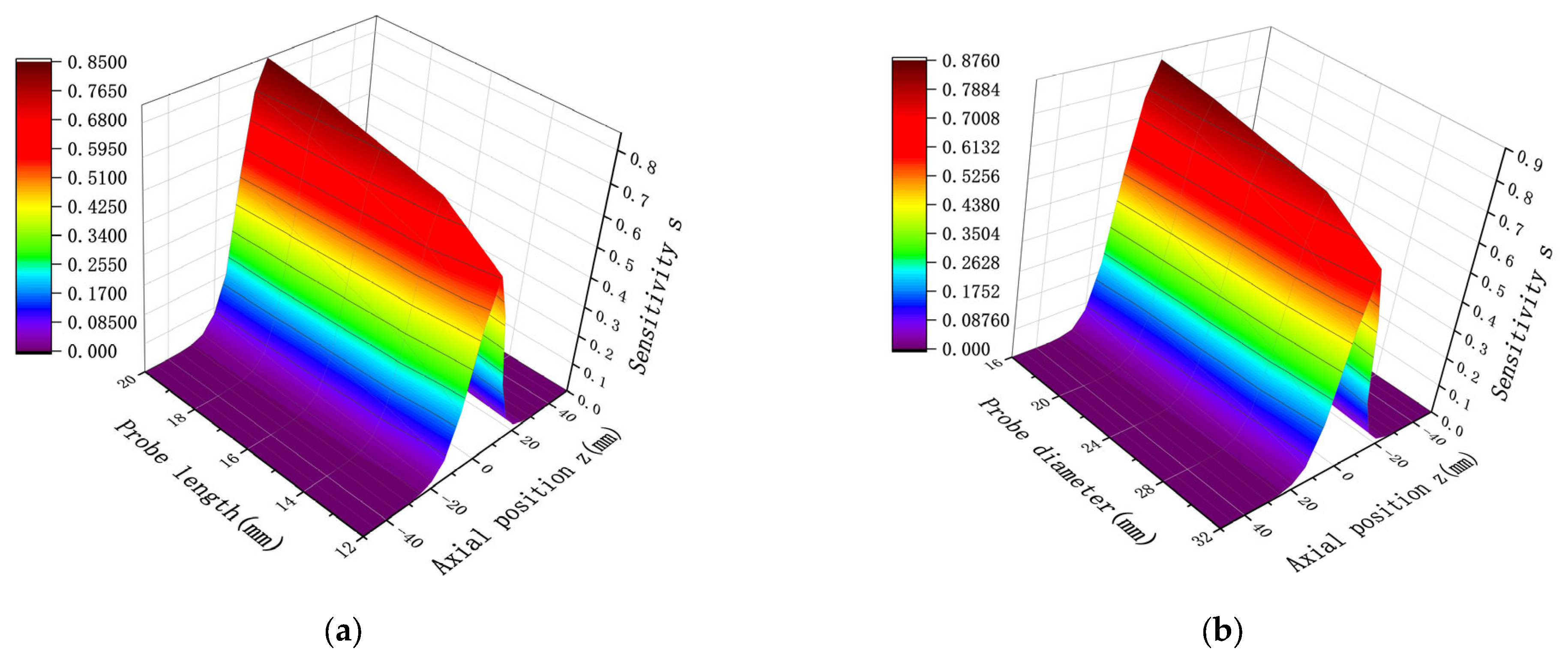
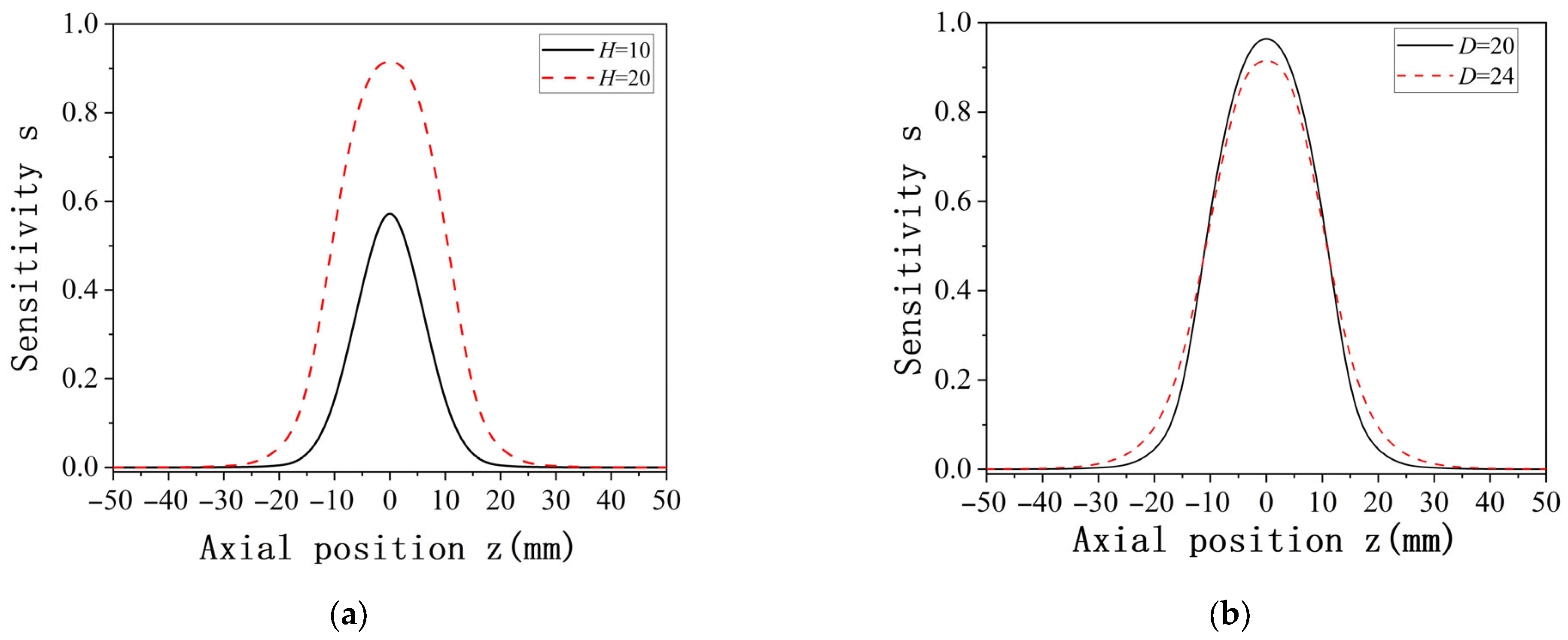
The spatial sensitivity under multiple charges also varies with changes in the length and width of the probe. When the probe diameter is fixed while the length is varied, and when the length is fixed while the diameter is varied, the resulting spatial sensitivity distribution under multiple charges is shown in
Figure 12. As is evident in
Figure 12, despite differences in probe length H and diameter D, the overall sensitivity distribution trend remains unchanged. This trend is consistent with the sensitivity distribution observed under point charge and follows a normal distribution pattern. The sensitivity distribution is symmetric about the axial position z = 0, where the sensitivity reaches its maximum value. Furthermore, in the presence of multiple charges, the sensor sensitivity is proportional to the length of the probe and inversely proportional to its diameter. Higher sensitivity is achieved when the length increases and the diameter decreases. These simulation results confirm that the sensitivity distribution characteristics for multiple charges can be effectively derived from point charge simulation analysis.


