

Superconducting Quantum Magnetometers for Brain Investigations


Abstract
1. Introduction
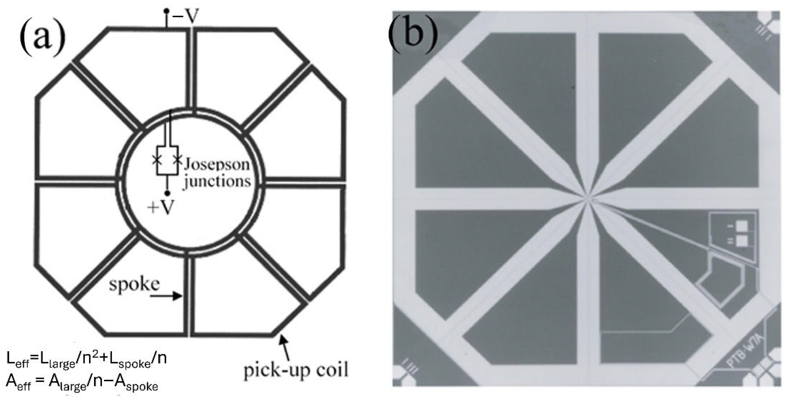
2. SQUIDs
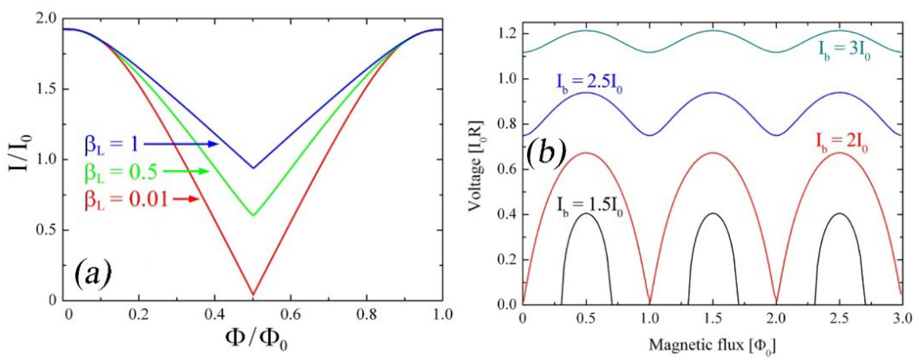
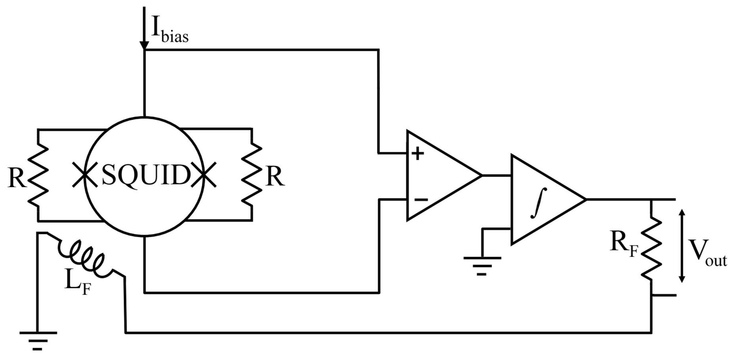
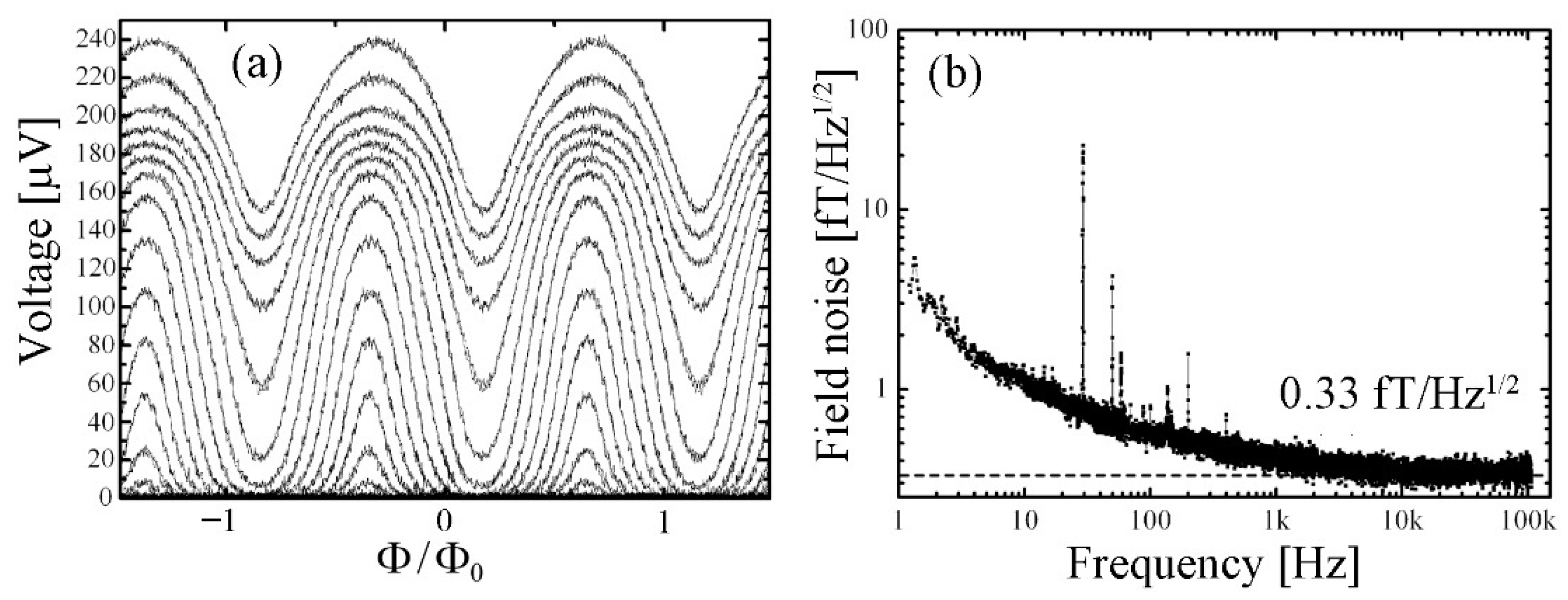
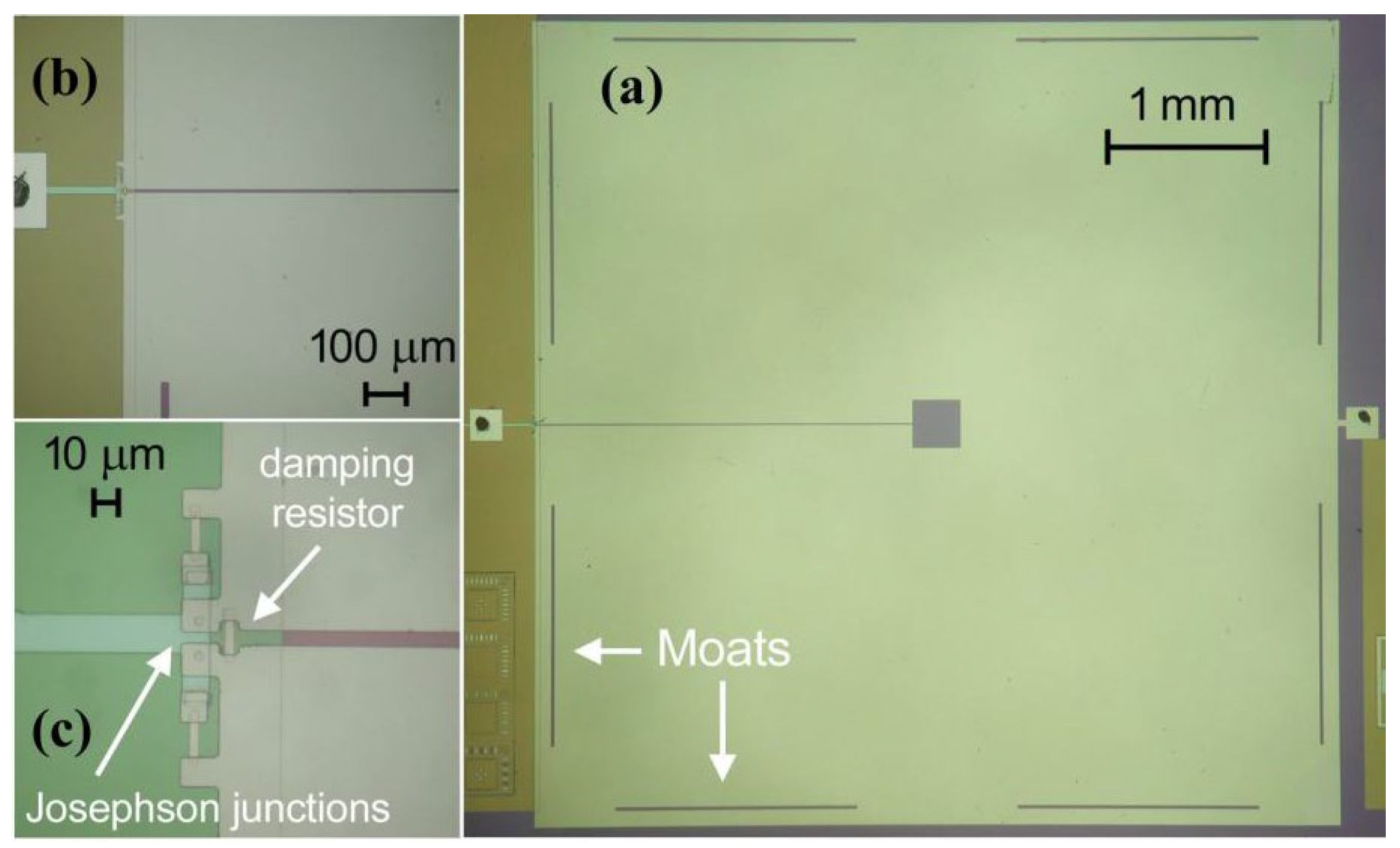
2.1. Working Principles
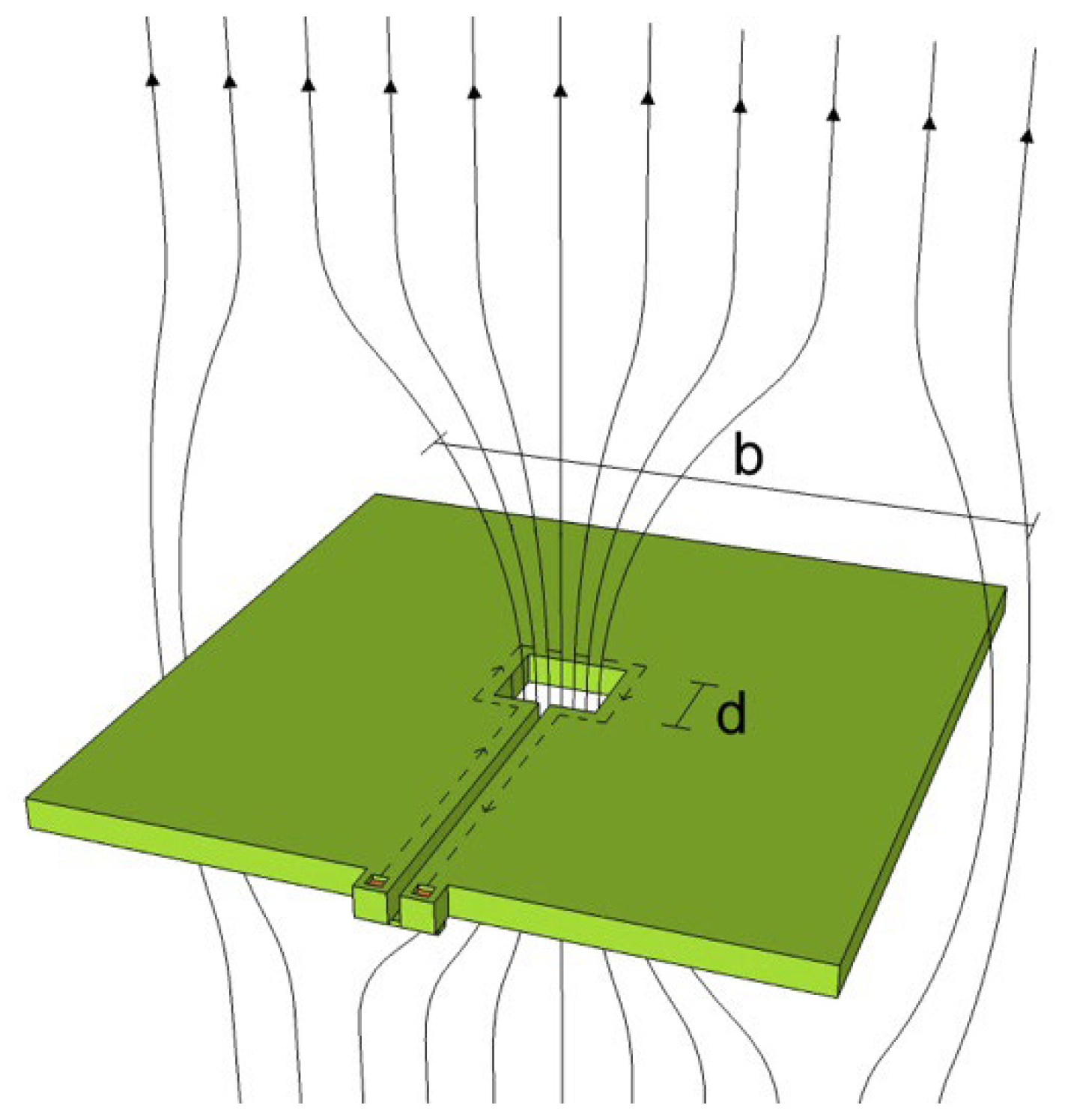
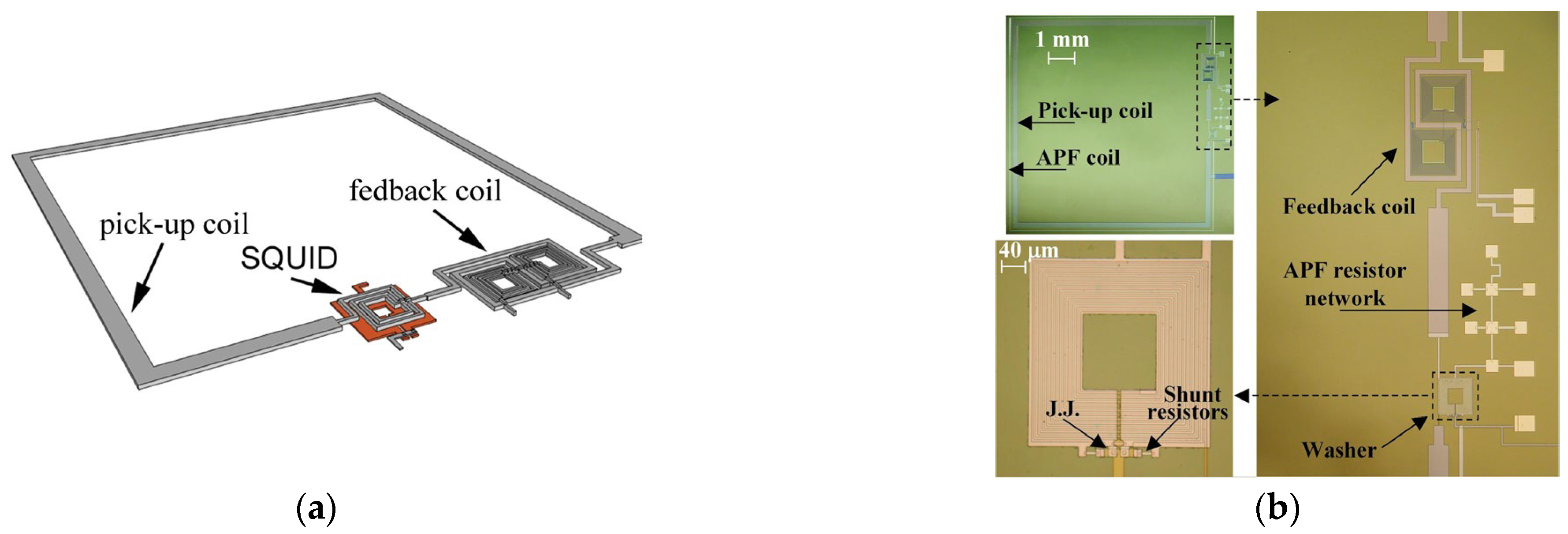
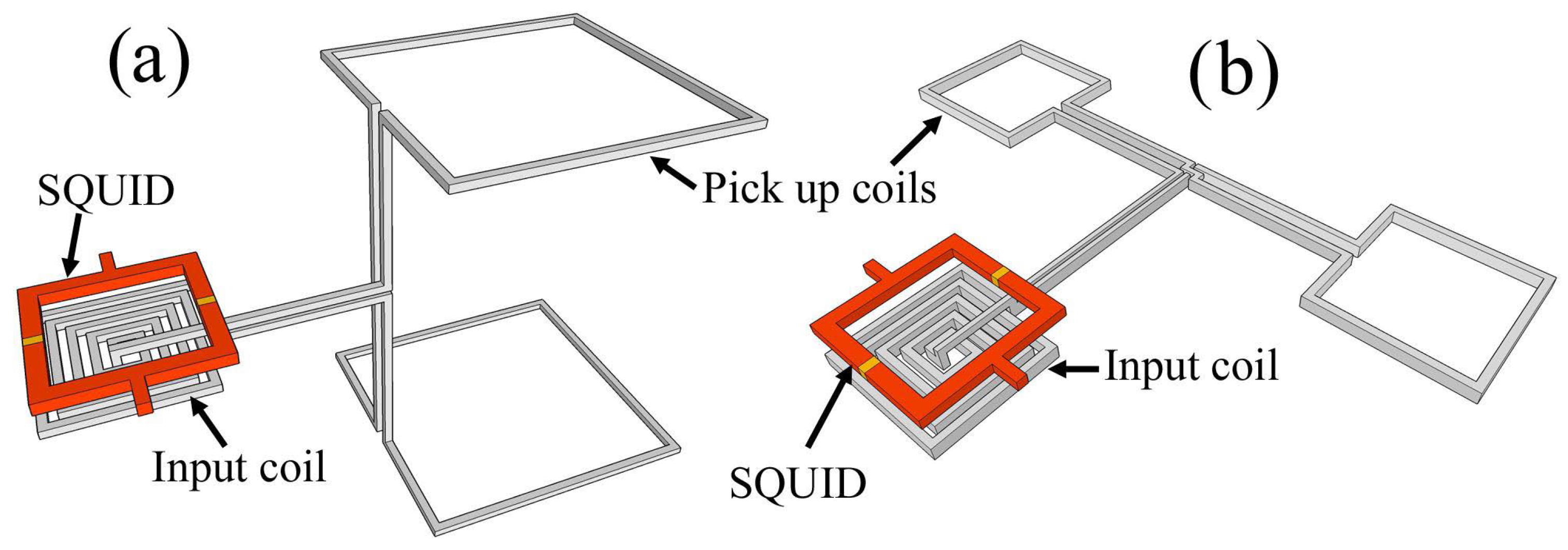
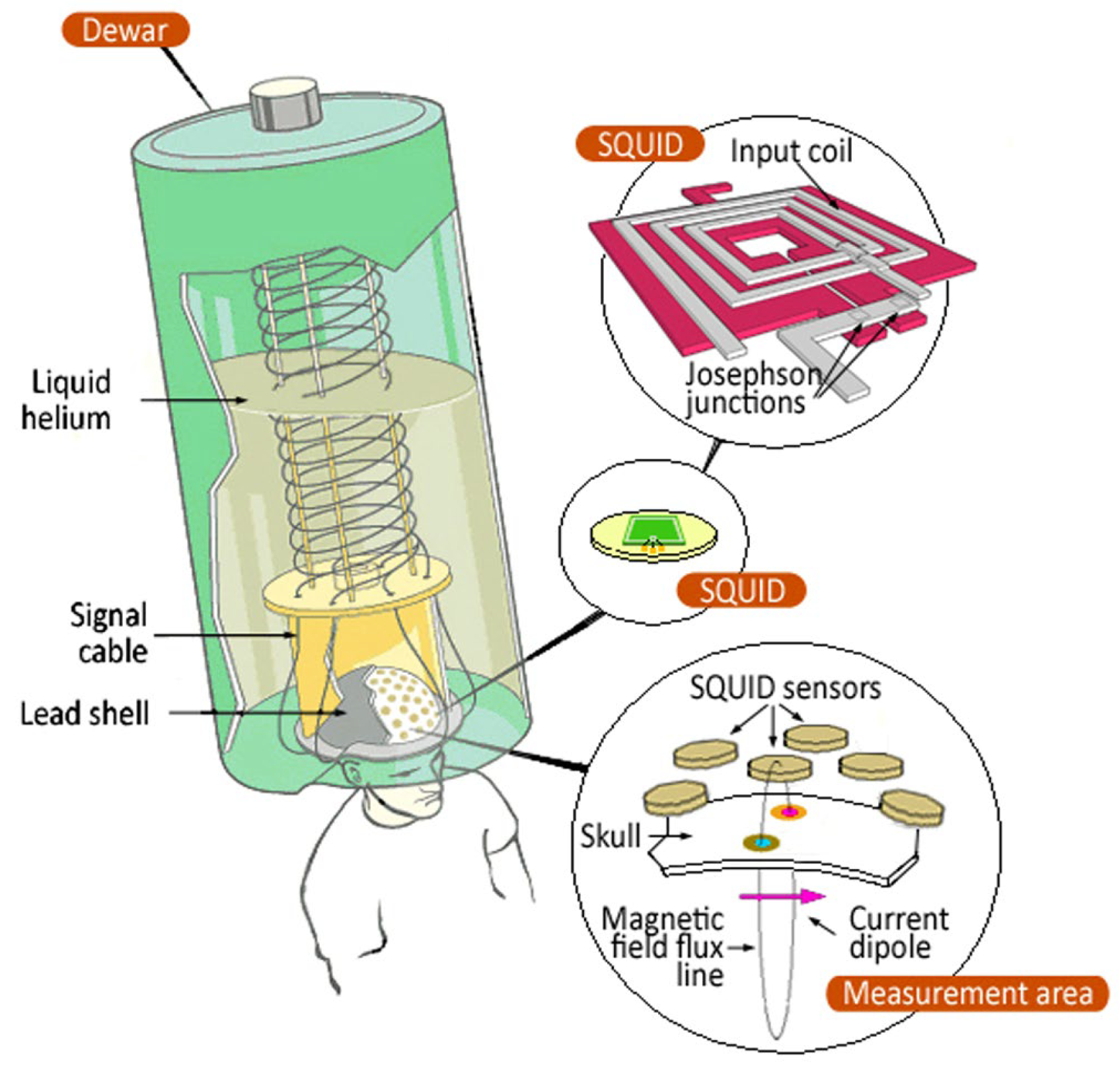
2.2. Superconducting Magnetometer and Gradiometer Configurations
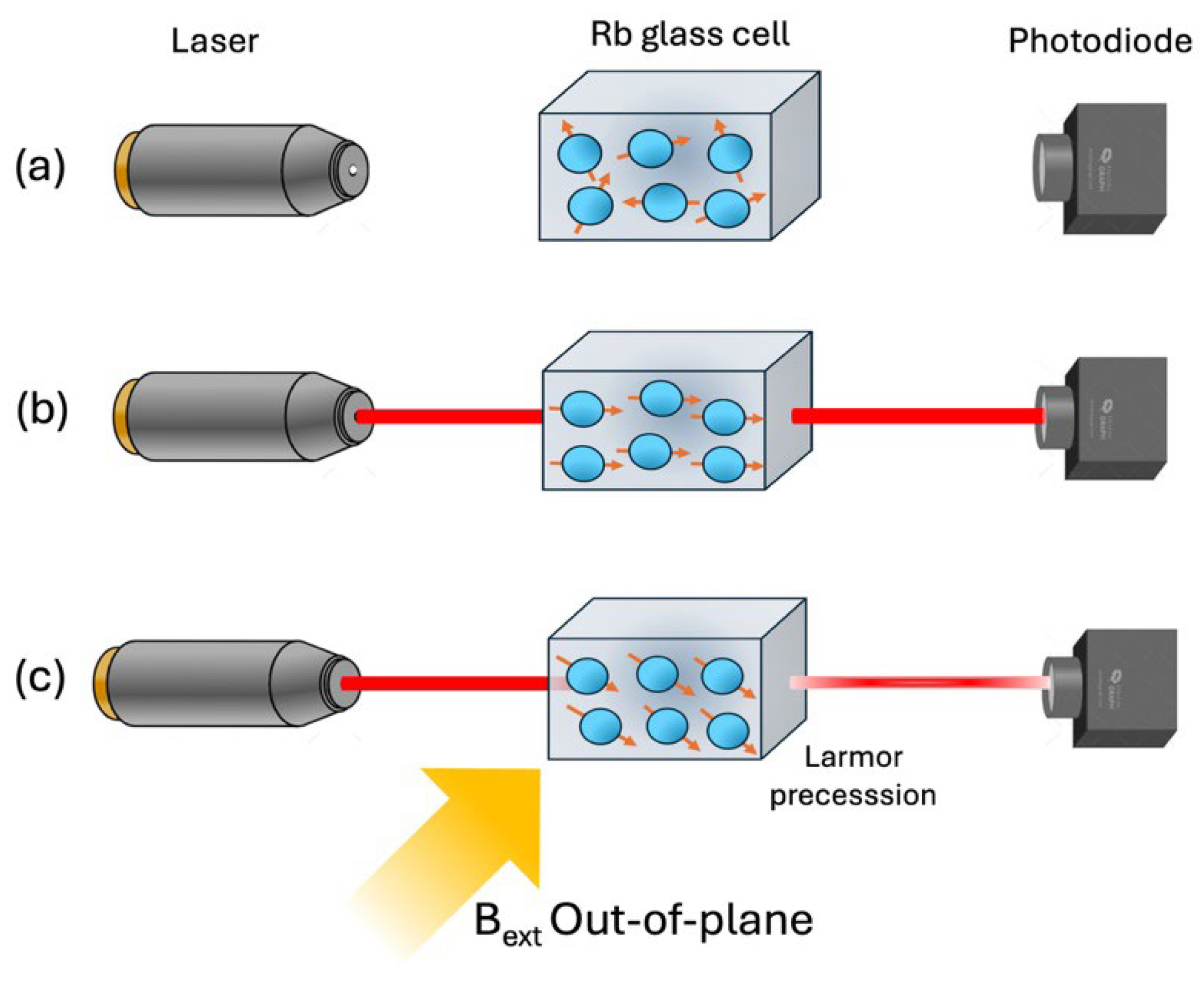
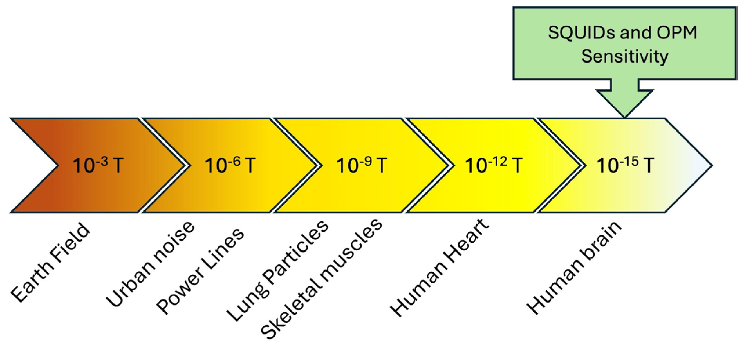
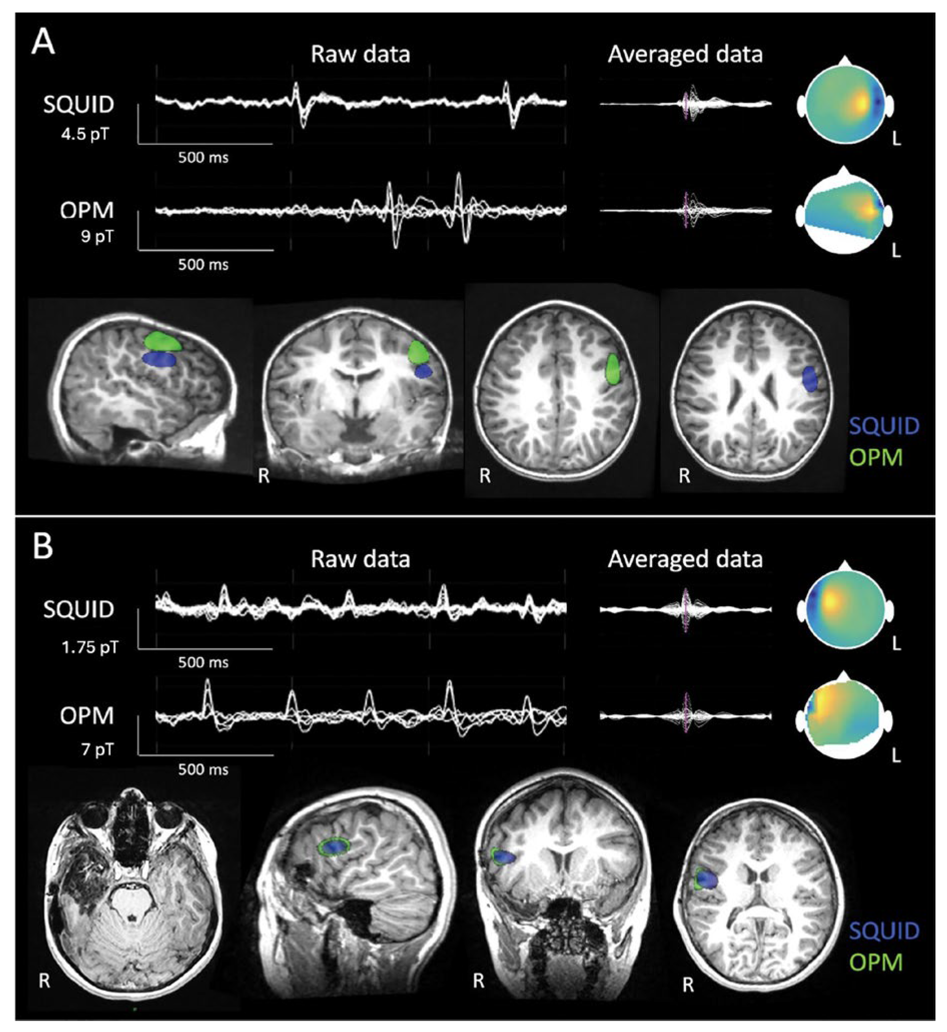
3. SQUID Magnetometer and Optically Pumping Magnetometer (OPM) Comparison
4. Brain Investigation by Magnetoencephalography
4.1. What Is Magnetoencephalography
4.2. MEG Signals
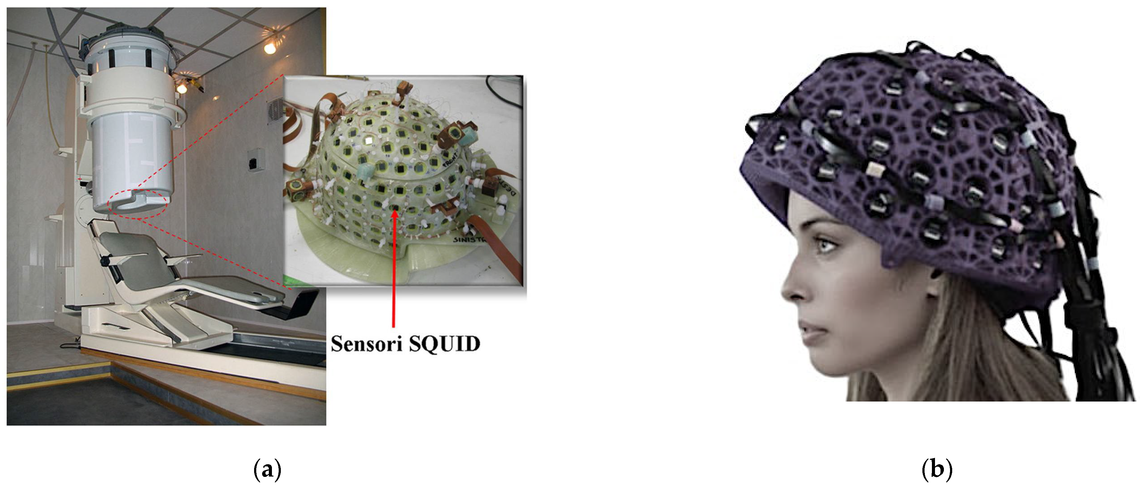
4.3. MEG System Description
5. MEG Clinical Applications
6. Conclusions and Perspectives
Author Contributions
Funding
Acknowledgments
Conflicts of Interest
References
- Cohen, D.; Halgren, E. Magnetoencephalography. In Encyclopedia of Neuroscience; Elsevier: Amsterdam, The Netherlands, 2009; Volume 5, pp. 615–622. [Google Scholar]
- Hämäläinen, M.; Hari, R.; Ilmoniemi, R.; Knuutila, J.; Lounasmaa, O. Magnetoencephalography-theory, instrumentation, and applications to noninvasive studies of the working human brain. Rev. Mod. Phys. 1993, 65, 413–497. [Google Scholar] [CrossRef]
- Del Gratta, C.; Pizzella, V.; Tecchio, F.; Romani, G.-L. Magnetoencephalography—A noninvasive brain imaging method with 1 ms time resolution. Rep. Progr. Phys. 2001, 64, 1759–1814. [Google Scholar] [CrossRef]
- Degen, C.L.; Reinhard, F.; Cappellaro, P. Quantum sensing. Rev. Mod. Phys. 2017, 89, 1. [Google Scholar] [CrossRef]
- Granata, C.; Vettoliere, A. Nano Superconducting Quantum Interference device: A powerful tool for nanoscale investigations. Phys. Rep. 2016, 614, 1. [Google Scholar] [CrossRef]
- Granata, C.; Silvestrini, P.; Vettoliere, A. Nano Superconducting Quantum Interference Device. In 21st Century Nanoscience–A Handbook; CRC Press: Boca Raton, FL, USA, 2020. [Google Scholar]
- Martínez-Pérez, M.J.; Koelle, D. NanoSQUIDs: Basics & recent advances. Phys. Sci. Rev. 2017, 2, 20175001. [Google Scholar] [CrossRef]
- Clarke, J.; Braginski, A.I. The SQUID Handbook Vol I: Fundamentals and Technology of SQUIDs and SQUID Systems; Wiley-VCH Verlag GmbH & Co. KgaA: Weinheim, Germany, 2004. [Google Scholar]
- Seidel, P. Applied Superconductivity: Handbook on Devices and Applications; Wiley: Weinheim, Germany, 2015. [Google Scholar]
- Fagaly, R.K. Superconducting quantum interference device instruments and applications. Rev. Sci. Instrum. 2006, 77, 101101. [Google Scholar] [CrossRef]
- Vettoliere, A.; Silvestrini, P.; Granata, C. Superconducting quantum magnetic sensing. In Quantum Materials, Devices, and Applications; Henini, M., Rodrigues, M.O., Eds.; Elsevier: Amsterdam, The Netherlands, 2023; pp. 43–85. [Google Scholar] [CrossRef]
- Tierney, T.M.; Holmes, N.; Mellor, S.; López, J.D.; Roberts, G.; Hill, R.M.; Boto, E.; Leggett, J.; Shah, V.; Brookes, M.J.; et al. Optically pumped magnetometers: From quantum origins to multi-channel magnetoencephalography. NeuroImage 2019, 199, 598–608. [Google Scholar] [CrossRef]
- Kominis, I.K.; Kornack, T.W.; Allred, J.C.; Romalis, M.V. A subfemtotesla multichannel atomic magnetometer. Nature 2003, 422, 596–599. [Google Scholar] [CrossRef]
- Xie, Y.; Yu, H.; Zhu, Y.; Qin, X.; Rong, X.; Duan, C.-K.; Du, J. A hybrid magnetometer towards femtotesla sensitivity under ambient conditions. Sci. Bull. 2021, 66, 127–132. [Google Scholar] [CrossRef]
- Taylor, J.M.; Cappellaro, M.P.; Childres, L.; Jiang, L.; Budker, D.; Hemmer, P.R.; Yacoby, A.; Walsworth, R.; Lukin, M.D. High-sensitivity diamond magnetometer with nanoscale resolution. Nat. Phys. 2008, 4, 810–816. [Google Scholar] [CrossRef]
- Barone, A.; Paterno, G. Physiccs and Applications of the Josephson Efffect; John Wiley & Sons: Hoboken, NJ, USA, 1982. [Google Scholar]
- Doll, R.; Nabauer, M. Experimental proof of magnetic flux quantizaton in a superconduting ring. Phys. Rev. 1965, 138, A744–A746. [Google Scholar]
- Stewart, W.C. Current-voltage characteristics of Josephson junctions. Appl. Phys. Lett. 1968, 12, 277–280. [Google Scholar] [CrossRef]
- Tesche, C.; Clarke, J. DC SQUID: Noise and optimization. J. Low Temp. Phys. 1977, 29, 301–331. [Google Scholar] [CrossRef]
- Ryhanen, T.; Seppa, H.; Illimoniemi, R.; Knuutila, J. SQUID magnetometers for low-frequency applications. J. Low Temp. Phys. 1989, 76, 287–386. [Google Scholar] [CrossRef]
- McCumber, D.E. Effect of ac impedance on dc voltage-current characteristics of Josephson junctions. J. Appl. Phys. 1968, 39, 3113–3118. [Google Scholar] [CrossRef]
- Voss, R.F.; Laibowitz, R.B.; Broers, A.N.; Raider, S.I.; Knoedler, C.M.; Viggiano, J.M. Ultra low noise Nb DC SQUIDs. IEEE Trans. Magn. 1981, 17, 395–399. [Google Scholar] [CrossRef]
- Cantor, R. DC SQUIDS: Design, optimization and practical applications. In SQUID Sensors: Fundamentals, Fabrication and Applications, Series E: Applied Sciences; Weinstock, H., Ed.; Kluwer Academic Publisher: Dordrecht, The Netherlands, 1996; Volume 329, p. 179. [Google Scholar]
- Ketchen, M.B.; Jaycox, J.M. Ultra-low-noise tunnel junction dc SQUID with a tightly coupled planar input coil. Appl. Phys. Lett. 1982, 40, 736–738. [Google Scholar] [CrossRef]
- Mitchell, M.W.; Palacios Alvarez, S. Colloquium: Quantum Limits to the Energy Resolution of Magnetic Field Sensors. Rev. Mod. Phys. 2020, 92, 021001. [Google Scholar] [CrossRef]
- Koch, R.H.; Clarke, J.; Goubau, W.M.; Martinis, J.M.; Pegrum, C.M.; Van Harlingen, D.J. Flicker (1/f) noise in tunnel junction dc-SQUIDs. J. Low Temp. Phys. 1983, 51, 207–224. [Google Scholar] [CrossRef]
- Clarke, J. SQUID fundamentals. In SQUID Sensors: Fundamentals, Fabrication and Application, Series E: Applied Sciences; Weinstock, H., Ed.; Kluwer Academic Publisher: Dordrecht, The Netherlands, 1996; Volume 329, pp. 1–62. [Google Scholar]
- Dantsker, E.; Tanaka, S.; Nilsson, P.A.; Kleiner, R.; Clarke, J. Reduction of 1/f noise in high-Tc dc superconducting quantum interference devices cooled in an ambient magnetic field. Appl. Phys. Lett. 1996, 69, 4099–4101. [Google Scholar] [CrossRef]
- Dantsker, E.; Tanaka, S.; Clarke, J. High-Tc SQUIDs with slots or holes: Low 1/f noise in ambient magnetic fields. Appl. Phys. Lett. 1997, 70, 2037–2039. [Google Scholar] [CrossRef]
- Hasnat, A. Performance optimization of the nano-sized pick-up loop of a dc-SQUID. Phys. C Supercond. Its Appl. 2001, 583, 1353852. [Google Scholar] [CrossRef]
- Koch, R.H.; Sun, J.Z.; Foglietti, V.; Gallagher, W.J. Flux dam: A method to reduce extra low frequency noise when a superconducting magnetometer is exposed to a magnetic field. Appl. Phys. Lett. 1995, 67, 709–711. [Google Scholar] [CrossRef]
- Forgacs, R.L.; Warnick, A.F. Digital-Analog Magnetometer Utilizing Superconducting Sensor. Rev. Sci. Instrum. 1967, 38, 214–220. [Google Scholar] [CrossRef]
- Drung, D.; Dantsker, E.; Ludwig, F.; Koch, H.; Kleiner, R.; Clarke, J.; Krey, S.; Reimer, D.; David, B.; Doessel, O. Low noise YBa2Cu3O7–x SQUID magnetometers operated with additional positive feedback. Appl. Phys. Lett. 1996, 68, 1856–1858. [Google Scholar] [CrossRef]
- Wellstood, F.; Heiden, C.; Clarke, J. Integrated dc SQUID magnetometer with a high slew rate. Rev. Sci. Instrum. 1984, 55, 952. [Google Scholar] [CrossRef]
- Matsuda, M.; Murayama, Y.; Kiryu, S.; Kasai, N.; Kashiwaya, S.; Koyanagi, M.; Endo, T. Directly-coupled dc SQUID magnetometers made of Bi-Sr-Ca-Cu oxide films. IEEE Trans. Magn. 1991, 27, 3043–3046. [Google Scholar] [CrossRef]
- Koelle, D.; Miklich, A.H.; Ludwig, F.; Dantsker, E.; Nemeth, D.T.; Clarke, J. DC SQUID magnetometers from single layers of YBa2Cu3O7-x. Appl. Phys. Lett. 1993, 63, 2271–2273. [Google Scholar] [CrossRef]
- Martinis, J.M.; Clarke, J. Signal and noise theory for a dc SQUID amplifier. J. Low Temp. Phys. 1965, 61, 227–236. [Google Scholar] [CrossRef]
- Ketchen, M.B. Integrated thin-film dc SQUID sensors. IEEE Trans. Magn. 1987, 23, 1650–1657. [Google Scholar] [CrossRef]
- Zhang, Y.; Qin, X.; Liu, G.; Wang, C.; Li, Q.; Yuan, J.; Liu, W. Enhancing Precision in SQUID Sensors: Analyzing Washer Geometry Dependence at the Microscale. Appl. Sci. 2024, 14, 6212. [Google Scholar] [CrossRef]
- Kugai, H.; Nagaishi, T.; Itozaki, H. YBCO Thin film Flux Transformer with Multiturn Input Coil. In Advances in Superconductivity VIII; Hayakawa, H., Enomoto, Y., Eds.; Springer: Tokyo, Japan, 1996; pp. 1145–1148. [Google Scholar]
- Granata, C.; Vettoliere, A.; Russo, M. Improved superconducting quantum interference device magnetometer for low cross talk operation. Appl. Phys. Lett. 2006, 88, 212506. [Google Scholar] [CrossRef]
- Vettoliere, A.; Granata, C. Superconducting Quantum Magnetometer Based on Flux Focusing Effect for High-Sensitivity Applications. Sensors 2024, 24, 3998. [Google Scholar] [CrossRef] [PubMed]
- Enpuku, K.; Sueoka, K.; Yoshida, K.; Irie, F. Effect of damping resistance on voltage versus flux relation of a dc SQUID with large inductance and critical current. J. Appl. Phys. 1985, 57, 1691–1697. [Google Scholar] [CrossRef]
- Enpuku, K.; Muta, T.; Yoshida, K.; Irie, F. Noise characteristics of a dc SQUID with a resistively shunted inductance. J. Appl. Phys. 1985, 58, 1916–1923. [Google Scholar] [CrossRef]
- Zimmerman, J.E. Josephson effect devices and low-frequency field sensing. J. Appl. Phys. 1971, 42, 4483. [Google Scholar] [CrossRef]
- Drung, D.; Cantor, R.; Peters, M.; Scheer, H.J.; Koch, H. Low-noise high-speed dc superconducting quantum interference device magnetometer with simplified feedback electronics. Appl. Phys. Lett. 1990, 57, 406. [Google Scholar] [CrossRef]
- Drung, D.; Cantor, R.; Peters, M.; Ryhanen, T.; Koch, H. A 37 channel dc SQUID magnetometer system. IEEE Trans. Magn. 1991, 27, 3001. [Google Scholar] [CrossRef]
- Koch, R.H.; Ketchen, M.B.; Gallagher, W.J.; Sandstrom, R.L.; Kleinsasser, A.W.; Gambrel, D.R.; Field, T.H.; Matz, H. Magnetic hysteresis in integrated low-Tc SQUID gradiometers. Appl. Phys. Lett. 1991, 58, 1786. [Google Scholar] [CrossRef]
- Drung, D.; Koch, H. An electronic second-order gradiometer for biomagnetic applications in clinical shielded rooms. IEEE Trans. Appl. Supercond. 1993, 3, 2594. [Google Scholar] [CrossRef]
- Drung, D. Low-frequency noise in low-Tc multiloop magnetometers with additional positive feedback. Appl. Phys. Lett. 1995, 67, 1474. [Google Scholar] [CrossRef]
- Drung, D.; Knappe, S.; Koch, H. Theory for the multiloop dc superconducting quantum interference device magnetometer and experimental verification. J. Appl. Phys. 1995, 77, 4088–4098. [Google Scholar] [CrossRef]
- Schmelz, M.; Stolz, R.; Zakosarenko, V.; Schönau, T.; Anders, S.; Fritzsch, L.; Mück, M.; Meyer, M.; Meyer, H.-G. Sub-fT/Hz1/2 resolution and field-stable SQUID magnetometer based on low parasitic capacitance sub-micrometer cross-type Josephson tunnel junctions. Phys. C Supercond. Its Appl. 2012, 482, 27–32. [Google Scholar] [CrossRef]
- Schmelz, M.; Stolz, R.; Zakosarenko, V.; Schonau, T.; Anders, S.; Fritzsch, L.; Muck, M.; Meyer, H.-G. Field-stable SQUID magnetometer with sub-fT Hz−1/2 resolution based on sub-micrometer cross-type Josephson tunnel junctions. Supercond. Sci. Technol. 2011, 24, 065009. [Google Scholar] [CrossRef]
- Schmelz, M.; Vettoliere, A.; Zakosarenko, V.; De Leo, N.; Fretto, M.; Stolz, R.; Granata, C. 3D nanoSQUID based on tunnel nano-junctions with an energy sensitivity of 1.3 h at 4.2 K. Appl. Phys. Lett. 2017, 111, 032604. [Google Scholar] [CrossRef]
- Vrba, J.; Robinson, S.E. SQUID sensor array configurations for magnetoencephalography applications. Supercond. Sci. Technol. 2002, 15, R51. [Google Scholar] [CrossRef]
- Cantor, R.; Ad Hall, J.; Matlachov, A.N.; Volegov, P.L. First-Order Planar Superconducting Quantum Interference Device Gradiometers with Long Baseline. IEEE Trans. Appl. Supercond. 2007, 17, 672. [Google Scholar] [CrossRef]
- Stolz, R.; Fritzsch, L.; Meyer, H.G. LTS SQUID sensor with a new configuration. Supercond. Sci. Technol. 1999, 12, 806. [Google Scholar] [CrossRef]
- Ketchen, M.B. Design Considerations for DC SQUIDs Fabricated in Deep Sub-Micron Technology. IEEE Trans. Magn. 1991, 27, 2916–2919. [Google Scholar] [CrossRef]
- Granata, C.; Vettoliere, A.; Rombetto, S.; Nappi, C.; Russo, M. Performances of compact integrated superconducting magnetometers for biomagnetic imaging. J. Appl. Phys. 2008, 104, 073905. [Google Scholar] [CrossRef]
- Granata, C.; Vettoliere, A.; Nappi, C.; Lisitskiy, M.; Russo, M. Long baseline planar superconducting gradiometer for biomagnetic imaging. Appl. Phys. Lett. 2009, 95, 042502. [Google Scholar] [CrossRef]
- Kang, C.S.; Lee, Y.H.; Kim, K.; Yu, K.K.; Kim, J.M.; Kwon, H.; Kim, I.S.; Park, Y.K.; Lim, H.K.; Lee, S.G. Comparison of magnetocardiograms measured using different SQUID pickup coil configuration. IEEE Trans. Appl. Supercond. 2007, 17, 835. [Google Scholar] [CrossRef]
- Available online: https://starcryo.com/ (accessed on 10 July 2025).
- Available online: http://www.magnicon.com/ (accessed on 10 July 2025).
- Available online: http://www.supracon.com/en/home.html/ (accessed on 10 July 2025).
- Pannetier, M.; Fermon, C.; Le Goff, G.; Simola, J.; Kerr, E. Femtotesla Magnetic Field Measurement with Magnetoresistive Sensors. Science 2004, 304, 1648–1650. [Google Scholar] [CrossRef] [PubMed]
- Luomahaara, J.; Vesterinen, V.; Gronberg, L.; Hassel, J. Kinetic inductance magnetometer. Nat. Commun. 2014, 5, 4872. [Google Scholar] [CrossRef] [PubMed]
- Granata, C.; Vettoliere, A.; Monaco, R. Noise performance of superconductive magnetometers based on long Josephson tunnel junctions. Supercond. Sci. Technol. 2014, 27, 095003. [Google Scholar] [CrossRef]
- Shah, V.; Knappe, S.; Schwindt, P.D.D.; Kitching, J. Subpicotesla atomic magnetometry with a microfabricated vapour cell. Nat. Photon. 2007, 1, 649–652. [Google Scholar] [CrossRef]
- Borna, A.; Carter, T.R.; Colombo, A.P.; Jau, Y.-Y.; McKay, J.; Weisend, M.; Taulu, S.; Stephen, J.M.; Schwindt, P.D.D. Non-Invasive Functional-Brain-Imaging with an OPM-Based Magnetoencephalography System. PLoS ONE 2020, 15, e0227684. [Google Scholar] [CrossRef]
- Happer, W. Optical pumping. Rev. Mod. Phys. 1972, 44, 169. [Google Scholar] [CrossRef]
- Colombo, A.P.; Carter, T.R.; Borna, A.; Jau, Y.-Y.; Johnson, C.N.; Dagel, A.L.; Schwindt, P.D.D. Four-channel optically pumped atomic magnetometer for magnetoencephalography. Opt. Express 2016, 24, 15403–15416. [Google Scholar] [CrossRef]
- Allred, J.C.; Lyman, R.N.; Kornack, T.W.; Romalis, M.V. High-sensitivity atomic magnetometer unaffected by spin-exchange relaxation. Phys. Rev. Lett. 2002, 89, 130801. [Google Scholar] [CrossRef]
- Tannoudji, C.; Dupont-Roc, J.; Haroche, F.; Laloe, F. Diverses résonances de croisement de niveaux sur des atomes pompés optiquement en champ nul i. théorie. Rev. Phys. Appl. 1970, 5, 95. (In French) [Google Scholar] [CrossRef]
- Shah, V.; Doyle, C.; Osborne, J. Zero Field Parametric Resonance Magnetometer with Triaxial. Sensitivity. Patent US10775450B1, 15 September 2020. [Google Scholar]
- Iivanainen, J.; Stenroos, M.; Parkkonen, L. Measuring MEG closer to the brain: Performance of on-scalp sensor arrays. NeuroImage 2017, 147, 542–553. [Google Scholar] [CrossRef]
- Marhl, U.; Sander, T.; Jazbinsek, V. Simulation study of different OPM-MEG measurement components. Sensors 2022, 22, 3184. [Google Scholar] [CrossRef]
- Brookes, M.J.; Boto, E.; Rea, M.; Shah, V.; Osborne, J.; Holmes, N.; Hill, R.M.; Leggett, J.; Rhodes, N.; Bowtell, R. Theoretical advantages of a triaxial optically pumped magnetometer magnetoencephalography system. NeuroImage 2021, 236, 118025. [Google Scholar] [CrossRef] [PubMed]
- Yuan, Z.; Liu, Y.; Lin, S.; Cao, L.; Tang, J.; Lei, G.; Zhai, Y. Crosstalk analysis and suppression of optically pumped magnetometer array for bio-magnetic field measurement systems. Measurement 2024, 237, 115223. [Google Scholar] [CrossRef]
- Alem, O.; Hughes, K.J.; Buard, I.; Cheung, T.P.; Maydew, T.; Griesshammer, A.; Holloway, K.; Park, A.; Lechuga, V.; Coolidge, C.; et al. An integrated full-head OPM-MEG system based on 128 zero-field sensors. Front. Neurosci. 2023, 17, 1190310. [Google Scholar] [CrossRef] [PubMed]
- Yan, B.; Peng, Y.; Zhang, Y.; Zhang, Y.; Zhang, H.; Cao, Y.; Sun, C.; Ding, M. From simulation to clinic: Assessing the required channel count for effective clinical use of OPM-MEG systems. NeuroImage 2025, 314, 121262. [Google Scholar] [CrossRef]
- Cohen, D. Magnetoencephalography: Evidence of magnetic fields produced by alpha-rhythm currents. Science 1968, 161, 784–786. [Google Scholar] [CrossRef]
- Bonaiuto, J.J.; Rossiter, H.E.; Meyer, S.S.; Adams, N.; Little, S.; Callaghan, M.F.; Dick, F.; Bestmann, S.; Barnes, G.R. Non-invasive laminar inference with MEG: Comparison of methods and source inversion algorithms. NeuroImage 2018, 167, 372–383. [Google Scholar] [CrossRef]
- Cohen, D. Magnetoencephalography: Detection of the brain’s electrical activity with a superconducting magnetometer. Science 1972, 5, 664–666. [Google Scholar] [CrossRef]
- Berger, H. Uber das Electrenkephalogramm des Menschen. Arch. Psychiat. Nervenkr. 1929, 87, 527–570. [Google Scholar] [CrossRef]
- Elekta. Available online: https://www.elekta.com (accessed on 10 July 2025).
- Ctf Meg Neuro Innovations, Inc. Available online: https://www.ctf.com (accessed on 10 July 2025).
- Clarke, J.; Lee, Y.-H.; Schneiderman, J. Focus on SQUIDs in biomagnetism. Supercond. Sci. Technol. 2018, 31, 080201. [Google Scholar] [CrossRef]
- Öisjöen, F. High- T c superconducting quantum interference device recordings of spontaneous brain activity: Towards high- T c magnetoencephalography. Appl. Phys. Lett. 2012, 100, 132601. [Google Scholar] [CrossRef]
- Xie, M. Benchmarking for on-scalp MEG sensors. IEEE Trans. Biomed. Eng. 2017, 64, 1270–1276. [Google Scholar] [CrossRef] [PubMed]
- Boto, E.; Holmes, N.; Leggett, J.; Roberts, G.; Shah, V.; Meyer, S.S.; Muñoz, L.D.; Mullinger, K.J.; Tierney, T.M.; Bestmann, S.; et al. Moving magnetoencephalography towards real-world applications with a wearable system. Nature 2018, 555, 657–661. [Google Scholar] [CrossRef] [PubMed]
- Adachi, Y.; Kawabata, S. SQUID magnetoneurography: An old-fashioned yet new tool for noninvasive functional imaging of spinal cords and peripheral nerves. Front. Med. Technol. 2024, 6, 1351905. [Google Scholar] [CrossRef]
- Andersen, L.M.; Pfeiffer, C.; Ruffieux, S.; Riaz, B.; Winkler, D.; Schneiderman, J.F.; Lundqvist, D. On-scalp MEG SQUIDs are sensitive to early somatosensory activity unseen by conventional MEG. NeuroImage 2020, 221, 117157. [Google Scholar] [CrossRef]
- Baillet, S. Magnetoencephalography for brain electrophysiology and imaging. Nat. Neurosci. 2017, 20, 327–339. [Google Scholar] [CrossRef]
- Hatsukadea, Y.; Noda, K.; Masaki, S.; Yoshidab, S.; Tanaka, S. Multi-channel high-Tc SQUID system for bio-applications. Solid State Phenom. 2009, 152, 424–427. [Google Scholar] [CrossRef]
- Adachi, Y.; Kawai, J.; Haruta, Y.; Miyamoto, M.; Kawabata, S.; Sekihara, K.; Uehara, G. Recent advancements in the SQUID magnetospinogram system. Supercond. Sci. Technol. 2017, 30, 063001. [Google Scholar] [CrossRef]
- Pfeiffer, C.; Ruffieux, S.; Jonsson, L.; Chukharkin, M.L.; Kalaboukhov, A.; Xie, M. A 7-Channel High-Tc SQUID-Based On-Scalp MEG System. IEEE Trans. Biomed. Eng. 2020, 67, 1483–1489. [Google Scholar] [CrossRef]
- Borna, A.; Carter, T.R.; Goldberg, J.D.; Colombo, A.P.; Jau, Y.Y.; Berry, C.; McKay, J.; Stephen, J.; Weisend, M.; Schwindt, P.D.D. A 20-channel magnetoencephalography system based on optically pumped magnetometers. Phys. Med. Biol. 2017, 62, 8909–8923. [Google Scholar] [CrossRef]
- Tanaka, K.; Tsukahara, A.; Miyanaga, H.; Tsunematsu, S.; Kato, T.; Matsubara, Y.; Sakai, H. Superconducting Self-Shielded and Zero-Boil-Off Magnetoencephalogram Systems: A Dry Phantom Evaluation. Sensors 2024, 24, 6044. [Google Scholar] [CrossRef] [PubMed]
- Pflieger, M.E.; Simpson, G.V.; Ahlfors, S.P.; Ilmoniemi, R.J. Superadditive information from simultaneous MEG/EEG data. In Biomag96: Advances in Biomagnetism Research; Aine, C., Ed.; Springer: Berlin/Heidelberg, Germany, 2000; pp. 1154–1157. [Google Scholar]
- Cohen, D.; Cuffin, B.N. A method of combining MEG and EEG to determine the sources. Phys. Med. Biol. 1987, 32, 85–89. [Google Scholar] [CrossRef] [PubMed]
- Wright, G.A. Magnetic resonance imaging. In IEEE Signal Processing Magazine; IEEE: New York, NY, USA, 1997; Volume 14, pp. 56–66. [Google Scholar]
- Lauterbur, P.C. Image formation by induced local interactions: Examples employing nuclear magnetic resonance. Nature 1973, 242, 190–191. [Google Scholar] [CrossRef]
- Hinshaw, W.S.; Lent, A.H. An introduction to NMR imaging: From the Bloch equations to the imaging equation. Proc. IEEE 1983, 71, 338–350. [Google Scholar] [CrossRef]
- Hinz, T. Utilization of reconstruction algorithm in transmission and emission computed tomography. In Imaging Techniques in Biology and Medicine; Swenberg, C.E., Contlin, J.J., Eds.; Academic Press: New York, NY, USA, 1988; pp. 257–299. [Google Scholar]
- Ter Pogossian, M.M.; Phelps, M.E.; Hoffman, E.J.; Mullani, N.A. A positron emission transaxial tomogra- phy for nuclear medicine imaging (PETT). Radiology 1975, 114, 89–98. [Google Scholar] [CrossRef]
- Gilardi, M.C.; Rizzo, G.; Lucignani, G.; Fazio, F. Integrating competing technologies with MEG. In SQUID Sensors: Fundamentals, Fabrication and Applications, NATO ASI Series E: Applied Sciences; Weinstock, H., Ed.; Kluwer Academic: Dordrecht, The Netherlands, 1996; Volume 329, pp. 491–516. [Google Scholar]
- Knoll, G.F. Single photon emission computed tomography. Proc. IEEE 1983, 71, 320–329. [Google Scholar] [CrossRef]
- Stehling, M.K.; Turner, R.; Mansfield, P. Echo-planar imaging: Magnetic resonance imaging in a fraction of a second. Science 1991, 254, 43–50. [Google Scholar] [CrossRef]
- Belliveau, J.W.; Kenedy, D.N.; McKinstry, R.C.; Buchbinder, B.R.; Weisskoff, R.M.; Cohen, M.S.; Vevea, J.M.; Brady, T.J.; Rosen, B.R. Functional mapping of the human visual cortex by magnetic resonance imaging. Science 1991, 254, 716–719. [Google Scholar] [CrossRef]
- Partridge, L.D. The Nervous System, Its Function and Its Interaction with the World. In A Bradford Book; MIT Press: Cambridge, MA, USA, 1993. [Google Scholar]
- Wikswo, J.P., Jr. Biomagnetic sources and their models. In Advances in Biomagnetism; Williamson, S.J., Hoke, M., Stroink, G., Kotani, M., Eds.; Plenum Press: New York, NY, USA; London, UK, 1989; pp. 1–18. [Google Scholar]
- Taccardi, B. Electrophysiology of excitable cells and tissues, with special consideration of the heart muscle. In Biomagnetism: An Interdisciplinary Approach, NATO ASI Series A: Life Sciences; Williamson, S.J., Romani, G.-L., Kaufman, L., Modena, I., Eds.; Plenum Press: New York, NY, USA; London, UK, 1982; Volume 66, pp. 141–171. [Google Scholar]
- Kober, H.; Grummich, P.; Vieth, J. Fit of the digitized head surface with the surface reconstructed from MRI-tomography. In Biomagnetism: Fundamental Research and Clinical Applications; Baumgartner, C., Deecke, L., Stroink, G., Eds.; Elsevier Science: Amsterdam, The Netherlands; Ios Press: Amsterdam, The Netherlands, 1995; pp. 309–312. [Google Scholar]
- Trip, J.H. Physical concepts and mathematical models. In Biomagnetism: An Interdisciplinary Approach; Williamson, S.J., Romani, G.L., Kaufman, L., Modena, I., Eds.; NATO ASI Series A: Life Sciences’ Plenum Press: New York, NY, USA; London, UK, 1982; Volume 66, pp. 101–149. [Google Scholar]
- Hari, R.; Baillet, S.; Barnes, G.; Burgess, R.; Forss, N.; Gross, J.; Hämäläinen, M.; Jensen, O.; Kakigi, R.; Mauguière, F.; et al. IFCN-endorsed practical guidelines for clinical magnetoencephalography (MEG). Clin. Neurophysiol. 2018, 129, 1720–1747. [Google Scholar] [CrossRef]
- Seton, H.C.; Hutchison, J.M.S.; Bussell, D.M. A 4.2 K receiver coil and SQUID amplifier used to improve the SNR of low-field magnetic resonance images of the human arm. Meas. Sci. Technol. 1997, 8, 198–207. [Google Scholar] [CrossRef]
- Uutela, K.; Taulu, S.; Hämäläinen, M. Detecting and correcting for head movements in neuromagnetic measurements. NeuroImage 2001, 14, 1424–1431. [Google Scholar] [CrossRef] [PubMed]
- De Munck, J.C.; Verbunt, J.P.A.; Van’t Ent, D.; Van Dijk, B.W. The use of an MEG device as a 3D digitizer and a motion monitoring system. Phys. Med. Biol. 2001, 46, 2041–2052. [Google Scholar] [CrossRef] [PubMed]
- Bamidis, P.D.; Ioannides, A.A. Combination of point and surface matching techniques for accurate registration of MEG and MRI. In Biomag96: Advances in Biomagnetism Research; Aine, C., Ed.; Springer: Berlin/Heidelberg, Germany, 2000; pp. 1126–1129. [Google Scholar]
- Abraham-Fuchs, K.; Lindner, L.; Wegener, P.; Nestel, F.; Schneider, S. Fusion of biomagnetism with MRI or CT images by contour-fitting. Biomed. Eng. 1991, 36, 88–89. [Google Scholar] [CrossRef]
- Rombetto, S.; Granata, C.; Vettoliere, A.; Russo, M. Multichannel System Based on a High Sensitivity Superconductive Sensor for Magnetoencephalography. Sensors 2014, 14, 12114–12126. [Google Scholar] [CrossRef]
- Vacuum schmelze GmbH, Hanau, Germany; Shielded Room model AK-3. Available online: https://vacuumschmelze.com (accessed on 22 July 2025).
- MEDCO AG, Industriestrasse West 14, 4614 Hägendorf, Switzerland. Available online: https://www.imedco.com (accessed on 22 July 2025).
- QuSpin, Inc. 331 South 104th Street, Suite 130, Louisville, CO 80027. Available online: https://quspin.com (accessed on 22 July 2025).
- Global EMC, 4A Hamilton Rd, Sutton-in-Ashfield, Nottinghamshire, NG17 5LD, United Kingdom. Available online: https://globalemc.co.uk (accessed on 22 July 2025).
- Brickwedde, M.; Anders, P.; Kühn, A.A.; Lofredi, R.; Holtkamp, M.; Kaindl, A.M.; Grent-’t-Jong, T.; Krüger, P.; Sander, T.; Uhlhaas, P.J. Applications of OPM-MEG for translational neuroscience: A perspective. Transl. Psychiatry 2024, 14, 341. [Google Scholar] [CrossRef]
- Brookes, M.J.; Leggett, J.; Rea, M.; Hill, R.M.; Holmes, N.; Boto, E.; Bowtell, R. Magnetoencephalography with optically pumped magnetometers (OPM-MEG): The next generation of functional neuroimaging. Trends Neurosci. 2022, 45, 621–634. [Google Scholar] [CrossRef]
- Gutteling, T.P.; Bonnefond, M.; Clausner, T.; Daligault, S.; Romain, R.; Mitryukovskiy, S.; Fourcault, W.; Josselin, V.; Le Prado, M.; Palacios-Laloy, A.; et al. A new generation of OPM for high dynamic and large bandwidth MEG: The 4He OPMs—First applications in healthy volunteers. Sensors 2023, 23, 2801. [Google Scholar] [CrossRef]
- Boto, E.; Meyer, S.S.; Shah, V.; Alem, O.; Knappe, S.; Kruger, P.; Fromhold, T.M.; Lim, M.; Glover, P.M.; Morris, P.G.; et al. A new generation of magnetoencephalography: Room temperature measurements using optically-pumped magnetometers. NeuroImage 2017, 149, 404–414. [Google Scholar] [CrossRef]
- Nugent, A.C.; Benitez Andonegui, A.; Holroyd, T.; Robinson, S.E. On-scalp magnetocorticography with optically pumped magnetometers: Simulated performance in resolving simultaneous sources. NeuroImage: Rep. 2022, 2, 100093. [Google Scholar] [CrossRef]
- Hill, R.M.; Boto, E.; Rea, M.; Holmes, N.; Leggett, J.; Coles, L.A.; Papastavrou, M.; Everton, S.K.; Hunta, B.A.E.; Sims, D.; et al. Multi-channel whole-head OPM-MEG: Helmet design and a comparison with a conventional system. NeuroImage 2020, 219, 116995. [Google Scholar] [CrossRef]
- Pedersen, M.; Abbott, D.F.; Jackson, G.D. Wearable OPM-MEG: A changing landscape for epilepsy. Epilepsia 2022, 63, 2745–2753. [Google Scholar] [CrossRef]
- Vrba, J.; Robinson, S.E. Linearly constrained minimum variance beamformers, synthetic aperture magnetometry, and MUSIC in MEG applications. In Proceedings of the Conference Record of the Thirty-Fourth Asilomar Conference on Signals, Systems and Computers (Cat. No.00CH37154), Pacific Grove, CA, USA,, 29 October–1 November 2000; Volume 1, pp. 313–317. [Google Scholar] [CrossRef]
- Knopman, D.S.; Amieva, H.; Petersen, R.C.; Chételat, G.; Holtzman, D.M.; Hyman, B.T.; Hyman, B.T.; Nixon, R.A.; Jones, D.T. Alzheimer disease. Nat. Rev. Dis. Primers. 2021, 7, 33. [Google Scholar] [CrossRef] [PubMed]
- Uhlhaas, P.J.; Singer, W. Neural synchrony in brain disorders: Relevance for cognitive dysfunctions and pathophysiology. Neuron 2006, 52, 155–168. [Google Scholar] [CrossRef] [PubMed]
- Schoonhoven, D.N.; Briels, C.T.; Hillebrand, A.; Scheltens, P.; Stam, C.J.; Gouw, A.A. Sensitive and reproducible MEG resting-state metrics of functional connectivity in Alzheimer’s disease. Alzheimers Res. Ther. 2022, 14, 38. [Google Scholar] [CrossRef] [PubMed]
- Ranasinghe, K.G.; Hinkley, L.B.; Beagle, A.J.; Mizuiri, D.; Dowling, A.F.; Honma, S.M.; Finucane, M.M.; Scherling, C.; Miller, B.L.; Nagarajan, S.S.; et al. Regional functional connectivity predicts distinct cognitive impairments in Alzheimer’s disease spectrum. NeuroImage Clin. 2014, 5, 385–395. [Google Scholar] [CrossRef]
- López-Sanz, D.; Bruña, R.; de Frutos-Lucas, J.; Maestú, F. Magnetoencephalography applied to the study of Alzheimer’s disease. Prog. Mol. Biol. Transl. Sci. 2019, 165, 25–61. [Google Scholar]
- Rhodes, N.; Rea, M.; Boto, E.; Rier, L.; Shah, V.; Hill, R.M.; Osborne, J.; Doyle, C.; Holmes, N.; Coleman, S.C.; et al. Measurement of frontal midline theta oscillations using OPM-MEG. NeuroImage 2023, 271, 120024. [Google Scholar] [CrossRef]
- Rhodes, N.; Rier, L.; Singh, K.D.; Sato, J.; Vandewouw, M.M.; Holmes, N.; Boto, E.; Hill, R.M.; Rea, M.; Taylor, M.J.; et al. Measuring the neurodevelopmental trajectory of excitatory-inhibitory balance via visual gamma oscillations. Imaging Neurosci. 2025, 3, imag_a_00527. [Google Scholar] [CrossRef]
- Feys, O.; Corvilain, P.; Aeby, A.; Sculier, C.; Christiaens, F.; Holmes, N.; Brooke, M.; Goldman, S.; Wens, V.; De Tiege, X. On-scalp optically pumped magnetometers versus cryogenic magnetoencephalography for diagnostic evaluation of epilepsy in school-aged children. Radiology 2022, 304, 429–434. [Google Scholar] [CrossRef]
- Roberts, G.; Holmes, N.; Alexander, N.; Boto, E.; Leggett, J.; Hill, R.M.; Shah, V.; Rea, M.; Vaughan, R.; Miguire, E.A.; et al. Towards OPM-MEG in a virtual reality environment. NeuroImage 2019, 199, 408–417. [Google Scholar] [CrossRef]
- Insel, T.R. Rethinking schizophrenia. Nature 2010, 468, 187–193. [Google Scholar] [CrossRef]
- Kahn, R.S.; Keefe, R.S.E. Schizophrenia is a cognitive illness: Time for a change in focus. JAMA Psychiatry 2013, 70, 1107–1112. [Google Scholar] [CrossRef]
- Luck, S.J.; Mathalon, D.H.; O’Donnell, B.F.; Hmlinen, M.S.; Spencer, K.M.; Javitt, D.C.; Uhlhaas, P.J. A roadmap for the development and validation of event-related potential biomarkers in schizophrenia research. Biol. Psychiatry 2010, 70, 28–34. [Google Scholar] [CrossRef]
- Hirano, Y.; Uhlhaas, P.J. Current findings and perspectives on aberrant neural oscillations in schizophrenia. Psychiatry Clin. Neurosci. 2021, 75, 358–368. [Google Scholar] [CrossRef]
- Uhlhaas, P.J.; Singer, W. Abnormal neural oscillations and synchrony in schizophrenia. Nat. Rev. Neurosci. 2010, 11, 100–113. [Google Scholar] [CrossRef]
- Thun, H.; Recasens, M.; Uhlhaas, P.J. The 40-Hz auditory steady-state response in patients with Schizophrenia: A meta-analysis. JAMA Psychiatry 2016, 73, 1145–1153. [Google Scholar] [CrossRef]
- Sohal, V.S.; Rubenstein, J.L.R. Excitation-inhibition balance as a framework for investigating mechanisms in neuropsychiatric disorders. Mol. Psychiatry 2019, 24, 1248–1257. [Google Scholar] [CrossRef]
- Carlén, M.; Meletis, K.; Siegle, J.H.; Cardin, J.A.; Futai, K.; Vierling-Claassen, D.; Ruhlmann, C.; Jones, S.R.; Deisseroth, K.; Sheng, M.; et al. A critical role for NMDA receptors in parvalbumin interneurons for gamma rhythm induction and behavior. Mol. Psychiatry 2011, 17, 537–548. [Google Scholar] [CrossRef]
- Curley, A.A.; Lewis, D.A. Cortical basket cell dysfunction in schizophrenia. J. Physiol. 2012, 590, 715–724. [Google Scholar] [CrossRef]
- Hashimoto, T.; Bazmi, H.H.; Mirnics, K.; Wu, Q.; Sampson, A.R.; Lewis, D.A. Conserved regional patterns of GABA-related transcript expression in the neocortex of subjects with schizophrenia. Am. J. Psychiatry 2008, 165, 479–489. [Google Scholar] [CrossRef]
- Lewis, D.A.; Curley, A.A.; Glausier, J.R.; Volk, D.W. Cortical parvalbumin interneurons and cognitive dysfunction in schizophrenia. Trends Neurosci. 2012, 35, 57–67. [Google Scholar] [CrossRef]
- Kantrowitz, J.T.; Javitt, D.C. N-methyl-d-aspartate (NMDA) receptor dysfunction or dysregulation: The final common pathway on the road to schizophrenia? Brain Res. Bull. 2010, 83, 108–121. [Google Scholar] [CrossRef]
- Zeev-Wolf, M.; Levy, J.; Jahshan, C.; Peled, A.; Levkovitz, Y.; Grinshpoon, A.; Goldstein, A. MEG resting-state oscillations and their relationship to clinical symptoms in schizophrenia. NeuroImage Clin. 2018, 20, 753–761. [Google Scholar] [CrossRef] [PubMed]
- Hamm, J.P.; Gilmore, C.S.; Picchetti, N.A.M.; Sponheim, S.R.; Clementz, B.A. Abnormalities of neuronal oscillations and temporal integration to low and high frequency auditory stimulation in Schizophrenia. Biol. Psychiatry 2011, 69, 989. [Google Scholar] [CrossRef] [PubMed]
- Boto, E.; Seedat, Z.A.; Holmes, N.; Leggett, J.; Hill, R.M.; Roberts, G.; Shah, V.; Fromhold, T.M.; Mullinger, K.J.; Tierney, T.M.; et al. Wearable neuroimaging: Combining and contrasting magnetoencephalography and electroencephalography. NeuroImage 2019, 201, 116099. [Google Scholar] [CrossRef]
- Ru, X.; He, K.; Lyu, B.; Li, D.; Xu, W.; Gu, W.; Ma, X.; Liu, J.; Li, C.; Li, T.; et al. Multimodal neuroimaging with optically pumped magnetometers: A simultaneous MEG-EEG-fNIRS acquisition system. NeuroImage 2022, 259, 119420. [Google Scholar] [CrossRef] [PubMed]
- Lieberman, J.A.; Girgis, R.R.; Brucato, G.; Moore, H.; Provenzano, F.; Kegeles, L.; Javitt, D.; Kantrowitz, J.; Wall, M.M.; Corcoran, C.M.; et al. Hippocampal dysfunction in the pathophysiology of schizophrenia: A selective review and hypothesis for early detection and intervention. Mol. Psychiatry 2018, 23, 1764–1772. [Google Scholar] [CrossRef]
- Lin, C.H.; Tierney, T.M.; Holmes, N.; Boto, E.; Leggett, J.; Bestmann, S.; Bowtell, R.; Brookes, M.J.; Barnes, G.R.; Miall, R.C. Using optically pumped magnetometers to measure magnetoencephalographic signals in the human cerebellum. J. Physiol. 2019, 597, 4309–4324. [Google Scholar] [CrossRef]
- Tierney, T.M.; Alexander, N.; Mellor, S.; Holmes, N.; Seymour, R.; O’Neill, G.C.; Maguire, E.A.; Barnes, G.R. Modelling optically pumped magnetometer interference in MEG as a spatially homogeneous magnetic field. NeuroImage 2021, 244, 118484. [Google Scholar] [CrossRef]
- Hayes, M.T. Parkinson’s Disease and Parkinsonism. Am. J. Med. 2019, 132, 802–807. [Google Scholar] [CrossRef]
- Kühn, A.A.; Kupsch, A.; Schneider, G.H.; Brown, P. Reduction in subthalamic 8-35 Hz oscillatory activity correlates with clinical improvement in Parkinson’s disease. Eur. J. Neurosci. 2006, 23, 1956–1960. [Google Scholar] [CrossRef] [PubMed]
- Silberstein, P.; Kühn, A.A.; Kupsch, A.; Trottenberg, T.; Krauss, J.K.; Wöhrle, J.C.; Mazzone, P.; Insola, A.; Di Lazzaro, V.; Oliviero, A.; et al. Patterning of globus pallidus local field potentials differs between Parkinson’s disease and dystonia. Brain 2003, 126, 2597–2608. [Google Scholar] [CrossRef] [PubMed]
- Rauschenberger, L.; Güttler, C.; Volkmann, J.; Kühn, A.A.; Ip, C.W.; Lofredi, R. A translational perspective on pathophysiological changes of oscillatory activity in dystonia and parkinsonism. Exp. Neurol. 2022, 355, 114140. [Google Scholar] [CrossRef] [PubMed]
- Lofredi, R.; Neumann, W.J.; Brücke, C.; Huebl, J.; Krauss, J.K.; Schneider, G.H.; Kuhn, A.A. Pallidal beta bursts in Parkinson’s disease and dystonia. Mov. Disord. 2019, 34, 420–424. [Google Scholar] [CrossRef]
- Lofredi, R.; Scheller, U.; Mindermann, A.; Feldmann, L.K.; Krauss, J.K.; Saryyeva, A.; Shneider, G.-H.; Kuhn, A.A. Pallidal beta activity is linked to stimulation-induced slowness in dystonia. Mov. Disord. 2023, 38, 894–899. [Google Scholar] [CrossRef]
- Lofredi, R.; Okudzhava, L.; Irmen, F.; Brücke, C.; Huebl, J.; Krauss, J.K.; Schneider, G.-H.; Faust, K.; Neumann, W.-J.; Kuhn, A. Subthalamic beta bursts correlate with dopamine-dependent motor symptoms in 106 Parkinson’s patients. NPJ Park. Dis. 2023, 9, 2. [Google Scholar] [CrossRef]
- Neumann, W.J.; Horn, A.; Ewert, S.; Huebl, J.; Brücke, C.; Slentz, C.; Schneider, G.-H.; Kuhn, A. A localized pallidal physiomarker in cervical dystonia. Ann. Neurol. 2017, 82, 912–924. [Google Scholar] [CrossRef]
- Neumann, W.J.; Huebl, J.; Brücke, C.; Lofredi, R.; Horn, A.; Saryyeva, A.; Muller-Vahl, K.; Krauss, J.K.; Kuhn, A. Pallidal and thalamic neural oscillatory patterns in tourette’s syndrome. Ann. Neurol. 2018, 84, 505–514. [Google Scholar] [CrossRef]
- Alegre, M.; López-Azcárate, J.; Alonso-Frech, F.; Rodríguez-Oroz, M.C.; Valencia, M.; Guridi, J.; Artieda, J.; Obeso, J.A. Subthalamic activity during diphasic dyskinesias in Parkinson’s disease. Mov. Disord. 2012, 27, 1178–1181. [Google Scholar] [CrossRef] [PubMed]
- Litvak, V.; Jha, A.; Eusebio, A.; Oostenveld, R.; Foltynie, T.; Limousin, P.; Zrinzo, L.; Hariz, M.I.; Friston, K.; Brown, P. Resting oscillatory cortico-subthalamic connectivity in patients with Parkinson’s disease. Brain 2011, 134, 359–374. [Google Scholar] [CrossRef] [PubMed]
- Van Wijk, B.C.M.; Neumann, W.J.; Kroneberg, D.; Horn, A.; Irmen, F.; Sander, T.H.; Wang, Q.; Litvak, V.; Kuhn, A.A. Functional connectivity maps of theta/alpha and beta coherence within the subthalamic nucleus region. NeuroImage 2022, 257, 119320. [Google Scholar] [CrossRef] [PubMed]
- Oswal, A.; Beudel, M.; Zrinzo, L.; Limousin, P.; Hariz, M.; Foltynie, T.; Litvak, V.; Brown, P. Deep brain stimulation modulates synchrony within spatially and spectrally distinct resting state networks in Parkinson’s disease. Brain 2016, 139, 1482–1496. [Google Scholar] [CrossRef] [PubMed]
- Oswal, A.; Cao, C.; Yeh, C.H.; Neumann, W.J.; Gratwicke, J.; Akram, H.; Horn, A.; Li, D.; Zhan, S.; Zhang, C.; et al. Neural signatures of hyperdirect pathway activity in Parkinson’s disease. Nat. Commun. 2021, 12, 5185. [Google Scholar] [CrossRef]
- Litvak, V.; Florin, E.; Tamás, G.; Groppa, S.; Muthuraman, M. EEG and MEG primers for tracking DBS network effects. NeuroImage 2021, 224, 117447. [Google Scholar] [CrossRef]
- Harmsen, I.E.; Rowland, N.C.; Wennberg, R.A.; Lozano, A.M. Characterizing the effects of deep brain stimulation with magnetoencephalography: A review. Brain Stimul. 2018, 11, 481–491. [Google Scholar] [CrossRef]
- Neumann, W.J.; Jha, A.; Bock, A.; Huebl, J.; Horn, A.; Schneider, G.H.; Sander, T.H.; Litvak, V.; Kuhn, A.A. Cortico-pallidal oscillatory connectivity in patients with dystonia. Brain 2015, 138, 1894–1906. [Google Scholar] [CrossRef]
- Kwan, P.; Arzimanoglou, A.; Berg, A.T.; Brodie, M.J.; Hauser, W.A.; Mathern, G.; Moshè, S.L.; Perucca, E.; Wiebe, S.; French, J. Definition of drug-resistant epilepsy: Consensus proposal by the ad hoc Task Force of the ILAE commission on therapeutic strategies. Epilepsia 2010, 51, 1069–1077. [Google Scholar] [CrossRef]
- Jehi, L.; Morita-Sherman, M.; Love, T.E.; Bartolomei, F.; Bingaman, W.; Braun, K.; Busch, R.M.; Duncan, J.; Hader, W.J.; Luan, G.; et al. Comparative effectiveness of stereotactic electroencephalography versus subdural grids in epilepsy surgery. Ann. Neurol. 2021, 90, 927–939. [Google Scholar] [CrossRef]
- Rampp, S.; Stefan, H.; Wu, X.; Kaltenhäuser, M.; Maess, B.; Schmitt, F.C.; Wolters, C.H.; Hamer, H.; Kasper, B.S.; Schwab, S.; et al. Magnetoencephalography for epileptic focus localization in a series of 1000 cases. Brain 2019, 142, 3059–3071. [Google Scholar] [CrossRef]
- Badier, J.-M.; Schwartz, D.; Bénar, C.-G.; Kanzari, K.; Daligault, S.; Romain, R.; Mitryukovskiy, S.; Fourcault, W.; Josselin, V.; Le Prado, M.; et al. Helium Optically Pumped Magnetometers Can Detect Epileptic Abnormalities as Well as SQUIDs as Shown by Intracerebral Recordings. eNeuro 2023, 10, ENEURO.0222-23.2023. [Google Scholar] [CrossRef]


| Parameter | SQUID-MEG | OPM-MEG | Reference |
|---|---|---|---|
| Operating temperature | Cryogenic cooling (4.5 K) | * Tint 150 °C; Tex 40 °C | [126] |
| Noise floor | 2–5 fT/√Hz | 7–10 fT/√Hz | [127] |
| Dynamic range | ± 20 nT | ±5 nT (up to ±150 nT in closed loop) | [126] |
| Bandwidth | Up to MHz | Up to 2 kHz | [128] |
| Field strength (source depth 4 cm) | 30 fT (3 cm from the scalp) | 100 fT (6 mm from the scalp) | [129] |
| Shielding | required | required | [126] |
| Spatial resolution | millimeters | millimeters | [130] |
| Distance from scalp | 2–3 cm | 6 mm | [131,132] |
| Helmet | Rigid, movement restriction | Wearable no movement restriction | [131] |
| Cost | High maintenance | low maintenance | [132] |
Disclaimer/Publisher’s Note: The statements, opinions and data contained in all publications are solely those of the individual author(s) and contributor(s) and not of MDPI and/or the editor(s). MDPI and/or the editor(s) disclaim responsibility for any injury to people or property resulting from any ideas, methods, instructions or products referred to in the content. |
© 2025 by the authors. Licensee MDPI, Basel, Switzerland. This article is an open access article distributed under the terms and conditions of the Creative Commons Attribution (CC BY) license (https://creativecommons.org/licenses/by/4.0/).
Share and Cite
Bonavolontà, C.; Vettoliere, A.; Sorrentino, P.; Granata, C. Superconducting Quantum Magnetometers for Brain Investigations. Sensors 2025, 25, 4625. https://doi.org/10.3390/s25154625
Bonavolontà C, Vettoliere A, Sorrentino P, Granata C. Superconducting Quantum Magnetometers for Brain Investigations. Sensors. 2025; 25(15):4625. https://doi.org/10.3390/s25154625
Chicago/Turabian StyleBonavolontà, Carmela, Antonio Vettoliere, Pierpaolo Sorrentino, and Carmine Granata. 2025. "Superconducting Quantum Magnetometers for Brain Investigations" Sensors 25, no. 15: 4625. https://doi.org/10.3390/s25154625
APA StyleBonavolontà, C., Vettoliere, A., Sorrentino, P., & Granata, C. (2025). Superconducting Quantum Magnetometers for Brain Investigations. Sensors, 25(15), 4625. https://doi.org/10.3390/s25154625