

Autonomous Greenhouse Cultivation of Dwarf Tomato: Performance Evaluation of Intelligent Algorithms for Multiple-Sensor Feedback
 , , , , and
Abstract
1. Introduction
2. Materials and Methods
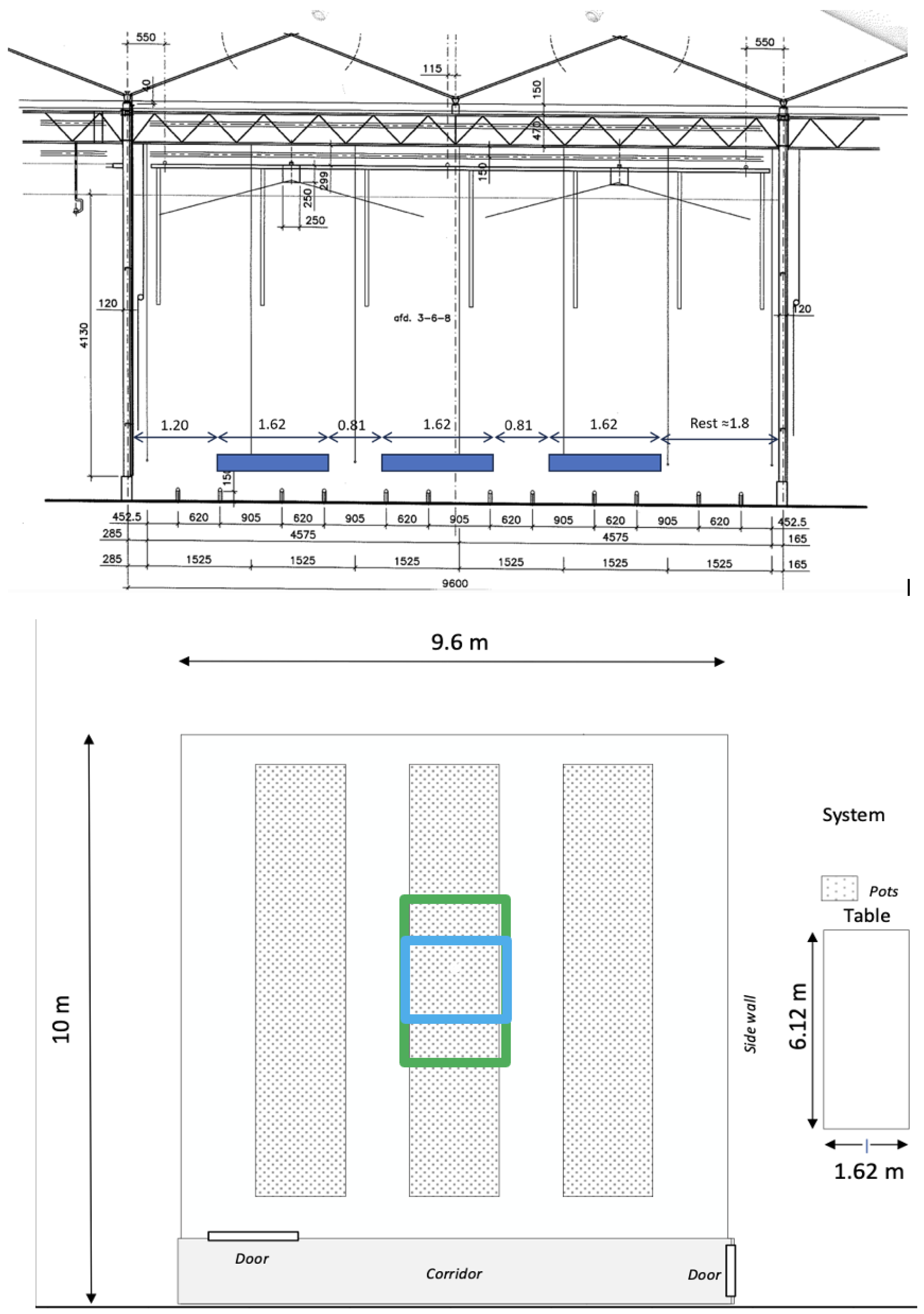
2.1. Experiment Setup
2.2. Greenhouse Compartments and Equipment
2.3. Sensors and Data Collection
2.4. Greenhouse Climate and Crop Control
- Algorithms could control the air temperature using the Heating Temperature Setpoint and the Ventilation Temperature Setpoint. The direct control of the Minimum Window Position and Heating Pipe Temperature was also possible.
- Increasing the humidity using fogging and reducing the humidity via ventilation were both controlled via the Humidity Deficit Setpoint, with a “deadzone” of /m3 before fogging.
- The concentration was controlled using the CO2 Concentration Setpoint.
- The LED lamps, as well as the screens, can be directly controlled by providing the Activation Percentage.
- Irrigation was steered by defining the Shot Interval, which is the time in seconds between subsequent shots of 1 min drip irrigation.
- Two crop actions, Plant Density (spacing) and the final Harvest Date, were provided via the same data interface, but executed once a day manually by our greenhouse staff.
2.5. Data Platform
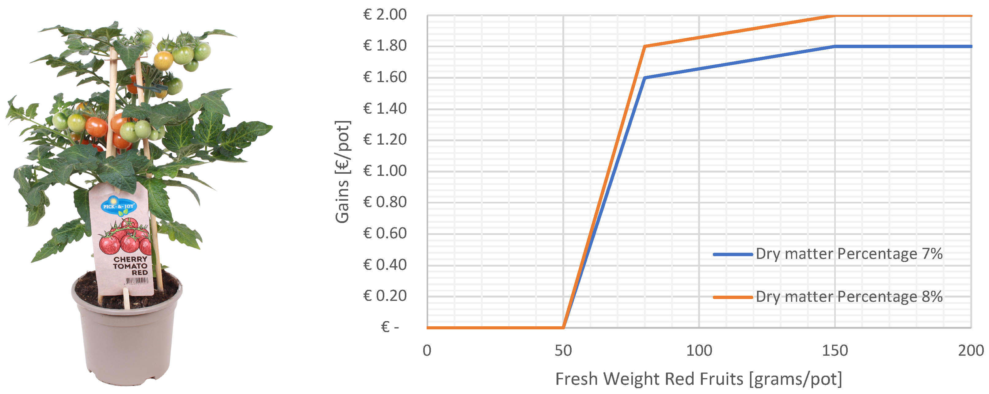
Cultivation Objective: Net Profit
2.6. Secondary Algorithm Evaluation Criteria: Robustness
3. Results
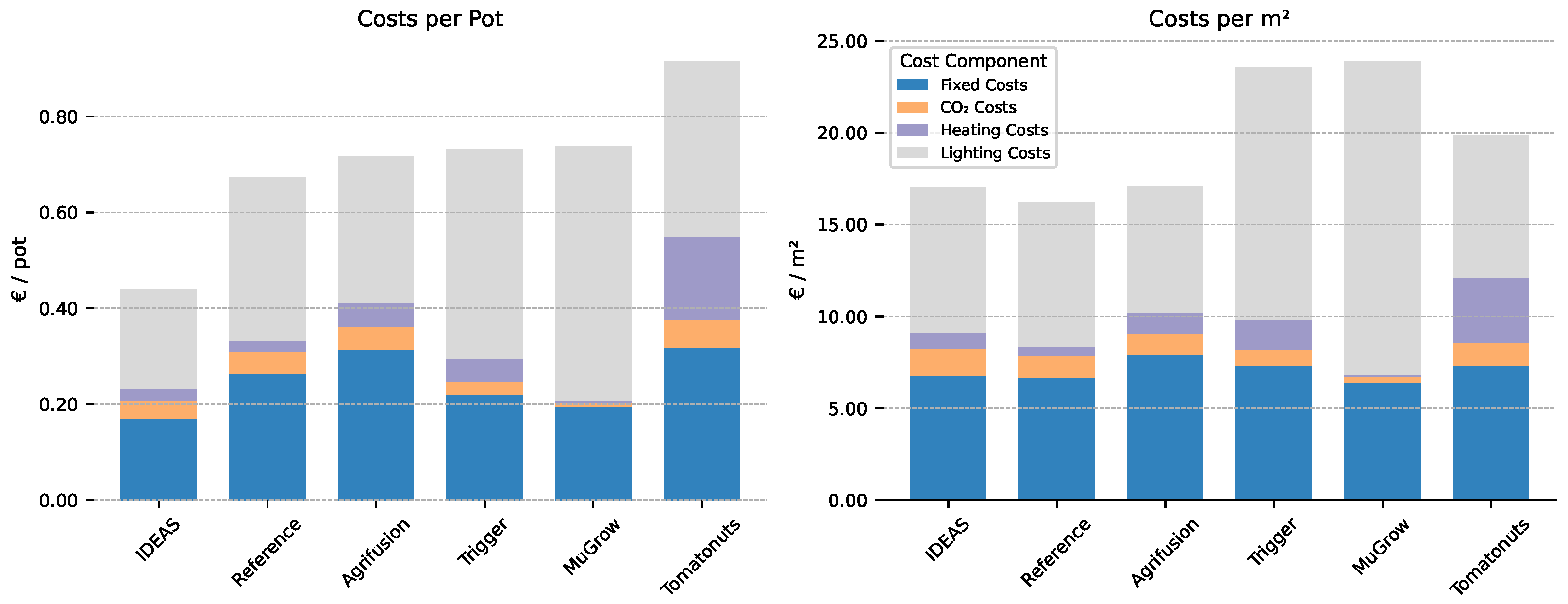
3.1. Net Profit
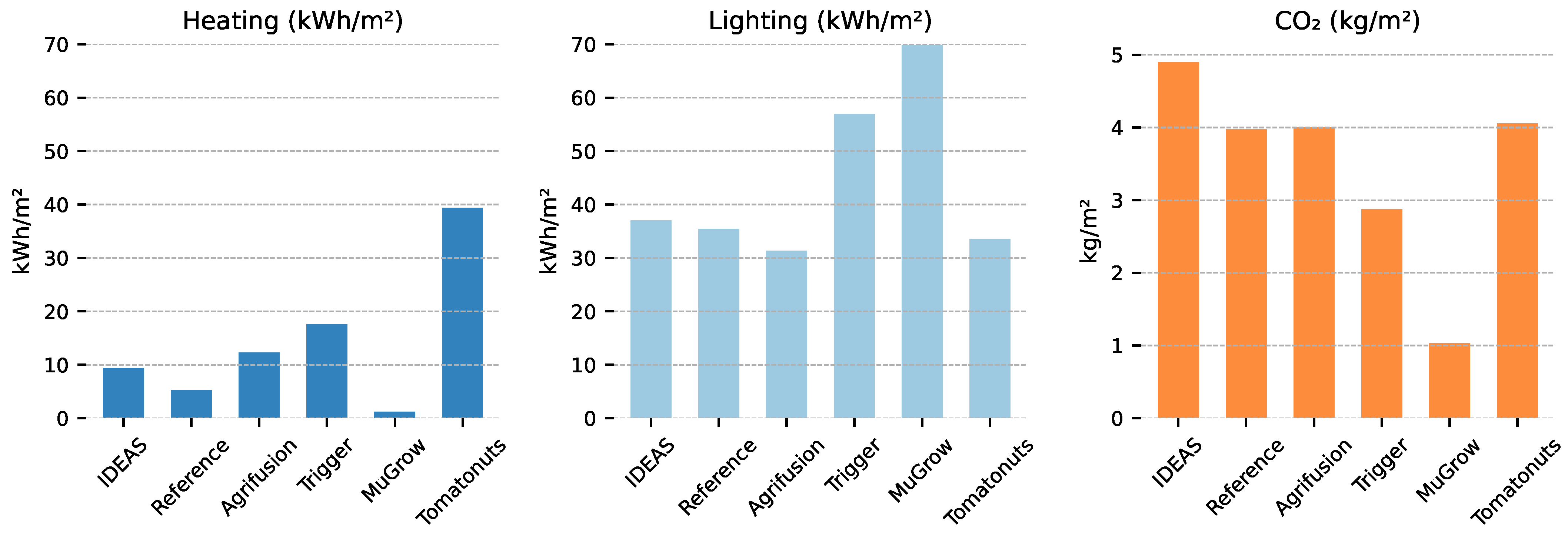
3.2. Climate Realization and Energy Usage
Light Use Efficiency
3.3. Crop Strategy
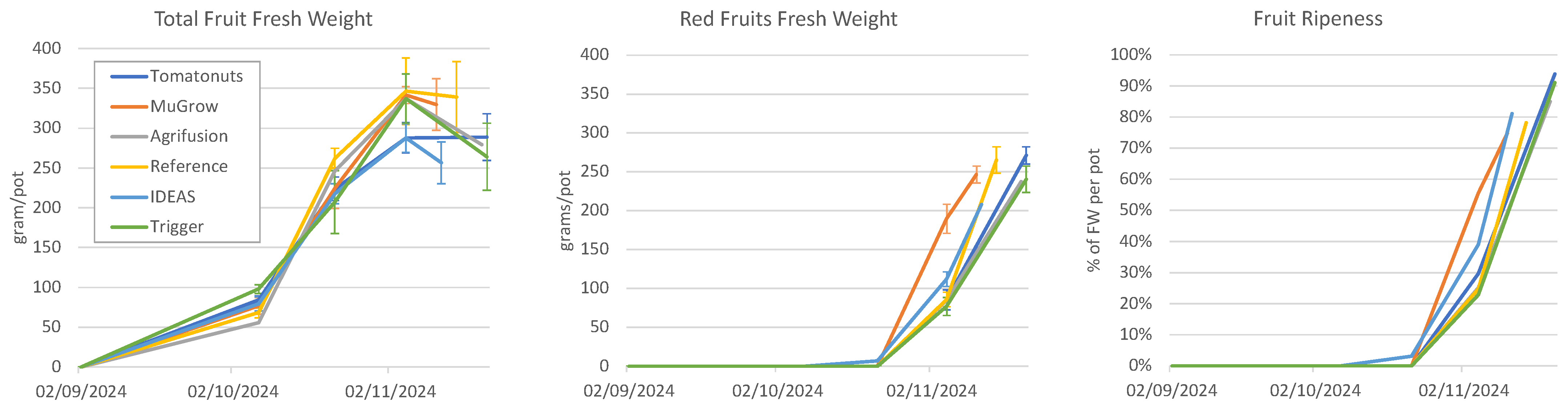
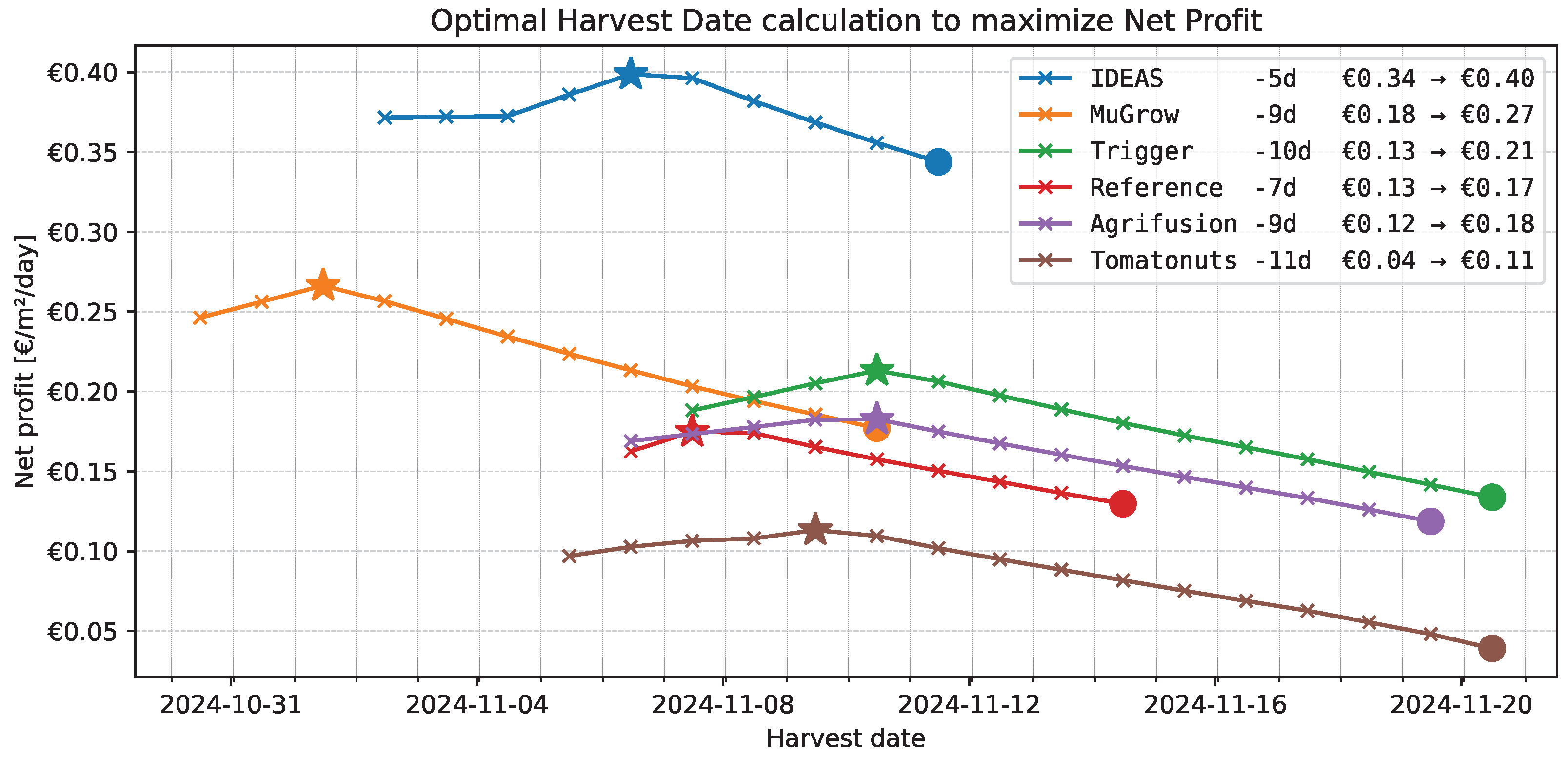
3.3.1. Harvest Moment
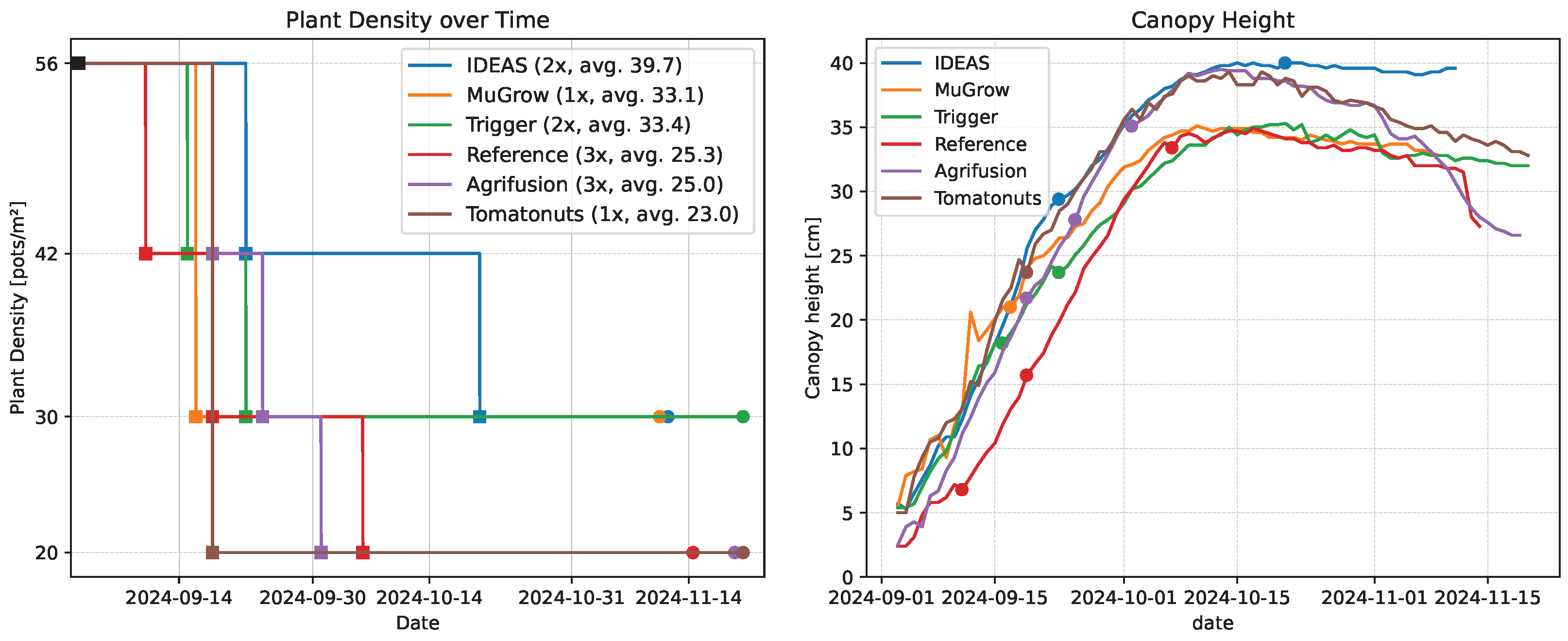
3.3.2. Plant Spacing
3.3.3. Feasibility as a Year-Round Production System
3.4. Autonomy and Robustness
4. Discussion
4.1. Net Profit
4.2. Light Use Efficiency
4.3. Optimal Harvest Moment
4.4. Plant Spacing
4.5. Feasibility as a Year-Round Production System
4.6. Robustness
4.7. Autonomy
5. Conclusions
Author Contributions
Funding
Institutional Review Board Statement
Informed Consent Statement
Data Availability Statement
Acknowledgments
Conflicts of Interest
Appendix A

| Parameter | Unit | Description |
|---|---|---|
| Heating temperature setpoint | °C | If the greenhouse air temperature falls below the this value, the heating pipes are activated. |
| Minimum pipe temperature | °C | Minimum temperature of the water flowing through the heating pipe. Allows for the direct control of heating without setpoints. |
| Ventilation temperature setpoint | °C | If the greenhouse air temperature rises above this value, the ventilation windows are opened. |
| Minimum window position | Forces the windows open, irregardless of the other controls. | |
| Concentration setpoint | ppm | If the concentration falls below this value, dosing is activated. The dosing rate is constant, so it is either on or off. |
| Humidity deficit setpoint | /m3 | Ventilation and fogging are both controlled via the humidity deficit (dx) setpoint. There is a “dead zone” of /m3 in between the two control actions. The vents are opened if the dx drops below the setpoint; fogging is activated if the dx is more than the dead zone above the setpoint. |
| Lamp activation percentage | [0, 10–100]% | The lights can either be set off, or dimmed between 10% and 100%. |
| Energy screen position | [0–100]% | 0 meaning the screen is not used. |
| Black-out screen position | [0–100]% | 0 meaning the screen is not used. The screen must be closed at night when the lamps are on, to prevent light pollution. |
| Irrigation shot interval | Minutes | The interval between subsequent irrigation shots. |
| Plant density | Pots/m2 | Allowed values: [56, 42, 30, 20]. Automatic spacing systems are commercially available, but in this small experimental setup, spacing is performed manually by the greenhouse staff. |
| Harvest day | Day number | The day (Jan 1st = 1) on which all plants should be harvested. Harvest is performed manually by our greenhouse staff. |
| Parameter | Unit | Description |
|---|---|---|
| Pipe temperature | °C | Temperature of the water flowing through the heating pipes. A higher temperature means faster heating of the greenhouse, but costs more heating energy. This value is 0 if there is no water flow. |
| Window position: Lee side | [0–100]% | When the greenhouse temperature is too high, the lee-side first opens. |
| Window position: Wind side | [0–100]% | If lee-side ventilation does not provide sufficient cooling, the wind side is also opened. |
| Cumulative dosage duration | minutes | Total minutes of dosage. Reset daily. |
| Irrigation Cumulative water flow duration | Minutes | Total minutes of irrigation. Reset daily. |
| Parameter | Unit | Description |
|---|---|---|
| Air temperature | °C | |
| Relative humidity | [0–100]% | |
| Humidity deficit | /m3 | |
| Concentration | ppm | |
| PAR light intensity | /m2 | |
| Drain volume | liter/10 pots | Because of the data-resolution, this quantity is calculated per 10 pots. |
| Drain EC | / | |
| Drain pH | - | |
| Soil temperature (3×) | °C | |
| Soil relative permittivity (3×) | - | |
| Soil bulk-EC (3×) | / | |
| Outside air temperature | °C | |
| Outside relative humidity | [0–100]% | |
| Outside absolute humidity | /m3 | |
| Outside PAR light intensity | /m2 | |
| Global radiation | /m2 | |
| Outside radiation sum | /cm2 | Reset daily |
| Wind speed | m/s | |
| Wind direction | 0–360° | 0 = north. |
| Rain state | 0–1 | 1 = rain, 0 = dry. |
| Heat emission | /m2 | Measured with a pyrgeometer. |
| Expected outside air temperature | °C | |
| Expected outside relative humidity | [0–100]% | |
| Expected global radiation | /m2 | |
| Expected global radiation Sum | /cm2 | Radiation sum expected for that day. |
| Expected degree of cloudiness | 1–8 |
| Team | Parameter | Unit | Sensor Brand and Description |
|---|---|---|---|
| Agrifusion | Plant weight scale | kg | Aranet—plant weight scale |
| Microclimate temperature | °C | Aranet—temperature | |
| Microclimate relative humidity | [0–100]% | Aranet—relative humidity | |
| Biosignals | Vivent—electrophysiology sensor | ||
| MuGrow | Efficiency of photosystem-II | % | Gardin—chlorophyll fluorescence camera |
| Photosynthetic capacity | % | Gardin—chlorophyll fluorescence camera | |
| Energy balance—light saturation | - | Gardin—chlorophyll fluorescence camera | |
| Electron transport | /m2 | Gardin—chlorophyll fluorescence camera | |
| Actinic—leaf response | - | Gardin—chlorophyll fluorescence camera | |
| Quantum yield—QE | - | Gardin—chlorophyll Fluorescence camera | |
| Trigger | Plant weight scale | g | Quantified sensor technology—firefly standing scale |
| Leaf temperature 1 | °C | Quantified sensor technology—firefly infrared thermometer | |
| Leaf temperature 2 | °C | Quantified sensor technology—firefly infrared thermometer |
References
- Stanghellini, C. Horticultural production in greenhouses: Efficient use of water. Acta Hortic. 2014, 1034, 25–32. [Google Scholar] [CrossRef]
- Graamans, L.; Baeza, E.; van den Dobbelsteen, A.; Tsafaras, I.; Stanghellini, C. Plant factories versus greenhouses: Comparison of resource use efficiency. Agric. Syst. 2018, 160, 31–43. [Google Scholar] [CrossRef]
- Rabo Research Food & Agribusiness. Positive Outlook for Greenhouse Production; Technical Report; Rabo Research Food & Agribusiness: New York, NY, USA, 2025. [Google Scholar]
- Heuvelink, E.; Hemming, S.; Marcelis, L.F. Some recent developments in controlled-environment agriculture: On plant physiology, sustainability, and autonomous control. J. Hortic. Sci. Biotechnol. 2025. [CrossRef]
- Pearson, S. Artificial intelligence in horticulture. J. Hortic. Sci. Biotechnol. 2025, 1–7. [Google Scholar] [CrossRef]
- Hemming, J.; Balendonck, J. Advances in the use of robotics in greenhouse cultivation. In Advances in the Use of Robotics in Greenhouse Cultivation; Burleigh Dodds Science Pulibshing: Cambridge, UK, 2024; pp. 635–660. [Google Scholar] [CrossRef]
- van Straten, G.; van Willigenburg, G.; van Henten, E.; van Ooteghem, R. Optimal control of greenhouse cultivation. Optim. Control Greenh. Cultiv. 2010, 1–297. [Google Scholar] [CrossRef]
- de Zwart, H.F. Analyzing Energy-Saving Options in Greenhouse Cultivation Using a Simulation Model. Ph.D. Thesis, Wageningen University, Wageningen, The Netherland, 1996. [Google Scholar] [CrossRef]
- Katzin, D.; van Henten, E.J.; van Mourik, S. Process-based greenhouse climate models: Genealogy, current status, and future directions. Agric. Syst. 2022, 198, 103388. [Google Scholar] [CrossRef]
- Hemming, S.; De Zwart, F.; Elings, A.; Righini, I.; Petropoulou, A. Remote Control of Greenhouse Vegetable Production with Artificial Intelligence—Greenhouse Climate, Irrigation, and Crop Production. Sensors 2019, 19, 1807. [Google Scholar] [CrossRef]
- Hemming, S.; de Zwart, F.; Elings, A.; Petropoulou, A.; Righini, I. Cherry Tomato Production in Intelligent Greenhouses—Sensors and AI for Control of Climate, Irrigation, Crop Yield, and Quality. Sensors 2020, 20, 6430. [Google Scholar] [CrossRef]
- Petropoulou, A.S.; van Marrewijk, B.; de Zwart, F.; Elings, A.; Bijlaard, M.; van Daalen, T.; Jansen, G.; Hemming, S. Lettuce Production in Intelligent Greenhouses—3D Imaging and Computer Vision for Plant Spacing Decisions. Sensors 2023, 23, 2929. [Google Scholar] [CrossRef]
- An, Z.; Cao, X.; Yao, Y.; Zhang, W.; Li, L.; Wang, Y.; Guo, S.; Luo, D. A Simulator-based Planning Framework for Optimizing Autonomous Greenhouse Control Strategy. In Proceedings of the Thirty-First International Conference on Automated Planning and Scheduling (ICAPS 2021), Guangzhou, China, 7–12 June 2021. [Google Scholar]
- Cao, X.; Yao, Y.; Li, L.; Zhang, W.; An, Z.; Zhang, Z.; Xiao, L.; Guo, S.; Cao, X.; Wu, M.; et al. iGrow: A Smart Agriculture Solution to Autonomous Greenhouse Control. In Proceedings of the Thirty-Sixth AAAI Conference on Artificial Intelligence (AAAI-22), Online, 22 February–1 March 2022. [Google Scholar] [CrossRef]
- Zhang, W.; Cao, X.; Yao, Y.; An, Z.; Xiao, X.; Luo, D. Robust Model-based Reinforcement Learning for Autonomous Greenhouse Control. Proc. Mach. Learn. Res. 2021, 157. [Google Scholar]
- Laouz, H.; Soheyb, A.; Labib, S.T.; Benharkat, A.N.; Samir, M. Performance and Robustness Analysis of Advanced Machine Learning Models for Predicting the Required Irrigation Water Amount. Int. J. Comput. Digit. Syst. 2024, 16. [Google Scholar] [CrossRef]
- Lin, Z.; Fu, R.; Ren, G.; Zhong, R.; Ying, Y.; Lin, T. Automatic monitoring of lettuce fresh weight by multi-modal fusion based deep learning. Front. Plant Sci. 2022, 13, 980581. [Google Scholar] [CrossRef] [PubMed]
- Gang, M.S.; Kim, H.J.; Kim, D.W. Estimation of Greenhouse Lettuce Growth Indices Based on a Two-Stage CNN Using RGB-D Images. Sensors 2022, 22, 5499. [Google Scholar] [CrossRef]
- Hou, L.; Zhu, Y.; Wang, M.; Wei, N.; Dong, J.; Tao, Y.; Zhou, J.; Zhang, J. Multimodal Data Fusion for Precise Lettuce Phenotype Estimation Using Deep Learning Algorithms. Plants 2024, 13, 3217. [Google Scholar] [CrossRef] [PubMed]
- Cruz, S.; van Santen, E.; Gómez, C. Evaluation of Compact Tomato Cultivars for Container Gardening Indoors and under Sunlight. Horticulturae 2022, 8, 294. [Google Scholar] [CrossRef]
- Karpe, M.; Marcelis, L.F.; Heuvelink, E. Dynamic plant spacing in tomato results in high yields while mitigating the reduction in fruit quality associated with high planting densities. Front. Plant Sci. 2024, 15, 1386950. [Google Scholar] [CrossRef]
- Niu, Y.; Lyu, H.; Liu, X.; Zhang, M.; Li, H. Photosynthesis prediction and light spectra optimization of greenhouse tomato based on response of red–blue ratio. Sci. Hortic. 2023, 318, 112065. [Google Scholar] [CrossRef]
- Hogewoning, S.W.; Trouwborst, G.; Meinen, E.; Van Ieperen, W. Finding the optimal growth-light spectrum for greenhouse crops. Proc. Acta Hortic. Int. Soc. Hortic. Sci. 2012, 956, 357–363. [Google Scholar] [CrossRef]
- Heuvelink, E. Effect of plant density on biomass allocation to the fruits in tomato (Lycopersicon esculentum Mill.). Sci. Hortic. 1995, 64, 193–201. [Google Scholar] [CrossRef]
- Amundson, S.; Deyton, D.E.; Kopsell, D.A.; Hitch, W.; Moore, A.; Sams, C.E. Optimizing plant density and production systems to maximize yield of greenhouse-grown ‘Trust’ tomatoes. HortTechnology 2012, 22, 44–48. [Google Scholar] [CrossRef]
- Cockshull, K.E.; Ho, L.C. Regulation of tomato fruit size by plant density and truss thinning. J. Hortic. Sci. 1995, 70, 395–407. [Google Scholar] [CrossRef]
- Testa, R.; di Trapani, A.M.; Sgroi, F.; Tudisca, S. Economic Sustainability of Italian Greenhouse Cherry Tomato. Sustainability 2014, 6, 7967–7981. [Google Scholar] [CrossRef]


| Algorithm | Red Fruit Fresh Weight [g/pot] | Red Fruit Dry Weight [%] | Red Fruits [%] | Gains [EUR/pot] | Costs [EUR/pot] | Cultivation Duration [Days] | Avg. Plant Density [pots/m2] | Net Profit [EUR/m2/day] |
|---|---|---|---|---|---|---|---|---|
| IDEAS | 219 | 6.8% | 86% | 1.05 | −0.44 | 70 | 39.7 | 0.34 |
| MuGrow | 252 | 7.3% | 76% | 1.11 | −0.74 | 70 | 33.1 | 0.18 |
| Trigger | 268 | 5.9% | 101% | 1.05 | −0.73 | 80 | 33.4 | 0.13 |
| Reference | 275 | 6.6% | 81% | 1.05 | −0.67 | 74 | 25.3 | 0.13 |
| Agrifusion | 258 | 7.2% | 92% | 1.09 | −0.72 | 78 | 25.0 | 0.12 |
| Tomatonuts | 283 | 6.0% | 98% | 1.05 | −0.91 | 80 | 23.0 | 0.04 |
| Daily Average Temperature [°C] | Daily PAR Sum [mol/day] | Daily Average CO2 Concentration [ppm] | Daily Total Irrigation [mL/pot] | |
|---|---|---|---|---|
| Agrifusion | 20.6 | 9.8 | 678 | 36.5 |
| IDEAS | 21.8 | 11.3 | 708 | 65.8 |
| MuGrow | 21.4 | 17.0 | 567 | 50.2 |
| Reference | 20.4 | 11.0 | 770 | 55.2 |
| Tomatonuts | 21.2 | 9.6 | 725 | 73.6 |
| Trigger | 20.0 | 13.2 | 503 | 92.7 |
Disclaimer/Publisher’s Note: The statements, opinions and data contained in all publications are solely those of the individual author(s) and contributor(s) and not of MDPI and/or the editor(s). MDPI and/or the editor(s) disclaim responsibility for any injury to people or property resulting from any ideas, methods, instructions or products referred to in the content. |
© 2025 by the authors. Licensee MDPI, Basel, Switzerland. This article is an open access article distributed under the terms and conditions of the Creative Commons Attribution (CC BY) license (https://creativecommons.org/licenses/by/4.0/).
Share and Cite
Maree, S.C.; Zhang, P.; van Marrewijk, B.M.; de Zwart, F.; Bijlaard, M.; Hemming, S. Autonomous Greenhouse Cultivation of Dwarf Tomato: Performance Evaluation of Intelligent Algorithms for Multiple-Sensor Feedback. Sensors 2025, 25, 4321. https://doi.org/10.3390/s25144321
Maree SC, Zhang P, van Marrewijk BM, de Zwart F, Bijlaard M, Hemming S. Autonomous Greenhouse Cultivation of Dwarf Tomato: Performance Evaluation of Intelligent Algorithms for Multiple-Sensor Feedback. Sensors. 2025; 25(14):4321. https://doi.org/10.3390/s25144321
Chicago/Turabian StyleMaree, Stef C., Pinglin Zhang, Bart M. van Marrewijk, Feije de Zwart, Monique Bijlaard, and Silke Hemming. 2025. "Autonomous Greenhouse Cultivation of Dwarf Tomato: Performance Evaluation of Intelligent Algorithms for Multiple-Sensor Feedback" Sensors 25, no. 14: 4321. https://doi.org/10.3390/s25144321
APA StyleMaree, S. C., Zhang, P., van Marrewijk, B. M., de Zwart, F., Bijlaard, M., & Hemming, S. (2025). Autonomous Greenhouse Cultivation of Dwarf Tomato: Performance Evaluation of Intelligent Algorithms for Multiple-Sensor Feedback. Sensors, 25(14), 4321. https://doi.org/10.3390/s25144321