

An Efficient SAR Raw Signal Simulator Accounting for Large Trajectory Deviation


Abstract
1. Introduction
2. Model of the Proposed Method
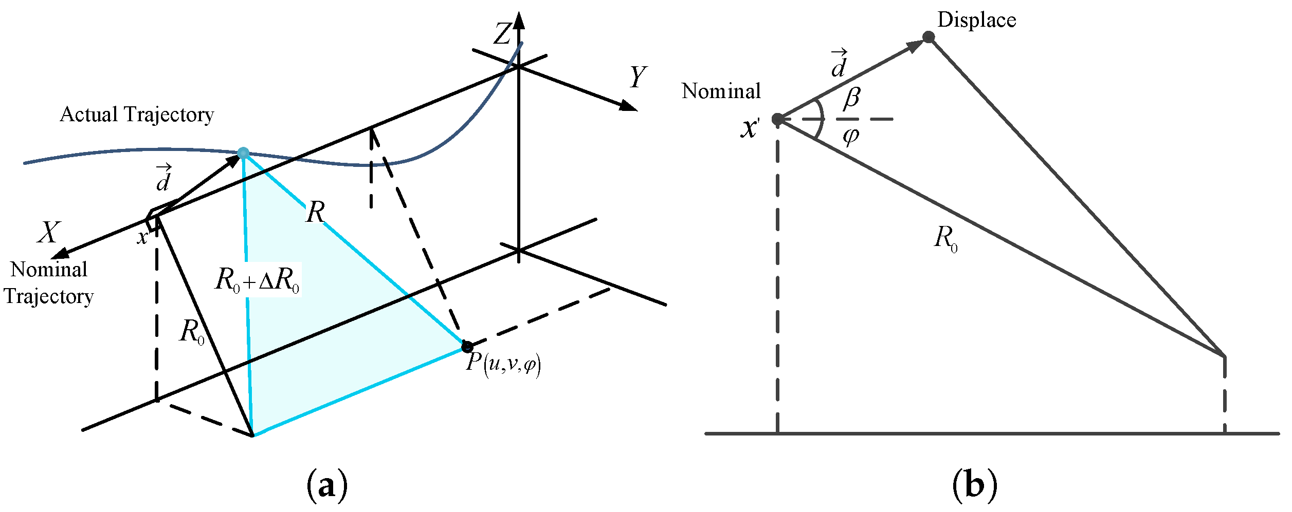
2.1. Geometry of SAR System with Trajectory Deviation
- the azimuth and (slant) range coordinates of the scene generic scattering point P;
- the azimuth and (slant) range coordinates of the antenna;
- pitch angle of the platform;
- R the target-to-antenna distances in the generic antenna position for actual trajectories;
- the closest range to the nominal trajectory (in nominal trajectory, ).
2.2. Model of SAR Raw Signal
- is the radar’s instantaneous location;
- , with as frequency and c as the wave propagation speed;
- is the transmitted radar signal;
- is the SAR transfer function:
- Spatial Representation: the SAR raw signal is viewed as a function of radar location rather than the conventional fast time (slant range) and slow time (azimuth). This is particularly suitable for handling nonlinear radar trajectories.
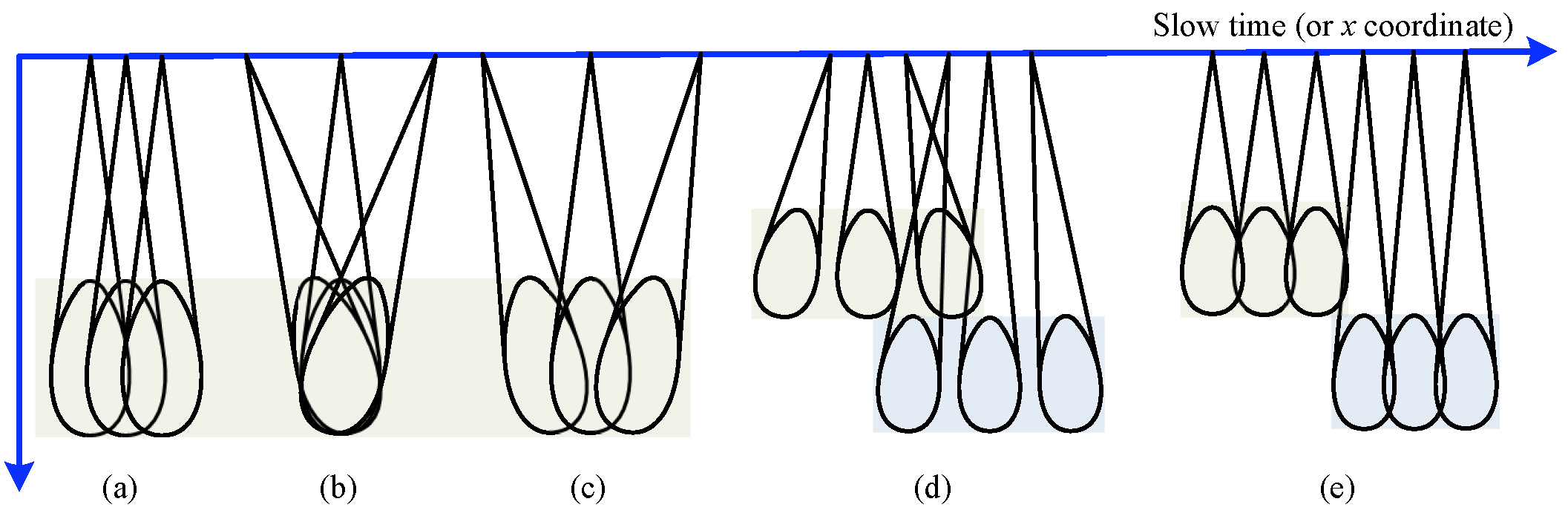
- Applicability to Multiple Modes: the model applies to various SAR acquisition modes. For instance, a constant corresponds to stripmap mode, while variable enables modes like sliding spotlight or TOPSAR (see Figure 2).
- Factorized Structure: the SAR signal is split into scatterer-independent and scatterer-dependent . Efficient computation of is key to simulator design.
3. Theory of the Proposed Method
3.1. Mathematical Principle
- (1)
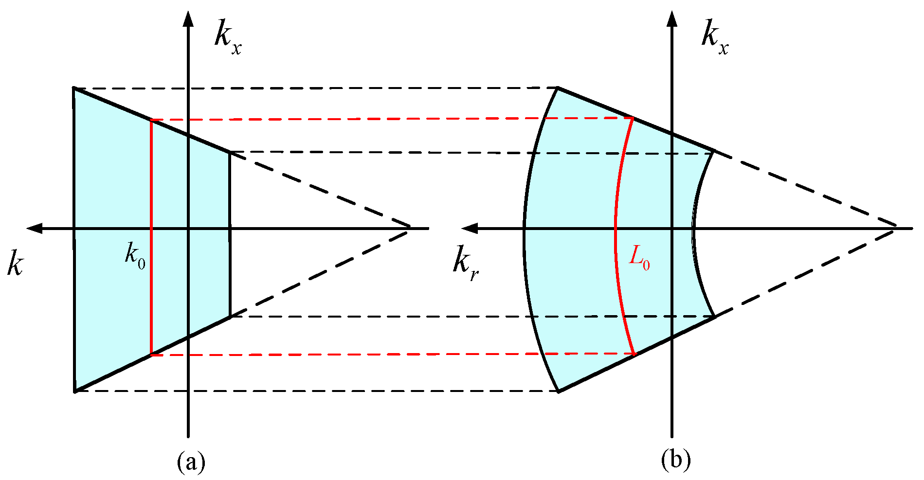
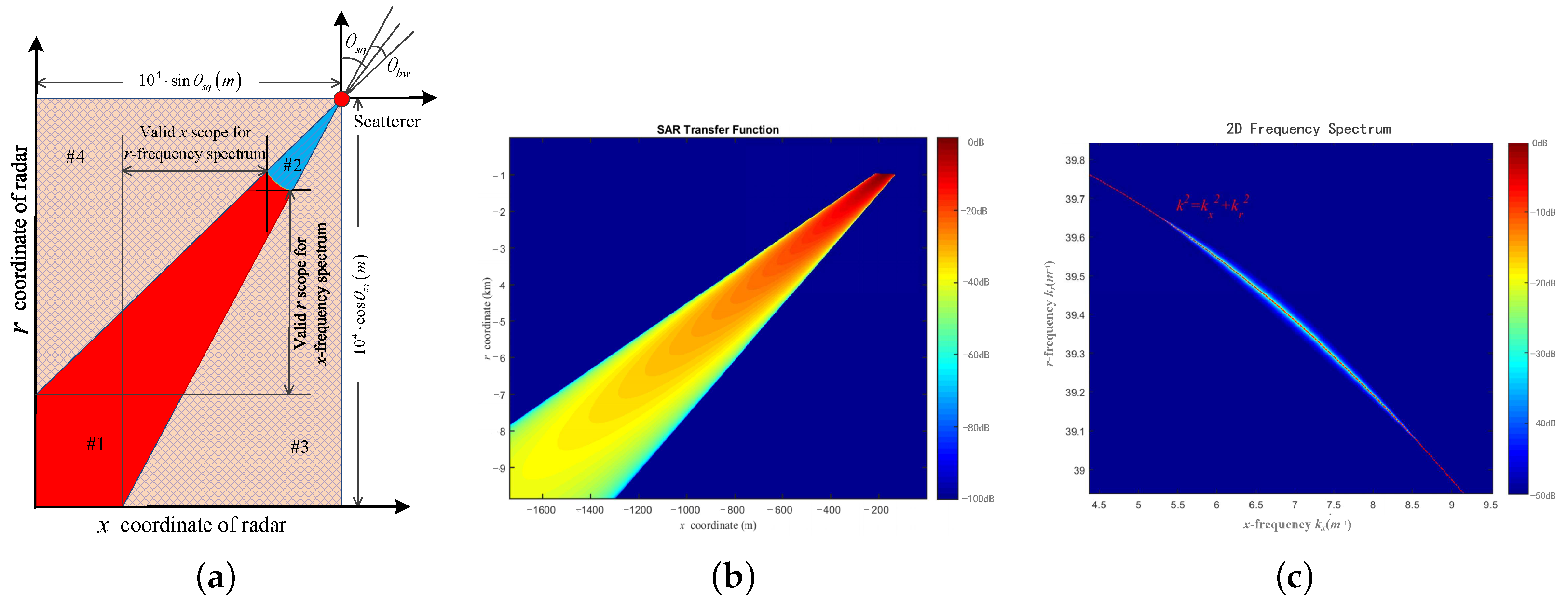
- L is the arc on circle , which satisfieswhere denotes the angle in the Cartesian coordinates . This integral interval is because the 2D spatial frequency spectrum of the transfer function is band-limited, as illustrated in Figure 3. Note that the integral is along the direction of growth.
- (2)
- is relevant to the bandwidth and beam pattern, and can be expressed as follows:The rectangular window is obtained from the fact that the bandwidth of the transmitted signal is limited. As shown in Figure 3, the radius in domain represents the wavenumber k. According to , the bandwidth is B with the carrier frequency . Furthermore, the 2D spatial frequency spectrum of depends on the beam pattern of the radar beam. As illustrated by the window function , the spectrum of transfer function is modulated by the beam pattern .
- (3)
- is the correction termwhere is a constant irrelevant to this work. Further, the exponential term is obtained from the trajectory deviation.
- (4)
- is the 2D Fourier transform of weighted by .
3.2. Implementation
4. Performance Analysis of the Method
4.1. Computational Complexity
- Weighting the reflectivity map requires FLOPs, where and are the number of scatterers in the azimuth and range directions, respectively. Furthermore, the 2D FFT operation of modulated backscattering coefficient requires FLOPs.
- Spectrum extraction and interpolation along the azimuth frequency require FLOPs, where is the sampling number of SAR raw signal in the range direction and is the length of the interpolation kernel.
- Antenna pattern modulation and spectrum correction can be applied together. This operation is a complex multiplication and requires FLOPs at the instantaneous location . For the entire trajectory, these operations should be repeated for each position and require FLOPs, where is the sampling number of SAR raw signal in the azimuth direction.
- At the instantaneous location , the integration should be repeated times for each k and thus requires FLOPs. In order to obtain for the entire trajectory, we should apply the integral operation for each . Therefore, the integral operation for the entire trajectory requires FLOPs.
- One-dimensional FFT operation and complex multiplication require FLOPs and FLOPs, respectively. Finally, 1D IFFT operation requires , because this operation should be repeated at each .
4.2. Flexibility
4.3. Error Analysis and Limitations
4.4. Application to Bistatic SAR
5. Simulation Results
5.1. Verification of Spatial Spectrum Analysis
5.2. Results of Stripmap SAR for Point Scatterer Case
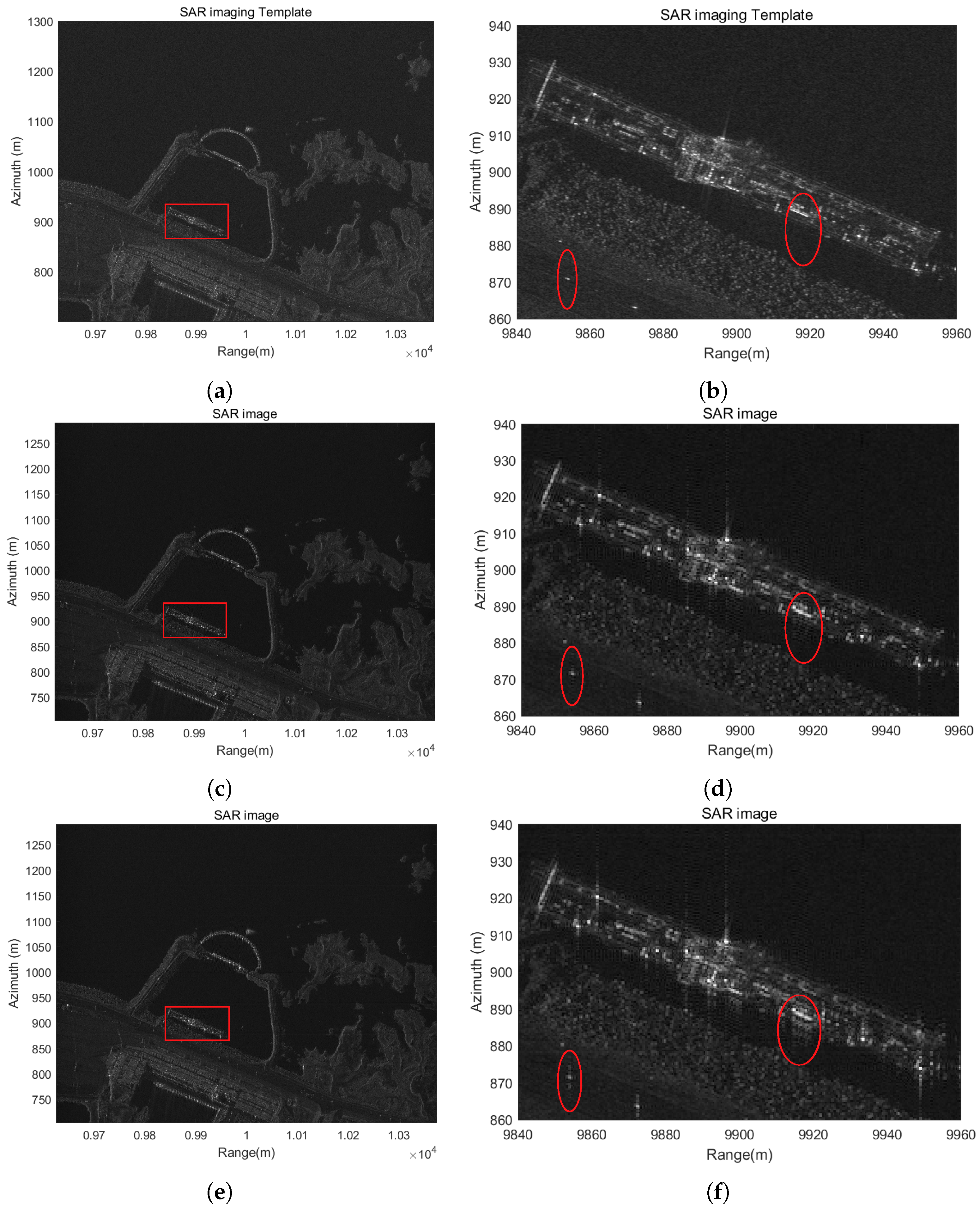
5.3. Results of Stripmap SAR for General Electromagnetic Case
5.4. Results of Spotlight SAR with Trajectory Deviation
6. Conclusions
Author Contributions
Funding
Institutional Review Board Statement
Informed Consent Statement
Data Availability Statement
Conflicts of Interest
Appendix A
Appendix A.1. Derivation of the Spatial Spectrum
Appendix A.2. Derivation of the Method
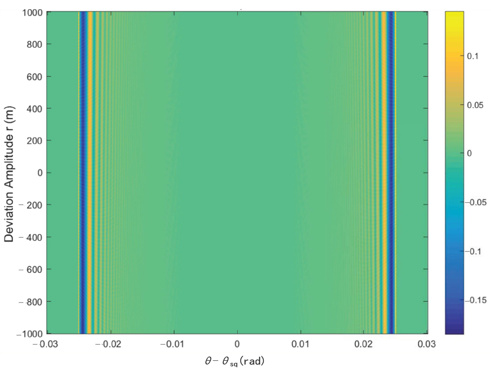
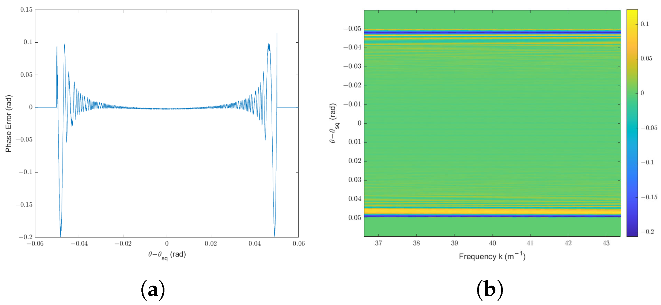
Appendix A.3. The Simulation of the Error Analysis
References
- Zhang, M.; Meng, Z.; Wang, G.; Xue, Y. Range-Dependent Channel Calibration for High-Resolution Wide-Swath Synthetic Aperture Radar Imagery. Sensors 2024, 24, 3278. [Google Scholar] [CrossRef] [PubMed]
- Franceschetti, G.; Rozzi, T.; Pierantoni, L.; Massaro, A. An innovative model of electromagnetic propagation in the urban environment. In Proceedings of the IEEE Antennas and Propagation Society International Symposium, Albuquerque, NM, USA, 9–14 July 2006; pp. 3495–3498. [Google Scholar] [CrossRef]
- Franceschetti, G.; Iodice, A.; Riccio, D.; Ruello, G.; Siviero, R. SAR raw signal simulation of oil slicks in ocean environments. IEEE Trans. Geosci. Remote Sens. 2002, 40, 1935–1949. [Google Scholar] [CrossRef]
- Franceschetti, G.; Iodice, A.; Riccio, D.; Ruello, G. Oil slicks on the ocean surface: A SAR raw signal simulator. In Proceedings of the US/EU Baltic International Symposium, Klaipeda, Lithuania, 23–26 May 2006; IEEE: Piscataway, NJ, USA, 2006; pp. 1–6. [Google Scholar] [CrossRef]
- Zeng, T.; Hu, C.; Sun, H.; Chen, E. A Novel Rapid SAR Simulator Based on Equivalent Scatterers for Three-Dimensional Forest Canopies. IEEE Trans. Geosci. Remote Sens. 2014, 52, 5243–5255. [Google Scholar] [CrossRef]
- Franceschetti, G.; Guida, R.; Iodice, A.; Riccio, D.; Ruello, G. Efficient Simulation of hybrid stripmap/spotlight SAR raw signals from extended scenes. IEEE Trans. Geosci. Remote Sens. 2004, 42, 2385–2396. [Google Scholar] [CrossRef]
- Liu, Y.; Wang, W.; Dai, S.; Rao, B.; Wang, G. A Unified Multimode SAR Raw Signal Simulation Method Based on Acquisition Mode Mutation. IEEE Geosci. Remote Sens. Lett. 2017, 14, 1233–1237. [Google Scholar] [CrossRef]
- Mittermayer, J.; Lord, R.; Borner, E. Sliding spotlight SAR processing for TerraSAR-X using a new formulation of the extended chirp scaling algorithm. In Proceedings of the IEEE International Geoscience and Remote Sensing Symposium (IGARSS ’03), Toulouse, France, 21–25 July 2003; Volume 3, pp. 1462–1464. [Google Scholar] [CrossRef]
- Xu, W.; Deng, Y.; Feng, F.; Liu, Y.; Li, G. TOPS Mode Raw Data Generation From Wide-Beam SAR Imaging Modes. IEEE Geosci. Remote Sens. Lett. 2012, 9, 720–724. [Google Scholar] [CrossRef]
- Qiu, X.; Hu, D.; Zhou, L.; Ding, C. A Bistatic SAR Raw Data Simulator Based on Inverse ω-k Algorithm. IEEE Trans. Geosci. Remote Sens. 2010, 48, 1540–1547. [Google Scholar]
- Liu, Y.; Deng, Y.; Wang, R.; Yan, H.; Chen, J. Efficient and precise frequency-modulated continuous wave synthetic aperture radar raw signal simulation approach for extended scenes. Radar Sonar Navig. IET 2012, 6, 858–866. [Google Scholar] [CrossRef]
- Luo, Y.; Song, H.; Wang, R.; Deng, Y.; Zheng, S. An Accurate and Efficient Extended Scene Simulator for FMCW SAR with Static and Moving Targets. IEEE Geosci. Remote Sens. Lett. 2014, 11, 1672–1676. [Google Scholar] [CrossRef]
- Mori, A.; De Vita, F. A time-domain raw signal Simulator for interferometric SAR. IEEE Trans. Geosci. Remote Sens. 2004, 42, 1811–1817. [Google Scholar] [CrossRef]
- Zhang, J.; Zeng, Y.; Qi, Z.; Wang, L.; Wang, Y.; Shen, X. Two-Dimensional Barrage Jamming against SAR Using a Frequency Diverse Array Jammer. Sensors 2023, 23, 2449. [Google Scholar] [CrossRef] [PubMed]
- Liu, Y.; Wang, W.; Pan, X.; Fu, Q.; Wang, G. Inverse Omega-K Algorithm for the Electromagnetic Deception of Synthetic Aperture Radar. IEEE J. Sel. Top. Appl. Earth Obs. Remote Sens. 2016, 9, 3037–3049. [Google Scholar] [CrossRef]
- Franceschetti, G.; Migliaccio, M.; Riccio, D. SAR raw signal simulation of actual ground sites described in terms of sparse input data. IEEE Trans. Geosci. Remote Sens. 1994, 32, 1160–1169. [Google Scholar] [CrossRef]
- Meng, D.; Hu, D.; Ding, C. Precise Focusing of Airborne SAR Data with Wide Apertures Large Trajectory Deviations: A Chirp Modulated Back-Projection Approach. IEEE Trans. Geosci. Remote Sens. 2015, 53, 2510–2519. [Google Scholar] [CrossRef]
- Li, Z.; Xing, M.; Xing, W.; Liang, Y.; Gao, Y.; Dai, B.; Hu, L.; Bao, Z. A Modified Equivalent Range Model and Wavenumber-Domain Imaging Approach for High-Resolution-High-Squint SAR with Curved Trajectory. IEEE Trans. Geosci. Remote Sens. 2017, 55, 3721–3734. [Google Scholar] [CrossRef]
- Franceschetti, G.; Iodice, A.; Perna, S.; Riccio, D. SAR Sensor Trajectory Deviations: Fourier Domain Formulation and Extended Scene Simulation of Raw Signal. IEEE Trans. Geosci. Remote Sens. 2006, 44, 2323–2334. [Google Scholar] [CrossRef]
- Franceschetti, G.; Iodice, A.; Perna, S.; Riccio, D. Efficient simulation of airborne SAR raw data of extended scenes. IEEE Trans. Geosci. Remote Sens. 2006, 44, 2851–2860. [Google Scholar] [CrossRef]
- Khwaja, A.; Ferro-Famil, L.; Pottier, E. Efficient Stripmap SAR Raw Data Generation Taking Into Account Sensor Trajectory Deviations. IEEE Geosci. Remote Sens. Lett. 2011, 8, 794–798. [Google Scholar] [CrossRef]
- Liu, Y.; Wang, W.; Pan, X.; Gu, Z.; Wang, G. Raw Signal Simulator for SAR with Trajectory Deviation Based on Spatial Spectrum Analysis. IEEE Trans. Geosci. Remote Sens. 2017, 55, 6651–6665. [Google Scholar] [CrossRef]
- Franceschetti, G.; Lanari, R. Synthetic Aperture Radar Processing; CRC Press: Boca Raton, FL, USA, 1999. [Google Scholar]
- Cumming, I.G.; Wong, F.H. Digital Processing of Synthetic Aperture Radar Data: Algorithms and Implementation; Artech House: Norwood, MA, USA, 2005. [Google Scholar]
- Xiuhe, L.; Yang, S.; Zhongwei, L.; Shunkai, Z.; Qianqian, S.; Shaoqi, D. Towards Order-Preserving and Zero-Copy Communication on Shared Memory for Large Scale Simulation. Chin. J. Electron. 2023, 32, 1066–1076. [Google Scholar] [CrossRef]
- Prats, P.; Scheiber, R.; Mittermayer, J.; Meta, A.; Moreira, A. Processing of Sliding Spotlight and TOPS SAR Data Using Baseband Azimuth Scaling. IEEE Trans. Geosci. Remote Sens. 2010, 48, 770–780. [Google Scholar] [CrossRef]
- Huai, Y.; Liang, Y.; Ding, J.; Xing, M.; Zeng, L.; Li, Z. An Inverse Extended Omega-K Algorithm for SAR Raw Data Simulation with Trajectory Deviations. IEEE Geosci. Remote Sens. Lett. 2016, 13, 826–830. [Google Scholar] [CrossRef]
- Rosen, P.A.; Hensley, S.; Joughin, I.R.; Li, F.K.; Madsen, S.N.; Rodriguez, E.; Goldstein, R.M. Synthetic aperture radar interferometry. Proc. IEEE 2000, 88, 333–382. [Google Scholar] [CrossRef]


| Parameter Type | Value |
|---|---|
| resolution | ≈0.5 m (both range and azimuth) |
| carrier frequency | 6.0 GHz, = 40 |
| bandwidth | = 300 MHz, |
| squint angle | = 0 rad |
| azimuth beam width | = 0.05 rad |
| azimuth beam pattern | , |
| is the angle between and |
| Parameter Type | Value |
|---|---|
| resolution | ≈0.15 m (range) |
| carrier frequency | 6.0 GHz, = 40 m−1 |
| bandwidth | = 1 GHz, = 6.67 m−1 |
| antenna rotation center | (0, 15) km |
| azimuth beam width | = 0.05 rad |
| azimuth beam pattern | , |
| where is the angle between and |
Disclaimer/Publisher’s Note: The statements, opinions and data contained in all publications are solely those of the individual author(s) and contributor(s) and not of MDPI and/or the editor(s). MDPI and/or the editor(s) disclaim responsibility for any injury to people or property resulting from any ideas, methods, instructions or products referred to in the content. |
© 2025 by the authors. Licensee MDPI, Basel, Switzerland. This article is an open access article distributed under the terms and conditions of the Creative Commons Attribution (CC BY) license (https://creativecommons.org/licenses/by/4.0/).
Share and Cite
Dai, S.; Zhang, H.; Wang, C.; Lin, Z.; Zhang, Y.; Ran, J. An Efficient SAR Raw Signal Simulator Accounting for Large Trajectory Deviation. Sensors 2025, 25, 4260. https://doi.org/10.3390/s25144260
Dai S, Zhang H, Wang C, Lin Z, Zhang Y, Ran J. An Efficient SAR Raw Signal Simulator Accounting for Large Trajectory Deviation. Sensors. 2025; 25(14):4260. https://doi.org/10.3390/s25144260
Chicago/Turabian StyleDai, Shaoqi, Haiyan Zhang, Cheng Wang, Zhongwei Lin, Yi Zhang, and Jinhe Ran. 2025. "An Efficient SAR Raw Signal Simulator Accounting for Large Trajectory Deviation" Sensors 25, no. 14: 4260. https://doi.org/10.3390/s25144260
APA StyleDai, S., Zhang, H., Wang, C., Lin, Z., Zhang, Y., & Ran, J. (2025). An Efficient SAR Raw Signal Simulator Accounting for Large Trajectory Deviation. Sensors, 25(14), 4260. https://doi.org/10.3390/s25144260