Abstract
This study presents an adaptive sliding mode control strategy tailored for robotic manipulators, featuring a quasi-convex function-based control gain and a time-delay estimation (TDE) enhanced by neural networks. To compensate for TDE errors, the proposed method utilizes both the previous TDE error and radial basis function neural networks with a weight update law that includes damping terms to prevent divergence. Additionally, a continuous gain function that is quasi-convex function dependent on the magnitude of the sliding variable is proposed to replace the traditional switching control gain. This continuous function-based gain has effectiveness in suppressing chattering phenomenon while guaranteeing the stability of the robotic manipulator in terms of uniform ultimate boundedness, which is demonstrated through both simulation and experiment results.
1. Introduction
Robotic manipulators have been increasingly employed across various fields, including manufacturing [1], surgery [2], service industries [3], and agriculture [4], due to their high versatility. To operate effectively across diverse fields, robotic manipulators must exhibit high accuracy and reliability, which requires precise model information for their nonlinear dynamics. However, highly nonlinear properties, external disturbances, and inaccuracies in system modeling make it difficult to obtain precise model information. Consequently, researchers have explored diverse control approaches including time-delay control (TDC) [5,6,7,8] and sliding mode control (SMC) [5,9,10,11,12,13] to cope with these issues.
In real environments, obtaining exact dynamic equations of robotic manipulators is challenging work due to inaccuracies in system modeling and external disturbances. Thus, a TDC technique utilizes time-delay estimation (TDE) to approximate unpredictable disturbances and inaccuracies in system modeling of robotic manipulators [5,6,7,8]. The TDE uses previous accelerations and control torques for estimation because it is based on the assumption that an estimated value is the same as before when the sampling period is small enough. However, the sampling period cannot be reduced indefinitely due to limitations in communication speeds and hardware performance, which leads to TDE errors [5]. In [8], while an enhanced TDE structure was proposed to reduce the current TDE error by utilizing the previous one scaled by a tunable parameter, this parameter increase control complexity. Also, TDE errors have not been completely eliminated, requiring an additional compensation strategy. To better handle TDE errors, methods combining TDC and SMC were proposed in [5,8]. Further, neural networks (NNs) have been utilized with robust control strategies [14,15,16,17].
SMC is a robust control scheme widely recognized for its simplicity and effectiveness [9,10]. To compensate for TDE errors, SMC input utilizes an adjustable gain, which steers the sliding variable toward the sliding surface whenever the control gain exceeds the total system uncertainties. However, it is difficult work to precisely determine SMC gain satisfying such condition. Thus, adaptive sliding mode control (ASMC) that adjusts the SMC gain using an adaptive law dependent on the sliding variable has been proposed [5,11,12,13]. Generally, the adaptive update law raises SMC gain for the convergence of the sliding variable toward zero [11]. However, in real environments, the sliding variable can never become exactly zero [5,12], which leads to an overestimated ASMC gain and increased chattering phenomenon. To address this issue, adaptive laws have been proposed that reduce ASMC gain when the sliding variable converges to a specific region and increase it when the sliding variable deviates from this region [8,12]. However, adaptive laws that switch at specific boundaries may exacerbate chattering phenomenon due to an abrupt change in the control gain. Thus, a class function-based gain that are convex or concave with respect to a magnitude of the sliding variable was proposed in [13]. Although the work [13] shows that the convex function-based gain outperforms the concave one in terms of control performance, the steep gradient of the convex function may result in an overestimated gain with exacerbated chattering phenomenon.
NNs have been actively explored in control system design [14,15,16,17,18,19] due to their ability to estimate unknown parameters by utilizing input–output data. In the works [14,15], NNs estimate the nonlinear dynamics and approximate overall uncertainties with the SMC scheme. In [16,17], NNs are employed to adaptively tune SMC gains. In [18,19], NNs are integrated with TDC to estimate inaccuracies in system modeling or approximate TDE errors. In particular, [18] introduced a radial basis function neural network (RBFNN) to estimate TDE errors. Although these studies demonstrated that the RBFNN enhances the control performance of TDC, they were limited to simulations and lacked consideration of applicability to robotic manipulators in real environments.
Based on the aforementioned discussions, this paper proposes an ASMC strategy tailored for robotic manipulators, featuring a quasi-convex function-based control gain and the TDE enhanced by RBFNN. The main contributions of this paper are summarized as follows.
- (1)
- To compensate for TDE errors, the proposed method utilizes both the previous TDE error and the RBFNN with a weight update law that includes damping terms to prevent divergence.
- (2)
- A continuous gain, designed as a quasi-convex function with respect to the magnitude of the sliding variable, is proposed to replace the traditional switching adaptive law. This function preserves the continuous gain and smooth transitions between convex and concave characteristics depending on the magnitude of the sliding variable.
- (3)
- The stability of the proposed control method is guaranteed in the sense of uniform ultimate boundedness, and its effectiveness is validated through both simulation and experiment results.
This paper is organized as follows. Section 2 introduces the system dynamics and preliminary definitions required for control design. Section 3 presents the proposed TDE enhanced by RBFNN and the quasi-convex function-based ASMC. In Section 4, simulation results on a 2-joint robotic manipulator are provided. Section 5 validates the performance of the proposed method through experiments on a real robotic manipulator. Finally, Section 6 concludes the study.
Notations: , , and denote the set of real numbers, n-dimensional real vectors, and real matrices, respectively. denotes a diagonal matrix with the indicated elements. denotes an identity matrix. denotes a matrix in with entries that are all equal to one. represents the signum function. and denote the infinity norm and the Euclidean norm of the vector , respectively.
2. Preliminaries
Definition 1
([20]). Given the sliding variable σ and a positive scalar δ, the real sliding surface is defined as
Definition 2
([21]). A continuous function is considered a class function if it is strictly increasing and . If the domain is extended to and as , then β belongs to class function.
Lemma 1
([21]). Let be a class function defined on , and be a class function. Define the inverse of as , . Then, the following statements hold:
- is defined on and belongs to class .
- is defined on and belongs to class .
The dynamic equation of a robotic manipulator with n-joint under external disturbances can be described by the following expression.
Here, , , and are vectors representing the positions, velocities, and accelerations of the joints, respectively, in . is the inertia matrix, and is the Coriolis matrix, in . The gravity force vector and the friction force vector account for gravitational and frictional effects acting on the robot joints. The control torque and the unpredictable disturbance influence the system dynamics. By multiplying both sides of the Equation (2) by and reorganizing it with respect to the acceleration , the Equation (2) can be expressed as
Here, represents a gain matrix and is given below.
It is difficult to precisely derive in real environments, as it exhibits nonlinear and time-varying characteristics. If the sampling period L is sufficiently small, can be expressed using the TDE as follows.
Using the TDE method (5), the control input aiming to track the desired position is expressed by
where are positive scalars and is a tracking error. Substituting (5) and (6) into (3), the following error dynamic equation can be obtained.
where is the TDE error. Since the estimation error depends on L, the TDE error is small and bounded when L is approximately zero as follows.
where is a positive constant [8]. In order to mitigate the current TDE error , the work [8] introduces an improved TDC control input defined as
where is a tunable scalar. Then, substituting the TDC control torque into the Equation (3), the following error dynamic equation can be obtained as follows.
where denotes a previous TDE error. In the Equation (10), the current TDE error can be reduced by the previous TDE error if the tunable parameter is properly selected. Then, to compensate for the following novel TDE error,
the ASMC torque is given by the equation below.
In this expression, is the sliding variable, and denotes an ASMC gain matrix associated with the sliding variable.
3. Proposed ASMC and TDE Enhanced by NNs
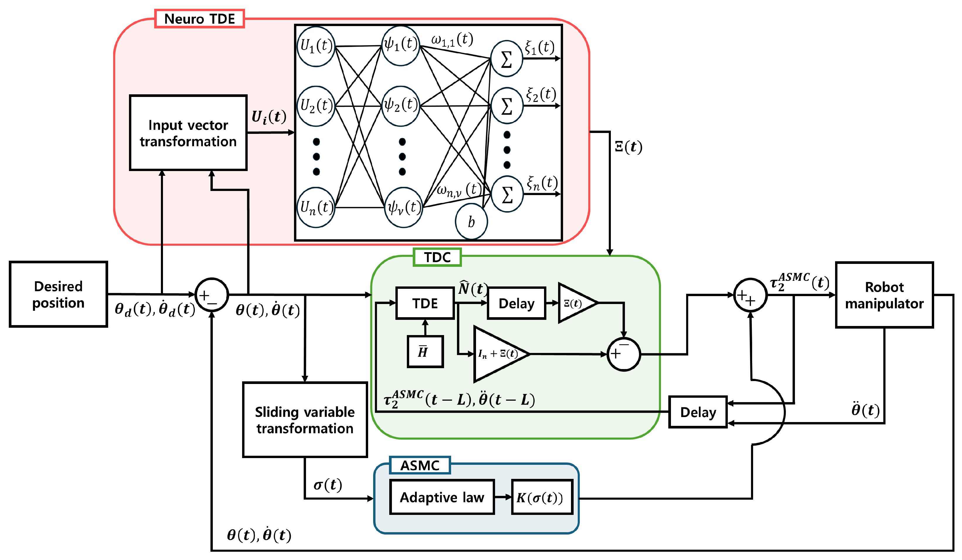
A quasi-convex function-based ASMC and a TDE enhanced by NNs are proposed in this paper, as illustrated in Figure 1. We have the following ASMC input.
When the ASMC (13) is utilized in place of the existing ASMC (12), the TDE error (11) transforms into the following TDE error:
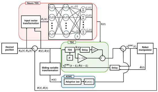
Figure 1.
Block diagram illustrating the structure of the proposed methods.
In this formulation, corresponds to the output of the proposed RBFNN, and . The proposed RBFNN architecture includes an input layer, a hidden layer with nonlinear activation functions, and an output layer. Its structure can be described as follows.
Here, denotes the number of hidden units. , , and b represent the weights, the input vector, and the bias, respectively, for and . The activation function is constructed using a Gaussian RBF, formulated as
where is defined as an input vector containing the tracking error, the desired position, and its velocity of the i-th joint. represents the squared Euclidean distance between the input vector and the center vector , given by . Here, is the center vector of the Gaussian RBF, and denotes its width parameter. The parameter determines the width of activation range of the basis function. A smaller results in a steeper variation of the function value near the center. The weight is updated using the following update law.
where and are positive scalars.
Remark 1.
Compared to the TDE in [8], which utilizes a fixed parameter α in (10), the TDE enhanced by NNs (13) utilizes tracking errors, desired positions, and their derivative as input data, enabling the estimation of for the current pose of robotic manipulators. Additionally, compared to those in [18,22], the proposed RBFNN incorporates a damping term in its weight update law (17) to prevent weight divergence. The effectiveness of the proposed TDE is shown through both simulation and experiment results.
The proposed function-based gain is defined as follows.
where and are positive tuning parameters. The parameter determines the overall scaling of the control gain. The parameter serves as a normalization factor that determines the degree to which the gain responds to the sliding variable. A smaller yields a steeper gain increase for small errors, while a larger results in a more gradual change. The gain function belongs to class in Definition 2 and satisfies the following properties:
- The is continuous on .
- The is at least with respect to on .
- The inverse function of exists.
- As approaches ∞, the approaches ∞.
Remark 2.
 Using the Lyapunov function (19), the main result can be formulated as follows.
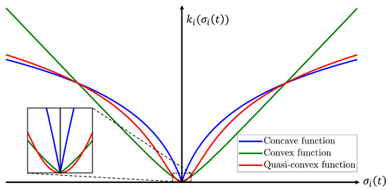
The continuous gain function (18) that is quasi-convex with respect to the magnitude of the sliding variable is proposed to replace the traditional switching control gain. The traditional switching-based adaptive law suffers from the drawback of inducing chattering phenomenon due to the discontinuous variation of the control gain. In contrast, the proposed function is a continuous function that belongs to class , allowing the control gain to be adjusted smoothly and continuously according to the magnitude of the sliding variable, thereby effectively mitigating this issue. Also, this function preserves smooth transitions between convex and concave characteristics depending on the magnitude of the sliding variable. As illustrated in Figure 2, a convex function has a steep gradient as the sliding variable increases, whereas a concave one has a steep gradient near the origin but becomes flatter as the sliding variable increases. Therefore, convex and concave function-based gains have drawbacks at large sliding variable values and near the origin, respectively. In contrast, the proposed quasi-convex function-based gain is convex near the origin and concave as the sliding variable increases. The effectiveness of the proposed function is verified via tracking performance and chattering phenomenon observed in the control torque.
Figure 2.
Comparison of class functions.
Theorem 1.
Proof.
The derivative of the Lyapunov function (19) with respect to time is computed as follows.
The derivative of the Lyapunov function (19) with respect to time is guaranteed to be negative if the gain function satisfies . Since is strictly increasing and belongs to class , its inverse also exists and belongs to the same class, as established in Lemma 1. Accordingly, one can define the threshold such that , which yields . Thus, if for each joint, the inequality holds, ensuring that . This result guarantees that converges to within the bound . □
Remark 3.
In the works [5,8], ASMC gain is updated according to the infinity norm of the sliding variable. Since such an adaptive law is mainly sensitive to the largest-magnitude element in the sliding variable or in the TDE error, there may exist conservative gain selection for the other joints except for the joint associated with the largest-magnitude element. In contrast, the proposed quasi-convex function-based gain tailored to individual joint behavior enables less conservative gain selection and individual bound (22) corresponding to each element of the sliding variable.
4. Simulation
4.1. Simulation Setup
The simulation is performed based on the dynamic model (2) of a 2-joint robotic manipulator, given by
where , and represents the joint position of i-th joint. The simulation model and parameters are adopted from [8] for consistency and comparability. In the system matrices (24), scalars are defined as [kg], [kg], [m], [m], and [m/s2]. The friction coefficients are [N· m · s], [N· m · s], [N· m · s], and [N· m · s]. The parameters used in the control torque are configured as [s], , , , and . The unpredictable disturbance is described by . The desired position is given by . We set the adjustable parameters of the RBFNN as , , , , , , , , , , , , , , , . The parameters of the quasi-convex function, and , are set to 10 and , respectively. For effective comparisons of control performance, this paper contains the results of the ASMC (12) using the convex function-based gain in [13], the proposed ASMC (13), and its specific case when . The parameters of the convex function-based gain, and , are set to 5 and , respectively.
4.2. Simulation Results
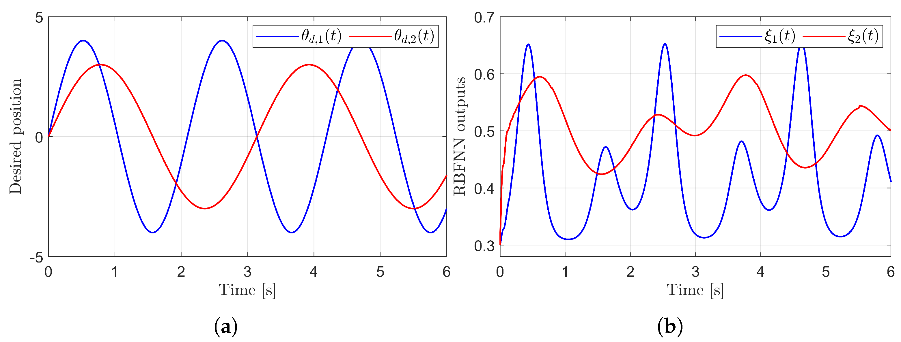
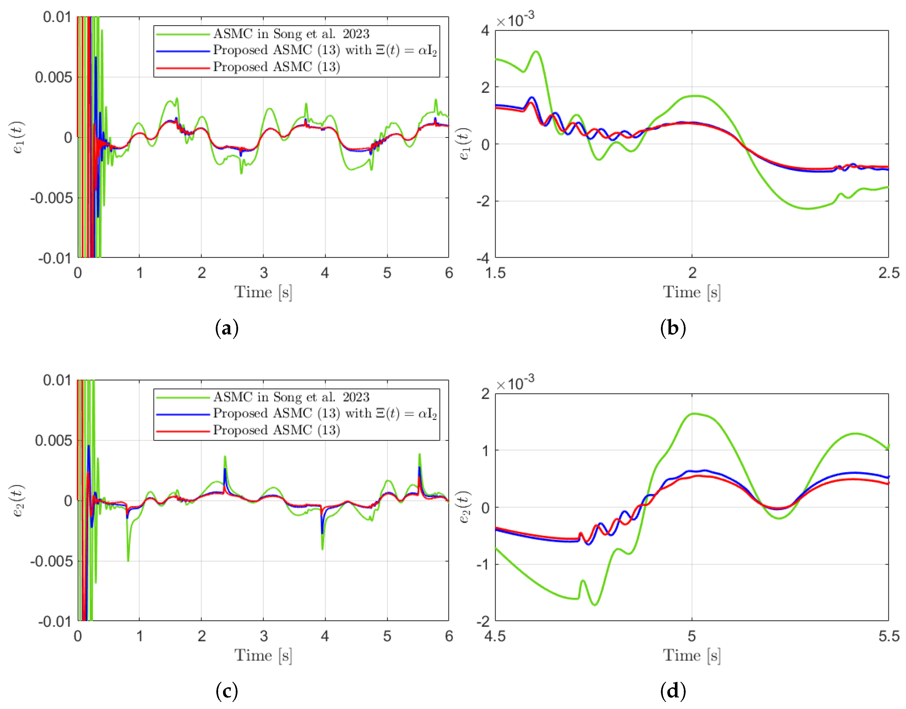
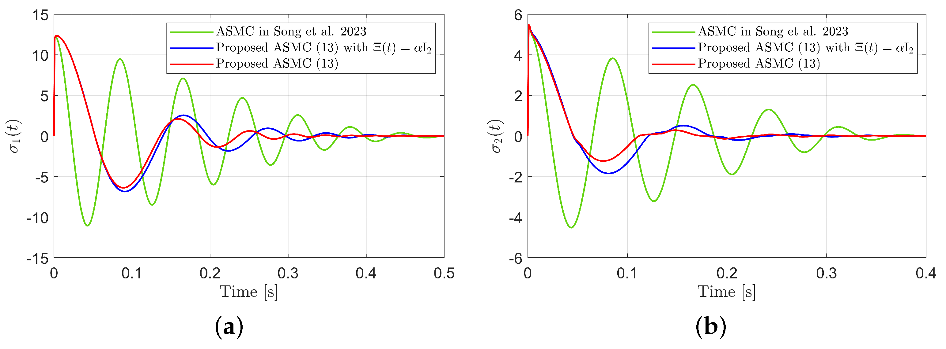
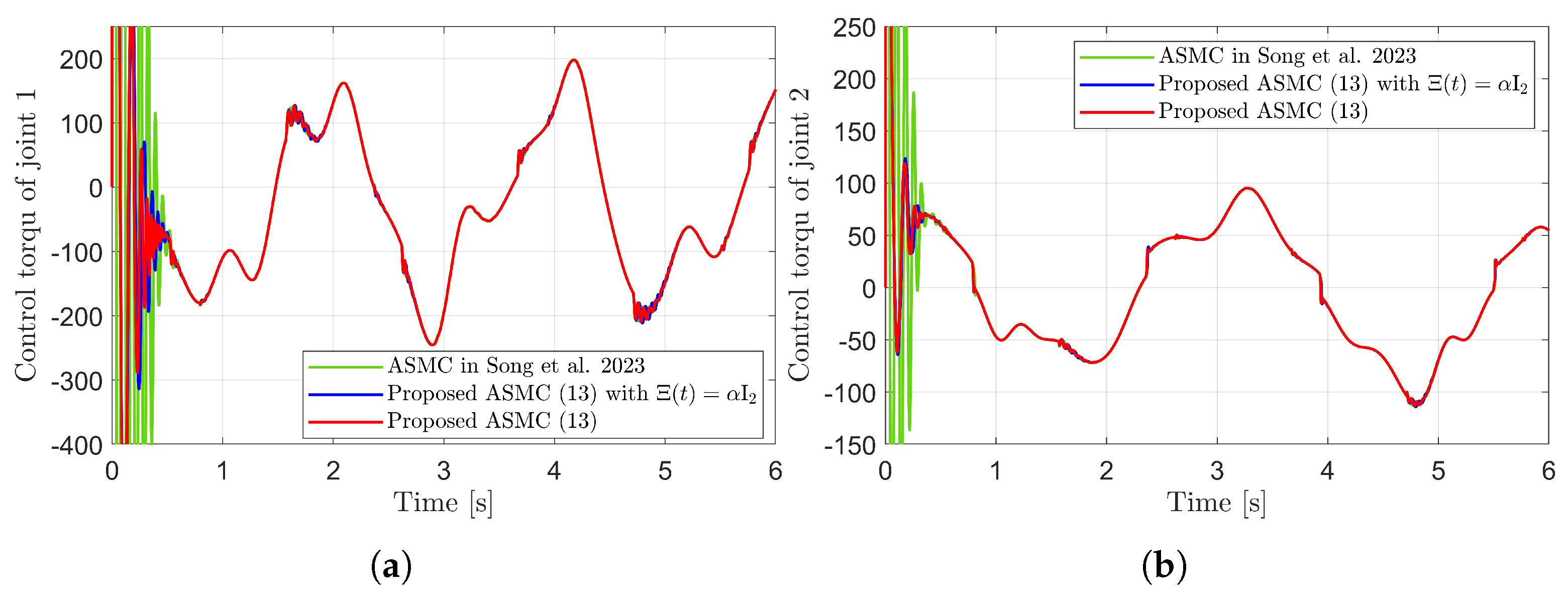
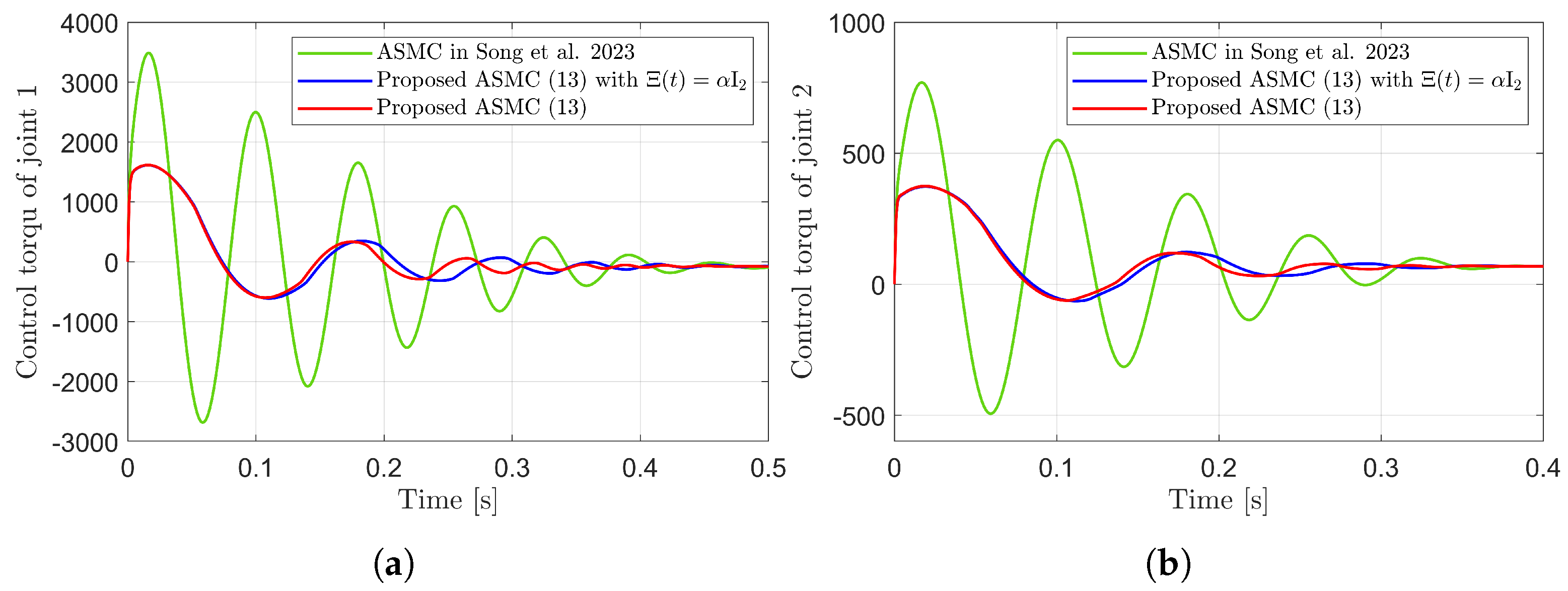
Figure 3 presents the desired position trajectories and associated RBFNN outputs which are elements of the estimated matrix . From Figure 3, it can be shown that the weight update law in (17) effectively prevents the RBFNN output from diverging. Figure 4 and Figure 5 illustrate that employing the estimated matrix significantly reduces tracking errors compared to the case using a constant parameter in the control input (13). In addition, Figure 4 and Figure 5 compare tracking performance of the proposed ASMC (13) when with the ASMC (12) using the convex function-based gain in [13]. Notably, Figure 6 reveals that the convex function-based ASMC induces more frequent oscillations during the reaching phase. Additionally, the rapid convergence of the sliding variable is not only essential for improving tracking accuracy and disturbance rejection, but also plays a critical role in ensuring reliable and real-time control in practical systems, as emphasized in [23,24]. The reduced chattering phenomenon in the proposed control torque is clearly observed in Figure 7 and Figure 8.
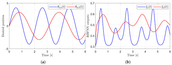
Figure 3.
Desired position trajectories and associated RBFNN outputs. (a) Desired positions. (b) RBFNN outputs.
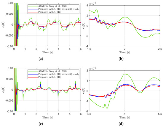
Figure 4.
Tracking errors and their enlarged views in the simulation compared with [13] (Song et al., 2023). (a) . (b) Enlarged view of . (c) . (d) Enlarged view of .
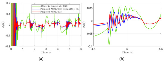
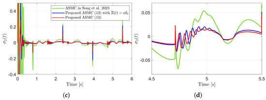
Figure 5.
Sliding variables and their enlarged views in the simulation compared with [13] (Song et al., 2023). (a) . (b) Enlarged view of . (c) . (d) Enlarged view of .
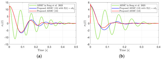
Figure 6.
Sliding variables during reaching phase in the simulation compared with [13] (Song et al., 2023). (a) . (b) .
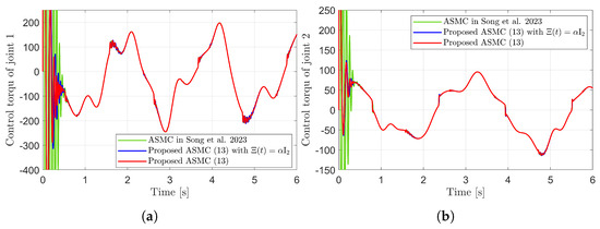
Figure 7.
Control torques in the simulation compared with [13] (Song et al., 2023). (a) Control torque of joint 1. (b) Control torque of joint 2.
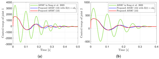
Figure 8.
Control torques during reaching phase in the simulation compared with [13] (Song et al., 2023). (a) Control torque of joint 1. (b) Control torque of joint 2.
5. Experiment
5.1. Experiment Setup
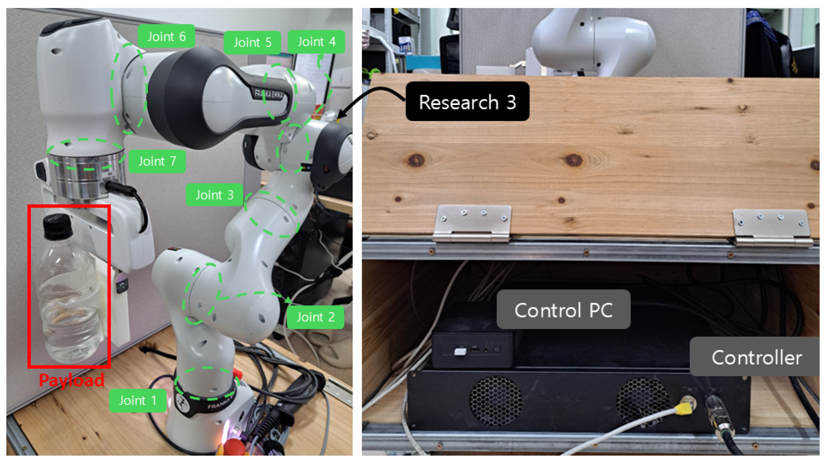
Figure 9 illustrates the 7-joint robotic manipulator, Franka Research 3, used in the experiment. The proposed controller was implemented using MATLAB/Simulink R2023b and executed on an Ubuntu 20.04 system. Real-time communication was established between MATLAB and the Franka Research 3 using the Franka Control Interface, enabling direct torque commands to be sent at each control cycle with a sampling rate of 1 kHz. Joint positions and velocities were measured using the internal encoders, while joint torques were obtained from the built-in torque sensors. The attached payload is 0.5 [kg], including the 0.338 [kg] weight of the water bottle. The attached payload generates highly irregular disturbances due to the movement of the water. Three control methods, referred as ASMC (12) using the convex function-based gain in [13], the proposed ASMC (13), and its specific case when , are compared in the experiment. The initial pose of Franka Research 3 is and the desired position is set as follows.
The center and the width of the RBFNN are chosen to be the same as those used in the simulation. The control parameters are set as follows. , , [s], , , , . The parameters of the quasi-convex function-based gain (18), and , are set to 10 and , respectively. The parameters of the convex function-based gain in [13], and , are set to 3 and , respectively.

Figure 9.
Franka Research 3 and control environments.
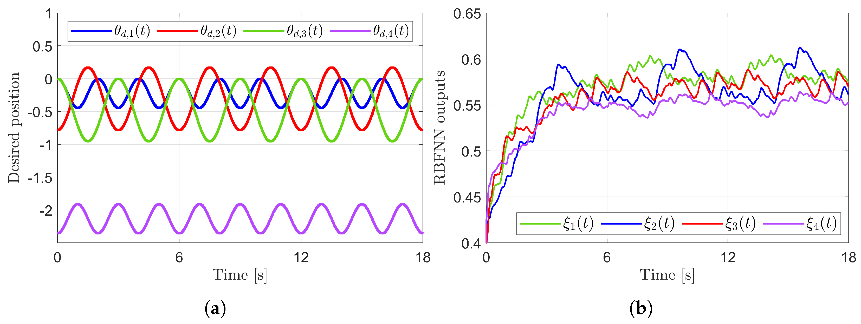
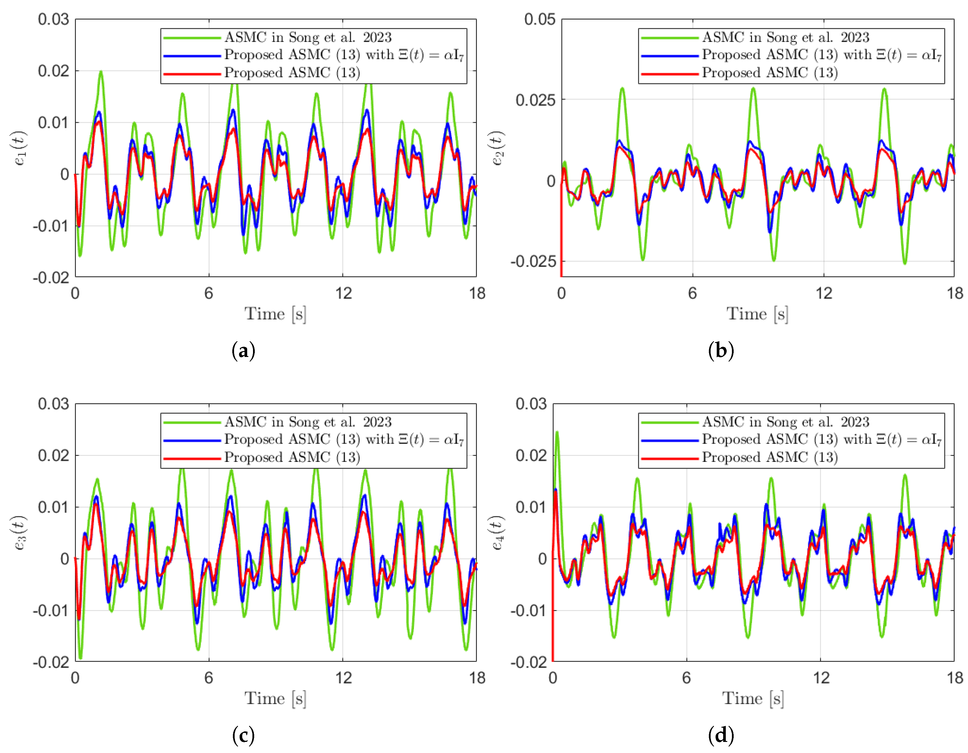
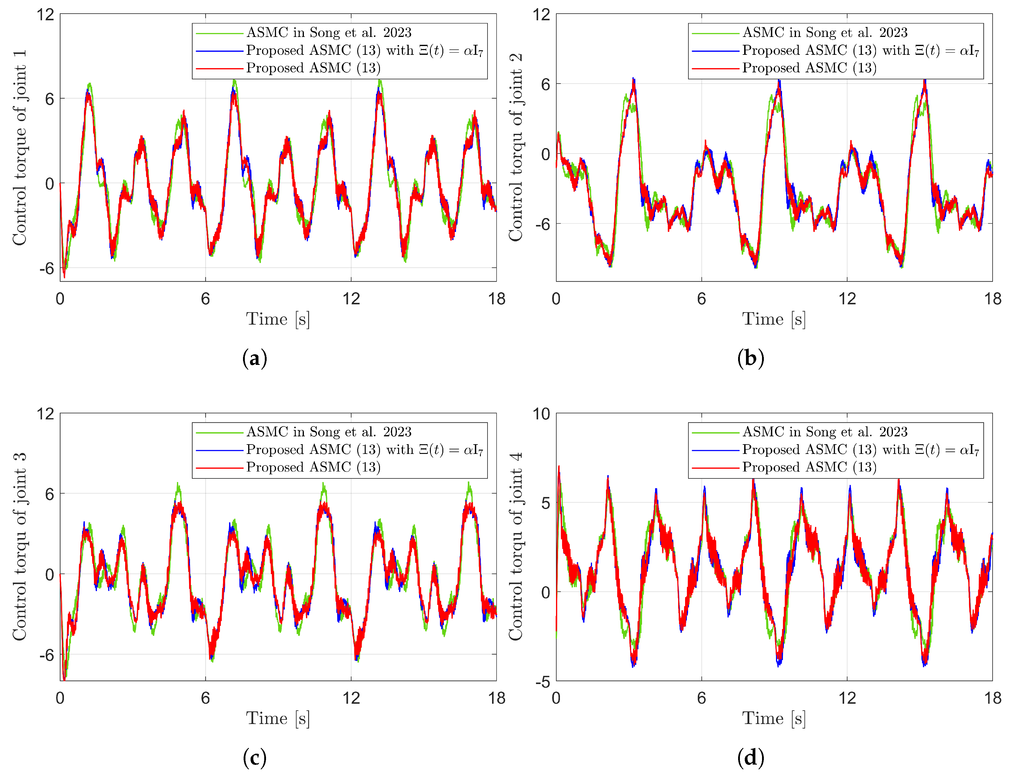
5.2. Experiment Results
Figure 10 presents the desired position trajectories along with the corresponding RBFNN outputs, which constitute the estimated matrix . It is observed that the weight update law in (17) effectively prevents the RBFNN output from diverging, even under real environments. Figure 11 and Figure 12 demonstrate that using the estimated leads to reduced tracking errors compared to the case using a fixed parameter in the control input (13). Furthermore, Figure 11 and Figure 12 compare the tracking performance of the proposed ASMC when with the ASMC (12) using the convex function-based gain in [13], showing that the proposed function contributes improved tracking performance. Notably, Figure 12 and Figure 13 reveal improved tracking performance with reduced chattering phenomenon of the proposed control torque (13).
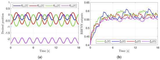
Figure 10.
Desired position trajectories and associated RBFNN outputs. (a) Desired position trajectories. (b) RBFNN outputs.
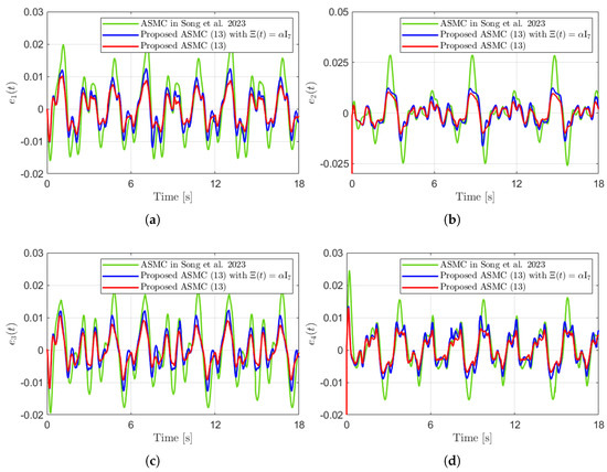
Figure 11.
Tracking errors in the experiment compared with [13] (Song et al., 2023). (a) . (b) . (c) . (d) .
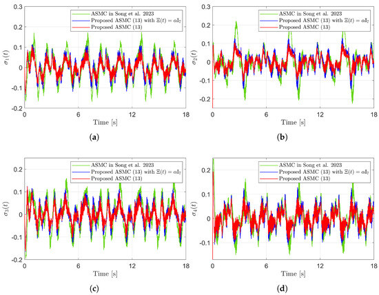
Figure 12.
Sliding variables in the experiment compared with [13] (Song et al., 2023). (a) . (b) . (c) . (d) .
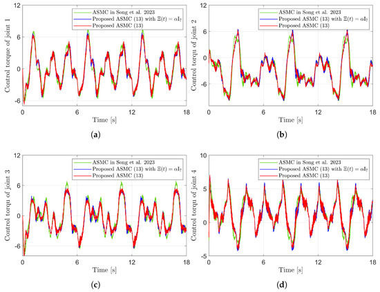
Figure 13.
Comparison of control torques in the experiment compared with [13] (Song et al., 2023). (a) Control torque of joint 1. (b) Control torque of joint 2. (c) Control torque of joint 3. (d) Control torque of joint 4.
Remark 4.
In addition to the simulation, the effectiveness of the proposed control method is verified through an experiment using a real 7-joint robotic manipulator, Franka Research 3. The proposed control method is tested with highly irregular disturbances caused by a water-filled payload during fast motion. The results demonstrate that the proposed control method is not only theoretically sound but also practical and robust for robotic manipulator applications in real environments.
6. Conclusions
This paper proposed the ASMC strategy tailored for robotic manipulators, featuring a quasi-convex function-based control gain and the TDE enhanced by NNs. To compensate for TDE errors, the proposed method utilized both the previous TDE error and the RBFNN with a weight update law that includes a damping term to prevent divergence. Additionally, a continuous gain that is quasi-convex function is proposed to replace the traditional switching control gain. This function preserved the continuous gain and smooth transitions between convex and concave characteristics depending on the magnitude of the sliding variable. As a result, the proposed gain effectively suppressed the chattering phenomenon caused by abrupt changes in the SMC gain and mitigated the overestimation problem associated with the convex function. The stability of the proposed control method is guaranteed in the sense of uniform ultimate boundedness, and its effectiveness was validated through both simulation and experiment results. In future work, the proposed ASMC method will be extended to complex robot systems.
Author Contributions
Conceptualization, J.W.L.; Funding acquisition, S.Y.L.; Investigation, J.W.L., J.M.R., S.G.P. and H.M.A.; Project administration, S.Y.L.; Supervision, M.K. and S.Y.L.; Validation, H.M.A.; Visualization, J.M.R. and S.G.P.; Writing—original draft, J.W.L. and S.Y.L.; Writing—review and editing, M.K. and S.Y.L. All authors have read and agreed to the published version of the manuscript.
Funding
This work was supported by the Soonchunhyang University Research Fund. This work was supported by the faculty research fund of Sejong University in 2025.
Institutional Review Board Statement
Not applicable.
Informed Consent Statement
Not applicable.
Data Availability Statement
Data are contained within the article.
Conflicts of Interest
The authors declare no conflicts of interest.
References
- Yang, M.; Yu, L.; Wong, C.; Mineo, C.; Yang, E.; Bomphray, I.; Huang, R. A cooperative mobile robot and manipulator system (Co-MRMS) for transport and lay-up of fibre plies in modern composite material manufacture. Int. J. Adv. Manuf. Technol. 2022, 119, 1249–1265. [Google Scholar] [CrossRef]
- Li, C.; Yan, Y.; Xiao, X.; Gu, X.; Gao, H.; Duan, X.; Zuo, X.; Li, Y.; Ren, H. A Miniature Manipulator with Variable Stiffness Towards Minimally Invasive Transluminal Endoscopic Surgery. IEEE Robot. Autom. Lett. 2021, 6, 5541–5548. [Google Scholar] [CrossRef]
- Ghodsian, N.; Benfriha, K.; Olabi, A.; Gopinath, V.; Arnou, A. Mobile Manipulators in Industry 4.0: A Review of Developments for Industrial Applications. Sensors 2023, 23, 8026. [Google Scholar] [CrossRef] [PubMed]
- Mandil, W.; Rajendran, V.; Nazari, K.; Ghalamzan-Esfahani, A. Tactile-Sensing Technologies: Trends, Challenges and Outlook in Agri-Food Manipulation. Sensors 2023, 23, 7362. [Google Scholar] [CrossRef] [PubMed]
- Baek, J.; Jin, M.; Han, S. A New Adaptive Sliding-Mode Control Scheme for Application to Robot Manipulators. IEEE Trans. Ind. Electron. 2016, 63, 3628–3637. [Google Scholar] [CrossRef]
- Jin, M.; Kang, S.H.; Chang, P.H.; Lee, J. Robust Control of Robot Manipulators Using Inclusive and Enhanced Time Delay Control. IEEE/ASME Trans. Mechatronics 2017, 22, 2141–2152. [Google Scholar] [CrossRef]
- Lee, J.; Chang, P.H.; Seo, K.H.; Jin, M. Stable Gain Adaptation for Time-Delay Control of Robot Manipulators. IFAC-PapersOnLine 2019, 52, 217–222. [Google Scholar] [CrossRef]
- Park, J.; Kwon, W.; Park, P. An Improved Adaptive Sliding Mode Control Based on Time-Delay Control for Robot Manipulators. IEEE Trans. Ind. Electron. 2023, 70, 10363–10373. [Google Scholar] [CrossRef]
- Young, K.; Utkin, V.; Ozguner, U. A control engineer’s guide to sliding mode control. IEEE Trans. Control Syst. Technol. 1999, 7, 328–342. [Google Scholar] [CrossRef]
- Utkin, V.; Guldner, J.; Shi, J. Sliding Mode Control in Electro-Mechanical Systems; CRC Press: Boca Raton, FL, USA, 2017. [Google Scholar]
- Utkin, V.I.; Poznyak, A.S. Adaptive sliding mode control. In Advances in Sliding Mode Control: Concept, Theory and Implementation; Springer: Berlin/Heidelberg, Germany, 2013; pp. 21–53. [Google Scholar]
- Obeid, H.; Fridman, L.M.; Laghrouche, S.; Harmouche, M. Barrier Function-Based Adaptive Sliding Mode Control. Automatica 2018, 93, 540–544. [Google Scholar] [CrossRef]
- Song, J.; Zuo, Z.; Basin, M. New Class K∞ Function-Based Adaptive Sliding Mode Control. IEEE Trans. Autom. Control 2023, 68, 7840–7847. [Google Scholar] [CrossRef]
- Feng, H.; Song, Q.; Ma, S.; Ma, W.; Yin, C.; Cao, D.; Yu, H. A new adaptive sliding mode controller based on the RBF neural network for an electro-hydraulic servo system. ISA Trans. 2022, 129, 472–484. [Google Scholar] [CrossRef] [PubMed]
- Fei, J.; Wang, Z.; Pan, Q. Self-Constructing Fuzzy Neural Fractional-Order Sliding Mode Control of Active Power Filter. IEEE Trans. Neural Netw. Learn. Syst. 2023, 34, 10600–10611. [Google Scholar] [CrossRef] [PubMed]
- Fei, J.; Ding, H. Adaptive sliding mode control of dynamic system using RBF neural network. Nonlinear Dyn. 2012, 70, 1563–1573. [Google Scholar] [CrossRef]
- Hu, J.; Zhang, D.; Wu, Z.G.; Li, H. Neural network-based adaptive second-order sliding mode control for uncertain manipulator systems with input saturation. ISA Trans. 2023, 136, 126–138. [Google Scholar] [CrossRef] [PubMed]
- Zhang, X.; Wang, H.; Tian, Y.; Peyrodie, L.; Wang, X. Model-free based neural network control with time-delay estimation for lower extremity exoskeleton. Neurocomputing 2018, 272, 178–188. [Google Scholar] [CrossRef]
- Han, S.; Wang, H.; Tian, Y.; Christov, N. Time-delay estimation based computed torque control with robust adaptive RBF neural network compensator for a rehabilitation exoskeleton. ISA Trans. 2020, 97, 171–181. [Google Scholar] [CrossRef] [PubMed]
- Utkin, V.I. Sliding Modes in Control and Optimization; Communications and Control Engineering Series; Springer: Berlin/Heidelberg, Germany, 1992. [Google Scholar]
- Khalil, H.K.; Grizzle, J.W. Nonlinear Systems; Prentice Hall: Upper Saddle River, NJ, USA, 2002; Volume 3. [Google Scholar]
- Su, J.; Wang, L.; Liu, C.; Qiao, H. Robotic Inserting a Moving Object Using Visual-Based Control with Time-Delay Compensator. IEEE Trans. Ind. Inform. 2024, 20, 1842–1852. [Google Scholar] [CrossRef]
- Xu, H.; Yu, D.; Wang, Z.; Cheong, K.H.; Chen, C.L.P. Nonsingular Predefined Time Adaptive Dynamic Surface Control for Quantized Nonlinear Systems. IEEE Trans. Syst. Man Cybern. Syst. 2024, 54, 5567–5579. [Google Scholar] [CrossRef]
- Yang, Y.; Sui, S.; Liu, T.; Philip Chen, C.L. Adaptive Predefined Time Control for Stochastic Switched Nonlinear Systems with Full-State Error Constraints and Input Quantization. IEEE Trans. Cybern. 2025, 55, 2261–2272. [Google Scholar] [CrossRef] [PubMed]


Disclaimer/Publisher’s Note: The statements, opinions and data contained in all publications are solely those of the individual author(s) and contributor(s) and not of MDPI and/or the editor(s). MDPI and/or the editor(s) disclaim responsibility for any injury to people or property resulting from any ideas, methods, instructions or products referred to in the content. |
© 2025 by the authors. Licensee MDPI, Basel, Switzerland. This article is an open access article distributed under the terms and conditions of the Creative Commons Attribution (CC BY) license (https://creativecommons.org/licenses/by/4.0/).