Article

New Possibilities of Field Data Survey in Forest Road Design

1
Department of Forest Engineering, Faculty of Forestry and Wood Technology, University of Zagreb, Svetošimunska Cesta 23, 10 000 Zagreb, Croatia
2
Croatian Forests Ltd., Forest Administration Office Delnice, Supilova 32, 51300 Delnice, Croatia
*
Author to whom correspondence should be addressed.
Sensors 2025, 25(13), 4192; https://doi.org/10.3390/s25134192 (registering DOI)
Submission received: 21 May 2025 / Revised: 20 June 2025 / Accepted: 23 June 2025 / Published: 5 July 2025
(This article belongs to the Special Issue Application of LiDAR Remote Sensing and Mapping)

Abstract

Field data, as the basis for planning and designing forest roads, must have high spatial accuracy. Classical (using a theodolite and a level) and modern (based on total stations and GNSSs) surveying methods are used in current field data survey for forest road design. This study analyzed the spatial accuracy of classical and modern surveying methods, the accuracy of spatial data recorded using a UAV equipped with an RGB camera at different flight altitudes, and the accuracy of lidar data of the Republic of Croatia. This study was conducted on a forest area where salvage logging was carried out, which enabled the use of a GNSS receiver in RTK mode as a reference method. The highest RMSE values of the spatial coordinates were recorded for measurements obtained with the classical surveying method (0.89 m) and a total station (0.33 m). The flight altitude of the UAV did not significantly affect the spatial error of the collected data, which ranged between 0.07 and 0.09 m. The cross-terrain slope, as one of the factors that significantly affect the amount of earthworks, did not differ statistically significantly between the methods. The ALS error was strongly influenced by the cross-terrain slope. The authors conclude that the new survey methods (SfM and lidar data) provide high-accuracy data but also draw attention to challenges in their use, such as vegetation and biomass on the ground.

1. Introduction

The establishment of an optimal forest road network requires four phases: the planning, design, construction, and management of forest roads [1]. The absence or poor performance of any of the mentioned phases consequently causes various negative impacts on the forest road, the area in which the forest road is located, and the costs of harvesting [2,3,4,5,6]. The forest road design phase can be divided into two separate but mutually dependent subphases: subphase 1 refers to the collection of general and technical data, and subphase 2 is divided into (2a) field surveys and (2b) project development, i.e., office data processing, printing, and results drawing [7]. The office processing of the collected data is carried out with the help of specialized software packages for the design of forest roads, such as RoadEng (Softree Technical Systems). In addition to specialized programs, to design forest roads, programs developed for the design of public roads, such as the Civil 3D software, can also be used. Regardless of the program used, field data, which are the basis for planning and designing a forest road, must be of high spatial accuracy [8]. For field data collection, to design forest roads, various methods of measurement are used in forestry [9]:
  • The classical method (using theodolites, levels, and inclinometers);
  • The modern method (based on total stations and GNSSs).
The classic method of measurement involves the use of a theodolite, a level, and an inclinometer. The theodolite is the most precise instrument designed for the measurement of horizontal and vertical angles [10]. The total station was developed by combining the angle-measuring capabilities of a theodolite with an electronic distance measurement (EDM) [11]. A total station can determine the horizontal angle, vertical angle, and slope distance to a particular point. A total station, similar to a theodolite, achieves extremely high horizontal and vertical accuracy, with an error of 0.00028–0.00139 degrees [12]. The accuracy of these almost perfect measuring devices can be influenced by factors such as human error (collimation and pointing errors) [13,14] or the calibration and malfunction of the device (optical plummet errors, atmospheric corrections, and the adjustment of the prism poles error) [14]. As the work with the theodolite and the total station is time-consuming [11,15,16], and the lack of labor in forestry and construction is a growing problem [17,18,19], it should not be surprising that GNSS receivers are being implemented in forestry [20,21]. GNSS surveys using a GNSS receiver in real-time kinematics mode (RTK) can achieve subcentimeter accuracy [16,22,23]. Several factors can affect GNSS accuracy: (1) the canopy structure and its density; (2) the tree type; (3) the terrain area; and (4) the field measurement season [24,25,26]. In addition to these measuring devices, data obtained via a photogrammetric analysis or recorded with lidar sensors have been increasingly used in recent times. These methods, as a new way of measuring, could be classified as experimental methods of measurement. The implementation of UAVs in forestry, equipped with sensors for photogrammetric and lidar imaging, is well accepted, primarily due to their autonomy, reliability, safety, and control [27]. Although in certain professions and forestry works, these experimental methods represent “go-to” methods for measurement [28,29,30,31,32], their accuracy needs to be tested for forest road planning and design.
In previous studies on the spatial accuracy of photogrammetric data recorded with UAVs (UAV SfM), the recorded root-mean-square error (RMSE) ranged between 2.3 and 123 cm [33,34,35,36,37,38]. The accuracy of this system can be influenced by several factors, such as flight parameters [39], georeferencing and correction methods [34,36], and lighting [40]. Lepoglavec et al. [41] found no significant differences in the longitudinal slope of the road between a GNSS and the digital terrain model (DTM) developed based on UAV aerial photographs. Depending on the method used to collect lidar data and the sensors themselves, the RMSE of the spatial data can range from 7 cm, for data collected with UAVs, equipped with a lidar sensor [42], and between 12 and 50 cm for data collected with lidar sensors, installed on aircraft [43,44,45]. Kweon et al. [46] determined that the error in the recorded length of measured forest roads with a mobile laser scanner (MLS), compared with a GNSS, ranged from 0.1 to 0.7 m, while the difference between the GNSS and a total station was 2.1 to 4.7 m.
This research tested the spatial accuracy of data recorded using different measurement methods—the classical method; the modern method; the use of an unmanned aerial vehicle equipped with an RGB camera at different flight altitudes; and lidar data, based on airborne laser scanning (ALS)—to collect data necessary for the design of forest roads. Furthermore, as the cross-terrain slope can significantly affect earthwork volumes [47], which, consequently, affect the cost of forest road construction [48], the differences in the obtained cross-terrain slopes were also examined. Finally, the differences in the forest road planned route central axis, measured using different field survey methods, (theodolites, total stations, GNSSs, and UAVs) were tested.

2. Materials and Methods
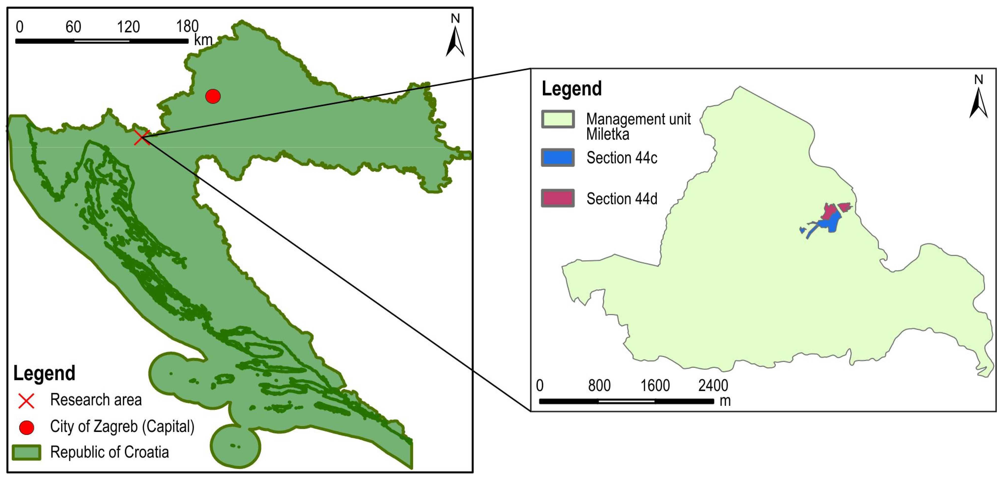
2.1. Research Area

This research was conducted in the state forests of the Republic of Croatia managed by the company Croatian Forests Ltd., Forest Administration Delnice, Forest office Vrbovsko, Management Unit Miletka, Sections 44 c and 44 d (Figure 1). The phytocenose of the above forest sections is Aremonio-Piceetum (Horvat 1938), where common spruce (Picea abies L.) predominates. According to the Mellgren classification [49], the investigated area has a moderately steep terrain (32%). In 2017, salvage logging was carried out in the investigated sections due to attacks from bark beetle (Ips typographus L.). After felling, the forest order was established, and for this reason, a large amount of biomass (in heaps) was left on the ground (Figure 2B). As only individual trees were present in the study area, more than 90% of the area was not under tree canopy.

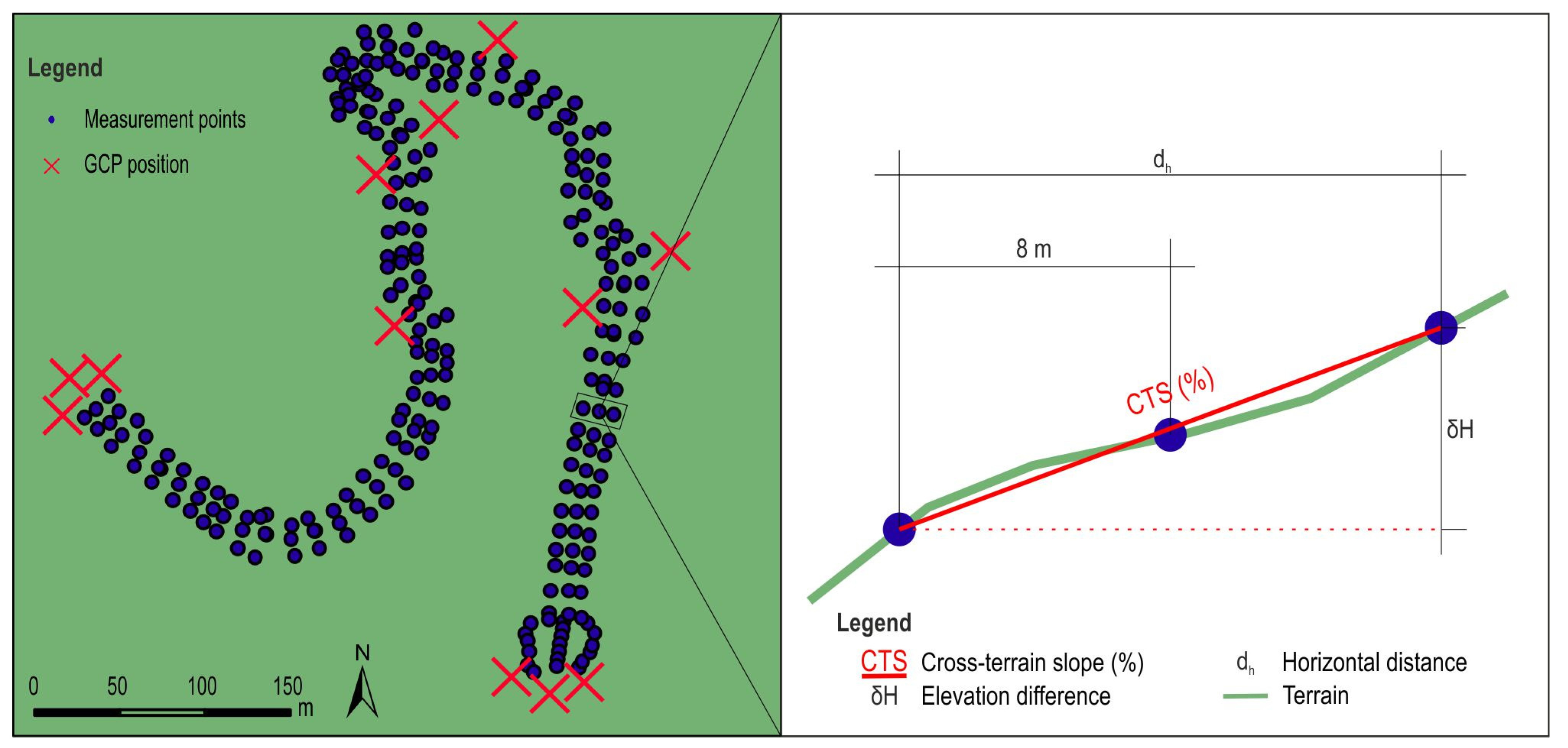
2.2. Data Collection

Data collection was carried out using a classical, modern and experimental method of survey. Before the start of the field survey, a zero line was planned on the contour map at M 1:25,000. The maximum longitudinal slope of the used zero line did not exceed 10%, which is fully in accordance with the technical specifications of forest roads in the Republic of Croatia [50,51]. This was followed by the transfer of the planned zero line to the terrain and the fitting of the horizontal alignment polygon, which ultimately represented the final horizontal central axis of the planned forest road. The zero line was placed and the horizontal alignment was decided according to the methods described by Pičman [52]. The set polygon consisted of 30 intersection points (IPs) with a total length of 879.42 m.

2.2.1. Classical Method of Measurement

For this study, a theodolite, a level, and a measuring rod were used as the classical method of survey. The classical survey method was included in this study as it is still used in specific forest conditions such as dense forest areas, where the use of a total station and its EDM can be very limited with a lack of prism (reflector) sight. After placing the horizontal alignment polygon, the deflection angles were measured with a digital theodolite (Geomax ZIPP 02) (Figure 3A), the radii were defined, and the main elements of each horizontal curve were calculated based on these values. This was followed by staking out the horizontal curves, which defined the positions of the beginning, middle, and end of the curve of each horizontal curve, while on the flat parts of the route, where the distance between the end of the curve of the previous horizontal curve and the beginning of the curve of the next horizontal curve was more than 15 m, additional profiles were placed (intermediate points). In this case, the distance of the intermediate point from the previous profile was 10 m. Based on 30 intersection points (IPs), a total of 28 horizontal curves were staked, which also represented the number of times the instrument was moved (Figure 3A). A total of 98 profiles (start, middle, and end points of the horizontal curves and intermediate points) were placed on the planned route of the forest road. The positions of the beginning and end of the arc (horizontal curve) were determined based on the following formula (1) for calculating the tangent value:
T g = R × t g α 2
where
Tg—tangent value (m);
R—selected radius (m);
α—deflection angle (°).
Figure 3. Principles of operation for each measuring device: (A) theodolite, (B) total station, (C) GNSS, and (D) UAV SfM.
Sensors 25 04192 g003
The leveling of the profiles was carried out using a level (Sokkia C330) and a geodetic rod. When leveling the profile, the device was moved 28 times. Terrain cross sections were recorded using two geodetic rods, recording the relative relationships (increase or decrease in the elevation) every two meters perpendicular to the position of the profile with an accuracy of 1 mm. This way, the cross section of the terrain was recorded in a strip of 16 m around the central axis of the planned forest road. The survey with the theodolite and level required two people, while the recording of the terrain cross section required three people.

2.2.2. Modern Method of Measurement

For the modern field survey method, the Stonex R35 total station (Figure 3B) and the Stonex S900A GNSS (Figure 3C) were used. All the profiles placed on the horizontal polygon of the planned forest road and the terrain cross section were recorded at the same points where classic survey method points were recorded. In each profile, three terrain points were recorded with a total station and a GNSS receiver: one on the central axis of the planned forest road route and one each perpendicular to the central axis at a distance of 8 m to the left and right (Figure 4). A total of 250 points were recorded with these devices. In places where certain profiles were almost in the same position (connected horizontal curves in the same or different directions), the points on the central axis were recorded, indicating the position of the profile, and the end of the 8 m band was recorded with one point for both profiles. The total station was moved a total of 28 times. The GNSS was used in RTK mode. The used correction base was the Croatian Positioning System (CROPOS). CROPOS is a system of 59 reference GNSS stations located 70 km from each other. Reference stations collect satellite measurement data and calculate correction parameters available to field users via mobile Internet (GPRS/GSM) [53]. A total station field survey requires two people, while only one is needed for a GNSS receiver survey.

2.2.3. Experimental Method of Measurement

The research area was recorded using a UAV (DJI Mavic 3 Enterprise) (Figure 3D). The flight mission was created in DJI Pilot 2. Four surveys were performed:
  • At a height of 60 m with the terrain follow function disabled (60NF);
  • At a height of 70 m with the terrain follow function disabled (70NF);
  • At a height of 70 m with terrain follow function enabled (70F);
  • At a height of 90 m with terrain follow function enabled (90F).
Flying at an altitude of 60 m using the terrain follow option was not possible due to the power line located at the research site. The terrain follow option cannot be turned off when flying at an altitude of 90 m because the flying height in certain parts of the research area would then be higher than 120 m above the ground, which violates the legislation on UAV use in the Republic of Croatia. In all four flight missions, 80% front and 80% side overlaps of aerophotographs were used. During flights, the UAV was equipped with an RTK module, and additional ground control points (GCPs) were placed on the ground (12). GCPs were recorded with a GNSS receiver according to the method followed in Mihelič et al. [54]. Check point markings (a cross on A4 paper), used to analyze the spatial accuracy of the data collected with the UAV, were placed at the same positions where the terrain points were recorded with the classic and modern survey methods.
In addition to UAV surveys, as an experimental survey method, ALS data from the Croatian Geodetic Administration was also tested. ALS data was used in the part of the analyses that required no ground markings. According to the lidar product specification, in areas covered with forests (deciduous and coniferous), the minimum required point density was 4 points/m2, with a minimum height accuracy of ±0.1 m (z coordinates) and a horizontal accuracy of ±0.2 m (xy coordinates) [55]. Based on the lidar data, a DTM with a grid width of 1 m (1 × 1 m) (DTMALS) was created. The point elevations (z coordinates) of the created DTM of the planned forest road were extracted in ArcMap (v. 10.8) using the Add Surface Information tool. The points recorded by a GNSS receiver were used as positions for z-coordinate extraction.

2.3. Data Processing

Classical survey method recordings were entered into the Cesta (v 1.6) software. On the basis of the azimuths, profile heights, and terrain cross-section development, spatial data was obtained. The first and second theodolite survey points were georeferenced based on a GNSS survey.
A photogrammetric analysis of the collected UAV aerial photographs (UAV SfM) was performed in the Pix4D mapper software (v 4.8.4) (Table 1). Based on the results of the analysis, digital terrain models (DTMs) were developed for each flight:
  • 60NF digital terrain model (DTM60NF);
  • 70NF digital terrain model (DTM70NF);
  • 70F digital terrain model (DTM70F);
  • 90F digital terrain model (DTM90F).
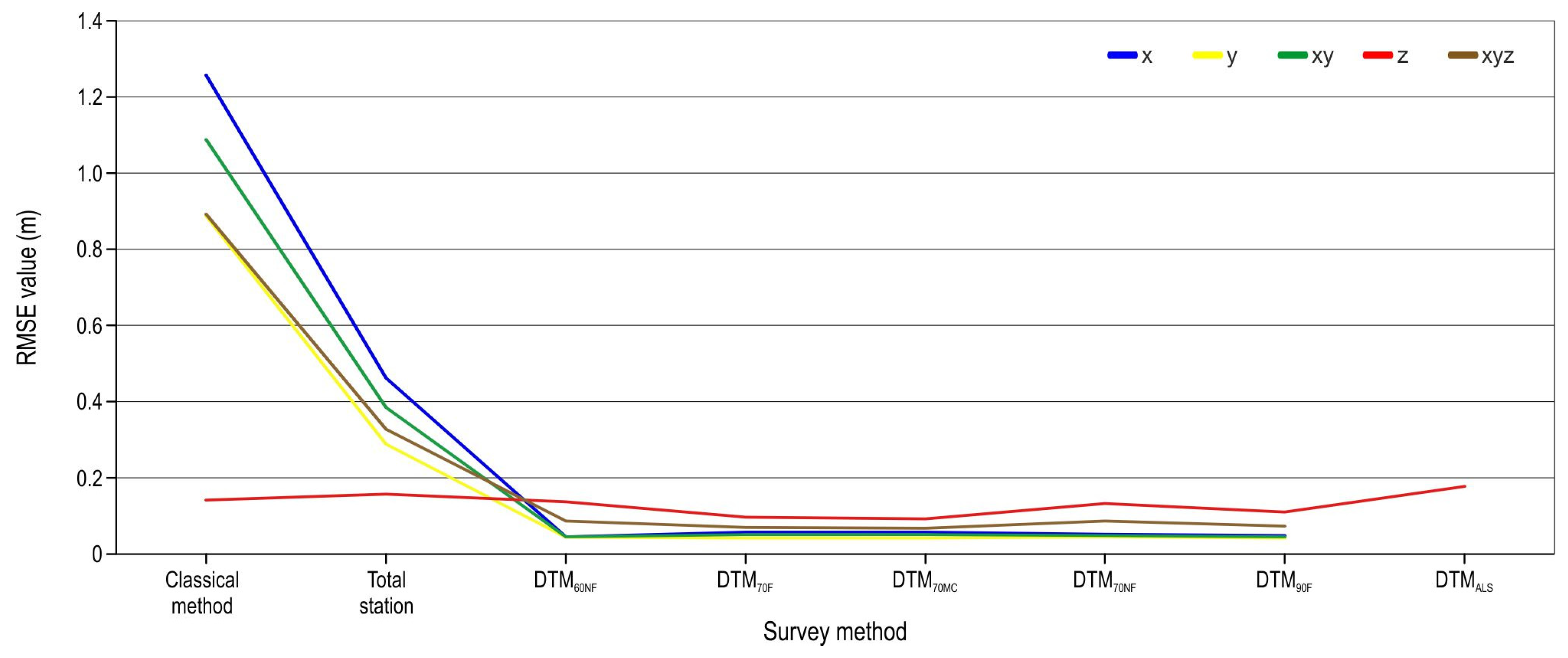
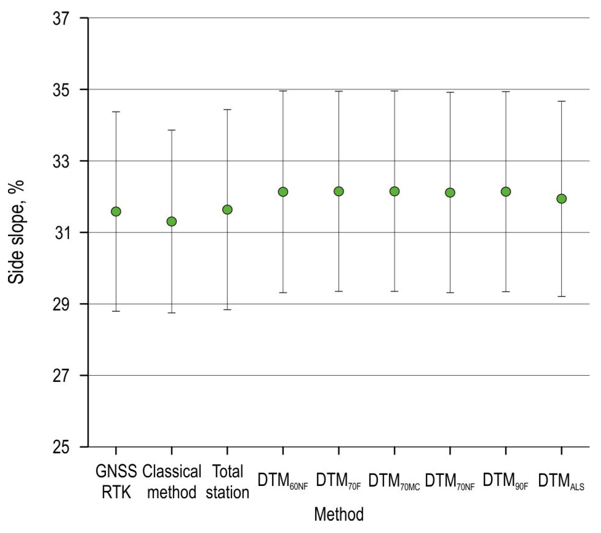
The Pix4D mapper software offers automatic point cloud classification. Due to the larger amount of biomass on the ground during this study (established forest order), it was noticed that, in some places, points were classified as ground, which was not true in reality. This software uses only points classified as ground or road for the development of a DTM. Since such places, in the case of insufficiently good classification, can cause possible errors, additional manual classification of point clouds was performed, based on 70F, and a new DTM (DTM70MC) was created. The time required for the manual classification of the point cloud was 7 h.
In further analysis, the GNSS survey was used as a reference measurement method.
A database was created in MS Excel, and the RMSE of spatial coordinates (x, y, xy, z, and xyz) of the terrain points was calculated according to the following Formula (2):
R M S E c o o r d i n a t e d = c o o r d i n a t e d 2 n
where
c o o r d i n a t e d —spatial difference (x, y, xy, z, or xyz);
n—number of terrain points.
For an analysis of spatial coordinates’ RMSE, the same measurement points (their placement) for each survey method were used.
Next, the analysis of spatial coordinates’ error dependence on station (distance from the first profile) was conducted.
In addition to the RMSE of spatial coordinates, the recorded average cross-terrain slope for each profile was also analyzed (Figure 4). The average cross-terrain slope was calculated according to the following Formula (3):
C T S = δ H d h
where
CTS—cross-terrain slope (%);
δH—height difference (z);
d h —horizontal distance between cross-section end points.
Finally, the deviation of the recorded points of the central axis was analyzed via the method used in the study by Kweon et al. [46]. The centerline points recorded by the theodolite, total station, and UAV SfM surveys were overlaid with the buffer zone around the GNSS centerline. The radius of the buffer zone was increased by 0.1 m until 100% of all survey points were inside it.
A statistical analysis was performed in IBM SPSS Statistics (v.29.0). Data normality testing was performed using a Kolmogorov–Smirnov test. One-way analysis of variance (ANOVA) followed by the Tukey post hoc test was used to determine the differences between terrain side slopes measured with the tested methods. A correlation and regression analysis was used to determine the relationship and connection between the cross-terrain slope and measurement error.

3. Results

The central axis of the planned forest road route recorded with the GNSS receiver was 879.42 m. The total station survey was the only method with a shorter recorded centerline (879.39 m). The difference in the central axis length recorded via the UAV SfM survey differed between +0.02 m (DTM60NF) and +0.13 m (DTM70NF). The height difference between the first and last points of the central axis measured with the GNSS receiver was 66.50 m. All UAV SfM surveys recorded smaller elevation differences between the first and last points. The classical survey method (level) and total station recorded higher elevation differences and greater longitudinal slopes versus the GNSS survey (Table 2).
The spatial accuracy of the recorded points (x, y, and z value) was tested on 250 points (Table 3). The largest spatial deviation (of all coordinates) was recorded for the classic survey method—using a theodolite and a level. All survey methods recorded higher RMSE values for the x-axis versus the y-axis. The UAV SfM DTM spatial errors were approximately the same (0.19–0.22 m). With manual classification of the point clouds, the z-coordinate RMSE value of DTM70MC was reduced by 0.01 m compared with that of DTM70F.
The program used for classical survey method field data processing (Cesta) places cross-terrain points perpendicular to the central axis (points) of the road. Although special care was taken to record the cross-terrain points perpendicular to the central axis, certain deviations were found that affected the results of the analysis. For this reason, a spatial analysis of only the points that represented the central axis of the planned forest road (98 points) was carried out. The new analysis showed lower RMSE values for all survey methods (Figure 5). The classical survey method recorded the highest RMSE value for both the x (1.25 m) and y (0.89 m) coordinates. On the other hand, the smallest horizontal coordinate RMSE values were recorded for the UAV SfM survey: DTM60NF (0.04 m) for the x coordinate and DTM70F (0.04 m) for the y coordinate. The highest recorded z-coordinate RMSE values were calculated for DTMALS (0.18 m) and total station (0.16 m). The Z value RMSE of the UAV SfM survey ranged between 0.09 m (DTM70MC) and 0.14 m (DTM60NF). With manual classification of the point cloud (DTM70MC), the z-coordinate RMSE value was reduced by 0.01 m compared with that for the automatic classification of the same point cloud (DTM70F–0.10 m). The highest total spatial error (x, y, and z coordinate) was recorded for the classical survey method (0.89 m), and the lowest for DTM70MC (0.07 m). The difference between the DTM70F and the DTM70NF total error RMSE was 0.02 m.
As some of the survey methods require frequent relocation of the measuring device (Figure 3), an analysis of the spatial errors by station (Figure 6 and Figure 7) was performed. The total RMSE value of the coordinates was constantly increasing for the classical survey method and the total station (Figure 6). The highest x-coordinate RMSE values were recorded for field points at the station between 3+00.00 hm and 5+00.00 hm and, on the final part of the planned road, after 7+00.00 hm, for both the classic survey method and the total station. The deviation of the mentioned methods for the y-axis takes on values greater than 0.1 m after 3+00.00 hm for the classical survey method and from 4+00.00 hm for total station survey. The lowest z-coordinate RMSEs of the classical survey method were recorded between 0+00.00 and 1+00.00 hm (0.05 m), and the highest between 1+00.00 hm and 2+00.00 hm (0.19 m). The values did not exhibit an upward trend after the 2+00.00 hm station. The total station z value errors had an upward trend between 2+00.00 hm and 7+00.00 hm, where the maximum z-coordinate RMSE (0.23 m) was recorded.
Looking at the horizontal accuracy (x and y coordinates) of the UAV SfM survey, evidently, the RMSE ranged between 0.03 and 0.07 cm along the whole route (all stations) for all DTMs except DTM70F and DTM70MC, where a larger deviation was observed on the part of the route with the 4+00.00 hm station (Figure 7). A larger vertical deviation (z coordinates) was observed between the 4+00.00 hm and 5+00.00 hm station. DTM60NF achieved the largest deviations in most sections of the planned route. The highest RMSE of an individual section of the route was recorded with DTM70NF at 4+00.00 hm (0.18 m). Although a manual classification of the point cloud was carried out for the DTM70MC creation, at the station between 4+00.00 hm and 7+00.00 hm, larger z value deviations were recorded compared with that for DTM70F.
The average cross-terrain slope was calculated for each profile on the planned route of the forest road (Table 4). The cross-terrain slope (measured with the GNSS receiver) ranged from a minimum of 1.14% to a maximum of 58.96%, while the average cross slope along the entire route was 31.58%. The largest deviation of the average cross-terrain slope was obtained for the UAV SfM surveys (between 32.11 and 32.15%). The highest RMSE was obtained for the classical survey method (3.12%), while the lowest was obtained for the total station survey (0.27%).
The cross-terrain slope data was normally distributed, as the Kolmogorov–Smirnov and Shapiro–Wilk tests showed significance level >0.05. An ANOVA followed by post hoc Tukey HSD (honestly significant difference) test indicated no statistically significant differences for the measured side slopes between survey methods (Figure 8).
For all survey methods, a correlation and regression analysis of the influence of the cross-terrain slope on the measurement error was performed. For the z-coordinate error of the DTMALS and cross-terrain slope, the Pearson correlation coefficient (r) was 0.678, with the equation y = 0.0046x + 0.0025, indicating a moderate correlation between the observed variables according to the Chaddock scale [56] (Figure 9). The coefficient of determination (R2) was 0.4593. The Pearson correlation coefficient between the z-coordinate error of the total station survey z coordinates and cross-terrain slope was 0.336, with R2 = 0.103. The correlation analysis showed a negligible correlation (r = 0–0.3), i.e., R2 < 0.04, between other survey methods, regardless of the tested coordinate.
A deviation analysis of the central axis points recorded with different survey methods from the central axis recorded using the GNSS receiver showed that, for all UAV SfM surveys, more than 95% of the points were within 10 cm and 100% of the points were within 20 cm of the GNSS centerline (Figure 10). The classical survey method points required the largest buffer width (1.9 m for 95% of the points or 2.0 m for 100% of the points).

4. Discussion

This study tested the spatial accuracy of the survey methods used for field data collection, which is necessary for forest road design. At longer distances (in this study, the total length of the route was 879.42 m), a greater deviation of the classical survey method (theodolite and level) and the total station from the GNSS receiver was found. The constant increase in the spatial coordinate RMSE values of the classical survey method and the total station when moving away from the first point indicates a collimation error (centering and levelling) of the instrument. Although much attention was paid to the collimation and placement of the device (the theodolite and total station), due to field conditions (loose soil with rock elements), the instrument inevitably moved and was displaced. Although these displacements were not large, due to the cumulative addition of their errors, the total spatial RMSE was 0.89 m for the classical survey method and 0.33 m for the total station. In forest conditions, in order to ensure the visibility of all points, frequent changes in instrument position are inevitable. These changes in instrument position can significantly affect the quality of the field survey. As the research goal was to test the accuracy of survey equipment in forest conditions, no GCPs were chosen for total station correction. The total station should be the most accurate survey equipment when corrections are made (GCP), but in some forest areas, for example, selection forests, where species such as Norway spruce (Picea abies (L.) Karst.) and European silver fir (Abies alba Mill.) dominate, obtaining reliable GNSS surveys (for GCP placement) and using the full potential of a total station is very difficult. For this reason, no GCPs were used for the total station survey.
The UAV SfM xyz-coordinate RMSE ranged between 0.07 and 0.09 m. The RMSE values obtained from measurements using UAVs are in accordance with those obtained by other authors [33,57,58]. Of all the coordinates, the largest deviation was determined for the z coordinate (from 0.09 m (DTM70MC) to 0.14 m (DTM60NF)). Part of this error can certainly be explained by the biomass left on the ground at the time of the survey. This claim can be confirmed by comparing the RMSE values from the analysis of all points and those of the points on the central axis (where no biomass was found). The authors conclude that different flight altitudes did not affect the spatial accuracy as much as the terrain follow flight option did, especially for the z coordinate. Between DTM70F and DTM90F, the difference between the achieved RMSE values was minimal (0.01 m for the z coordinate), while between DTM70F and DTM70NF, it was greater (0.03 m). For horizontal coordinates (x and y), the RMSE difference did not exceed 0.01 m, regardless of flight altitude or terrain follow option. The z-coordinate RMSE was reduced by 0.01 m by manually classifying the point clouds. The largest difference between DTM70F and DTM70MC for a single point of analysis was 0.27 m, but the total average difference was 0.003 m. At some check points, a higher altitude was also determined for DTM70MC (the greatest difference was 0.07 m). The higher altitudes of some check points can be explained by the lack of data (after removing points that are not ground) necessary for quality interpolation of the terrain. The authors conclude that manual classification gives better spatial results only when smaller areas are excluded, especially if the terrain relief is more pronounced and complex. Based on the obtained results, the following question arises: Is it necessary to carry out manual classification? Considering the spatial accuracy of the points exclusively, the 7 h required for manual classification certainly did not give the expected results. To draw a conclusion about the need for manual classification, this procedure needs to be examined when calculating the amount of earthwork required for the construction of a lower structure. In addition to manual classification, the use of various forms of machine learning and a combination of lidar and photogrammetric data should also be addressed in future research [59].
Regardless of the flight altitude and the terrain follow option, larger deviations from the UAV SfM coordinates were recorded on the part of the route between the 4+00.00 hm and 6+00.00 hm station. In this section, the amount of biomass on the ground was the same as in other sections. A possible reason for these deviations is the proximity of the powerline above, which forced the UAV to change directions. This hypothesis was confirmed by the horizontal deviation of the coordinates read from DTM70F, based on flight 70F, which was closest in altitude to the powerline in the mentioned section of the planned forest road route. When planning the flight mission, the recommendations for the UAV’s flight near the powerline were followed [60]. The authors conclude that further research on this issue is necessary.
The DTMALS z-coordinate RMSE was 0.24 m for the analysis with all points and 0.18 m for the analysis with points on the central line. The greater z-coordinate deviations compared with those from the UAV SfM survey can be explained by the smaller number of points recorded per m2 [61]. The tested lidar data had an average of 4 points per m2 [55], while the number of points per m2 for UAV SfM was >120. The main advantage of the lidar system over SfM is the possibility of recording the terrain (ground) under a dense canopy set, i.e., the possibility of recording throughout the whole year in deciduous stands, which is not possible for photogrammetry-based surveys [62,63]. The authors conclude that lidar data of the tested characteristics can be used for the planning of forest roads, while their use in design will be tested in future research. A high R2 value (0.4593) indicates a strong relationship between the side slope and z-coordinate error. This result is consistent with that obtained by other authors [64,65]. Unfortunately, the time of lidar scanning and the equipment used are not available to the public. If they were, the accuracy analysis could be of better quality.
Although the values of the z-coordinate RMSE ranged between 0.19 m and 0.47 m for the tested survey methods, no statistically significant difference was found between the recorded cross-terrain slopes. As the value of the cross-terrain slope is one of the main factors influencing the amount of earthworks and consequently the cost of construction [47,48], the large coordinate RMSE values achieved do not necessarily mean that the data obtained through other methods are not usable when designing forest roads. For this reason, an analysis of the impact of z-coordinate RMSE on the differences in the amount of earthwork that will occur on the designed forest road needs to be conducted to determine or refute the existence of a mutual relationship.
By analyzing the deviation of the central axis points recorded via the total station from the central axis recorded using the GNSS receiver, the buffers needed to contain 95% and 100% of points were consistent with the research of Kweon et al. [46] (0.94 and 0.95 m). In the mentioned research, the authors analyzed the accuracy of the total station not only at a larger total length of forest road central axis but also in a longer interval between the recorded points (20 m interval).
All tested methods achieved an accuracy that allows for quality forestry road planning. As salvage logging was conducted on the researched area, terrain surveys with GNSS devices and UAV SfM were possible. In different forest conditions (dense canopies of selected forests and regular forests under leaf-on condition), GNSS and UAV SfM surveys would be questionable or would have reduced accuracy [66,67]. On the other hand, UAV SfM DTM in leaf-off forest conditions can achieve relatively high accuracies [68] and be used for planning. A total station combined with GCPs in certain conditions could be more practical than UAV SfM (forests composed of deciduous tree species throughout a leaf-off season).
Even though planning is possible with the achieved accuracy, the accuracy needed for forest road design needs to be tested based on measurable parameters such as calculated earthwork, width, and slope in different forest and relief conditions.

5. Conclusions

Based on the conducted research, the authors draw the following conclusions:
  • At field points with higher stations, values recorded using the classical survey method (with a theodolite and a level) and a total station show an accumulation of errors due to an increased number of changes in the instrument position. By reducing the number of instrument stations, errors can be reduced. Unfortunately, in forest conditions and when surveying complex terrains, this condition cannot always be met.
  • The UAV SfM provides data with high spatial accuracies. Spatial accuracy is influenced by vegetation, i.e., biomass on the ground. Terrain follow flight image-based DTMs achieve greater spatial accuracy than those without the flight option.
  • Although manual classification of point clouds can produce more accurate data, especially using the z coordinate, in some cases, it can also cause less accurate DTMs than the one created based on automatic classifications. Such phenomena have been found in places where most of the point cloud has been erased.
  • The ALS survey achieved a higher z-coordinate RMSE compared with that of the UAV SfM survey, even though it has a higher penetration of the tree canopy assembly and vegetation. The ALS z error was strongly influenced by the cross-terrain slope. The authors conclude that the tested lidar data can be used for forest road planning, while their use in design should be examined in further research.
  • Although no differences were found between cross-terrain slopes recorded using different survey methods, further analyses and research on the applicability of field data collected via these methods need to be conducted and their impact on other forest road design processes needs to be tested.

Author Contributions

Conceptualization, I.P. and M.L.; methodology, I.P.; software, M.L.; validation, T.P. and A.Đ.; formal analysis, M.L. and D.J.; investigation, L.H.; resources, A.Đ.; data curation, M.L. and D.J.; writing—original draft preparation, M.L.; writing—review and editing, I.P.; visualization, M.L. and L.H.; supervision, I.P.; project administration, T.P.; funding acquisition, A.Đ. All authors have read and agreed to the published version of the manuscript.

Funding

This work was supported by the Croatian Science Foundation under the project number HRZZ-UIP-2019-04-7766.

Data Availability Statement

The data is contained within this article.

Acknowledgments

The authors thank the University of Zagreb Faculty of Forestry and Wood Technology for their support during this research.

Conflicts of Interest

Author David Janeš was employed by Croatian Forests Ltd. The remaining authors declare that the research was conducted in the absence of any commercial or financial relationships that could be construed as a potential conflict of interest.

References

  1. Ryan, T.; Phillips, H.; Ramsay, J.; Dempsey, J. Forest Road Manual: Guidelines for the Design, Construction and Management of Forest Roads, 1st ed.; COFORD: Dublin, Ireland, 2004. [Google Scholar]
  2. Motlagh, A.R.; Parsakhoo, A.; Najafi, A.; Mohammadi, J. Development of a Sustainable Maintenance Strategy for Forest Road Wearing Courses in Different Climate Zones. Croat. J. For. Eng. 2024, 45, 139–156. [Google Scholar] [CrossRef]
  3. Borowski, Z.; Bartoń, K.; Gil, W.; Wójcicki, A.; Pawlak, B. Factors affecting deer pressure on forest regeneration: The roles of forest roads, visibility and forage availability. Pest Manag. Sci. 2021, 77, 628–634. [Google Scholar] [CrossRef]
  4. Siqueira-Gay, J.; Sonter, L.J.; Sánchez, L.E. Exploring potential impacts of mining on forest loss and fragmentation within a biodiverse region of Brazil’s northeastern Amazon. Resour. Policy 2020, 67, 101662. [Google Scholar] [CrossRef]
  5. Cavalli, R.; Grigolato, S. Influence of characteristics and extension of a forest road network on the supply cost of forest woodchips. J. For. Res. 2010, 15, 202–209. [Google Scholar] [CrossRef]
  6. Akay, A.E.; Sessions, J. Applying the decision support system, TRACER, to forest road design. West. J. Appl. For. 2005, 20, 184–191. [Google Scholar] [CrossRef]
  7. Pentek, T.; Pičman, D.; Nevečerel, H. Environmental-ekological component of forest road planning and designing. In Proceedings of the International Scientific Conference: “Forest Constructions and Ameliorations in Relation to the Natural Environment”, Zvolen, Slovakia, 16–17 September 2004; pp. 94–102. [Google Scholar]
  8. Aricak, B. Using remote sensing data to predict road fill areas and areas affected by fill erosion with planned forest road construction: A case study in Kastamonu Regional Forest Directorate (Turkey). Environ. Monit. Assess. 2015, 187, 417. [Google Scholar] [CrossRef]
  9. Papa, I.; Pentek, T.; Janeš, D.; Šerić, T.; Vusić, D.; Đuka, A. Usporedba podataka prikupljenih različitim metodama terenske izmjere pri rekonstrukciji šumske ceste. Nova Meh. šumarstva Časopis Za Teor. I Praksu šumarskoga Inženjerstva 2017, 38, 1–14. Available online: https://hrcak.srce.hr/file/283593 (accessed on 15 May 2025).
  10. Gill, S.; Aryan, A. To experimental study for comparison theodolite and total station. Int. J. Eng. Res. Sci. 2016, 2, 153–160. Available online: https://ijoer.com/assets/articles_menuscripts/file/IJOER-MAR-2016-44.pdf (accessed on 14 May 2025).
  11. Chekole, S.D. Surveying with GPS, Total Station and Terresterial Laser Scaner: A Comparative Study. Master’s Thesis, Royal Institute of Technology (KTH), Stockholm, Sweden, May 2014. [Google Scholar] [CrossRef]
  12. Rick, J.W.; Varela, S.L.L. Total station. In The Encyclopedia of Archaeological Sciences; John Wiley & Sons, Inc.: Hoboken, NJ, USA, 2018; pp. 1–3. [Google Scholar] [CrossRef]
  13. Lasić, Z. Praktični rad s Geodetskim Instrumentima. In Interna Skripta; Sveučilište u Zagrebu, Geodetski Fakultet: Zagreb, Croatia, 2008; Available online: http://www2.geof.unizg.hr/~zlasic/Prakticni_rad_s_geodetskim_instrumentima.pdf (accessed on 14 May 2025).
  14. Gopi, S. Advanced Surveying: Total Station, GIS and Remote Sensing; Pearson Education India: Tamil Nadu, India, 2007; pp. 211–212. [Google Scholar]
  15. Hussein, S.K.; Abdulla, K.Y. Surveying with GNSS and total station: A comparative study. Eurasian J. Sci. Eng. 2021, 7, 59–73. [Google Scholar] [CrossRef]
  16. Rizos, C. Surveying. In Springer Handbook of Global Navigation Satellite Systems; Springer: Berlin/Heidelberg, Germany, 2017; pp. 1011–1037. [Google Scholar] [CrossRef]
  17. Šporčić, M.; Landekić, M.; Šušnjar, M.; Pandur, Z.; Bačić, M.; Mijoč, D. Shortage of labour force in forestry of Bosnia and Herzegovina–forestry experts’ opinions on recruiting and retaining forestry workers. Croat. J. For. Eng. 2024, 45, 183–198. [Google Scholar] [CrossRef]
  18. Šporčić, M.; Landekić, M.; Šušnjar, M.; Pandur, Z.; Bačić, M.; Mijoč, D. Deliberations of Forestry Workers on Current Challenges and Future Perspectives on Their Profession—A Case Study from Bosnia and Herzegovina. Forests 2023, 14, 817. [Google Scholar] [CrossRef]
  19. Juricic, B.B.; Galic, M.; Marenjak, S. Review of the Construction Labour Demand and Shortages in the EU. Buildings 2021, 11, 17. [Google Scholar] [CrossRef]
  20. Cho, H.M.; Park, J.W.; Lee, J.S.; Han, S.K. Assessment of the GNSS-RTK for application in precision forest operations. Remote Sens. 2023, 16, 148. [Google Scholar] [CrossRef]
  21. Bettinger, P.; Merry, K.; Bayat, M.; Tomaštík, J. GNSS use in forestry–A multi-national survey from Iran, Slovakia and southern USA. Comput. Electron. Agric. 2019, 158, 369–383. [Google Scholar] [CrossRef]
  22. Luo, X.; Schaufler, S.; Branzanti, M.; Chen, J. Assessing the benefits of Galileo to high-precision GNSS positioning–RTK, PPP and post-processing. Adv. Space Res. 2021, 68, 4916–4931. [Google Scholar] [CrossRef]
  23. Feng, Y.; Wang, J. PS RTK performance characteristics and analysis. Positioning 2008, 1, 1–8. [Google Scholar] [CrossRef]
  24. Lee, T.; Bettinger, P.; Merry, K.; Cieszewski, C. The effects of nearby trees on the positional accuracy of GNSS receivers in a forest environment. PLoS ONE 2023, 18, e0283090. [Google Scholar] [CrossRef]
  25. Abdi, O.; Uusitalo, J.; Pietarinen, J.; Lajunen, A. Evaluation of Forest Features Determining GNSS Positioning Accuracy of a Novel Low-Cost, Mobile RTK System Using LiDAR and TreeNet. Remote Sens. 2022, 14, 2856. [Google Scholar] [CrossRef]
  26. Brach, M.; Zasada, M. The effect of mounting height on gnss receiver positioning accuracy in forest conditions. Croat. J. For. Eng. 2014, 35, 245–253. Available online: https://hrcak.srce.hr/file/187588 (accessed on 20 May 2025).
  27. Torresan, C.; Berton, A.; Carotenuto, F.; Di Gennaro, S.F.; Gioli, B.; Matese, A.; Miglietta, F.; Vagnoli, C.; Zaldei, A.; Wallace, L. Forestry applications of UAVs in Europe: A review. Int. J. Remote Sens. 2017, 38, 2427–2447. [Google Scholar] [CrossRef]
  28. Yrttimaa, T.; Matsuzaki, S.; Kankare, V.; Junttila, S.; Saarinen, N.; Kukko, A.; Hyyppä, J.; Miura, J.; Vastaranta, M. Assessing Forest Traversability for Autonomous Mobile Systems Using Close-Range Airborne Laser Scanning. Croat. J. For. Eng. 2024, 45, 169–182. [Google Scholar] [CrossRef]
  29. Gyawali, A.; Aalto, M.; Peuhkurinen, J.; Villikka, M.; Ranta, T. Comparison of individual tree height estimated from LiDAR and digital aerial photogrammetry in young forests. Sustainability 2022, 14, 3720. [Google Scholar] [CrossRef]
  30. Goodbody, T.R.; Coops, N.C.; Hermosilla, T.; Tompalski, P.; Crawford, P. Assessing the status of forest regeneration using digital aerial photogrammetry and unmanned aerial systems. Int. J. Remote Sens. 2018, 39, 5246–5264. [Google Scholar] [CrossRef]
  31. Aicardi, I.; Dabove, P.; Lingua, A.M.; Piras, M. Integration between TLS and UAV photogrammetry techniques for forestry applications. iForest 2016, 10, 41. [Google Scholar] [CrossRef]
  32. Carson, W.W.; Andersen, H.E.; Reutebuch, S.E.; McGaughey, R.J. LiDAR applications in forestry—An overview. In Proceedings of the ASPRS Annual Conference, Denver, CO, USA, 23–28 May 2004; pp. 1–9. [Google Scholar]
  33. Papa, I.; Popović, M.; Hodak, L.; Đuka, A.; Pentek, T.; Hikl, M.; Lovrinčević, M. Water and Vegetation as a Source of UAV Forest Road Cross-Section Survey Error. Forests 2025, 16, 507. [Google Scholar] [CrossRef]
  34. Miller, Z.M.; Hupy, J.; Chandrasekaran, A.; Shao, G.; Fei, S. Application of postprocessing kinematic methods with UAS remote sensing in forest ecosystems. J. For. 2021, 119, 454–466. [Google Scholar] [CrossRef]
  35. Padró, J.C.; Muñoz, F.J.; Planas, J.; Pons, X. Comparison of four UAV georeferencing methods for environmental monitoring purposes focusing on the combined use with airborne and satellite remote sensing platforms. Int. J. Appl. Earth Obs. Geoinf. 2019, 75, 130–140. [Google Scholar] [CrossRef]
  36. Zhang, H.; Aldana-Jague, E.; Clapuyt, F.; Wilken, F.; Vanacker, V.; Van Oost, K. Evaluating the potential of post-processing kinematic (PPK) georeferencing for UAV-based structure-from-motion (SfM) photogrammetry and surface change detection. Earth Syst. Dyn. 2019, 7, 807–827. [Google Scholar] [CrossRef]
  37. Tomaštík, J.; Mokroš, M.; Surový, P.; Grznárová, A.; Merganič, J. UAV RTK/PPK method—An optimal solution for mapping inaccessible forested areas? Remote Sens. 2019, 11, 721. [Google Scholar] [CrossRef]
  38. Stöcker, C.; Nex, F.; Koeva, M.; Gerke, M. Quality assessment of combined IMU/GNSS data for direct georeferencing in the context of UAV-based mapping. Int. Arch. Photogramm. Remote Sens. Spat. Inf. Sci. 2017, 42, 355–361. [Google Scholar] [CrossRef]
  39. Dhruva, A.; Hartley, R.J.; Redpath, T.A.; Estarija, H.J.C.; Cajes, D.; Massam, P.D. Effective UAV Photogrammetry for Forest Management: New Insights on Side Overlap and Flight Parameters. Forests 2024, 15, 2135. [Google Scholar] [CrossRef]
  40. Iglhaut, J.; Cabo, C.; Puliti, S.; Piermattei, L.; O’Connor, J.; Rosette, J. Structure from motion photogrammetry in forestry: A review. Curr. For. Rep. 2019, 5, 155–168. [Google Scholar] [CrossRef]
  41. Lepoglavec, K.; Šušnjar, M.; Pandur, Z.; Bačić, M.; Kopseak, H.; Nevečerel, H. Correct Calculation of the Existing Longitudinal Profile of a Forest/Skid Road Using GNSS and a UAV Device. Forests 2023, 14, 751. [Google Scholar] [CrossRef]
  42. Tamimi, R.; Toth, C. Accuracy Assessment of UAV LiDAR Compared to Traditional Total Station for Geospatial Data Collection in Land Surveying Contexts. ISPRS Ann. Photogramm. Remote Sens. Spat. 2024, 48, 421–426. [Google Scholar] [CrossRef]
  43. Elaksher, A.; Ali, T.; Alharthy, A. A quantitative assessment of LiDAR data accuracy. Remote Sens. 2023, 15, 442. [Google Scholar] [CrossRef]
  44. Liu, X. A new framework for accuracy assessment of LIDAR-derived digital elevation models. ISPRS Ann. Photogramm. Remote Sens. Spat. 2022, 4, 67–73. [Google Scholar] [CrossRef]
  45. Schmelz, W.J.; Psuty, N.P. Quantification of airborne lidar accuracy in coastal dunes (Fire island, New York). Photogramm. Eng. Remote Sens. 2019, 85, 133–144. [Google Scholar] [CrossRef]
  46. Kweon, H.; Seo, J.I.; Lee, J.W. Assessing the applicability of mobile laser scanning for mapping forest roads in the republic of Korea. Remote Sens. 2020, 12, 1502. [Google Scholar] [CrossRef]
  47. Sokolović, D.; Bajrić, M. Volumen zemljanih radova pri izgradnji šumskih cesta na strmim terenima. Nova Meh. Šumarstva: Časopis Za Teor. I Praksu Šumarskoga Inženjerstva 2015, 36, 33–42. Available online: https://hrcak.srce.hr/file/227355 (accessed on 20 May 2025).
  48. Papa, I.; Picchio, R.; Lovrinčević, M.; Janeš, D.; Pentek, T.; Validžić, D.; Venanzi, R.; Đuka, A. Factors Affecting Earthwork Volume in Forest Road Construction on Steep Terrain. Land 2023, 12, 400. [Google Scholar] [CrossRef]
  49. Mellgren, P.G. Terrain Classification for Canadian Forestry; FERIC, Canadian Pulp and Paper Association: Montreal, QC, Canada, 1980; pp. 1–13. [Google Scholar]
  50. Šikić, D.; Babić, B.; Topolnik, D.; Knežević, I.; Božičević, D.; Švabe, Ž.; Piria, I.; Sever, S. Tehnički Uvjeti za Gospodarske Ceste, 1st ed.; Znanstveni Savjet za Promet Jugoslavenske Akademije Znanosti i Umjetnosti: Zagreb, Croatia, 1989; pp. 1–78. [Google Scholar]
  51. Anonymous. Pravilnik o provedbi intervencije 73.08. “Izgradnja šumske infrastructure”. In iz Strateškog Plana Zajedničke Poljoprivredne Politike Republike Hrvatske 2023–2027; NN 90/2024; Government of Croatia: Zagreb, Croatia, 2024; Available online: https://narodne-novine.nn.hr/clanci/sluzbeni/full/2024_07_90_1681.html (accessed on 12 June 2025).
  52. Pičman, D. Šumske Prometnice; Šumarski fakultet Sveučilišta u Zagrebu: Zagreb, Croatia; Hrvatske šume: Zagreb, Croatia, 2007; pp. 144–147. [Google Scholar]
  53. CROPOS—Državna Mreža Referentnih Stanica Republike Hrvatske. Available online: https://www.cropos.hr/ (accessed on 15 May 2025).
  54. Mihelič, J.; Robek, R.; Kobal, M. Determining bulk factors for three subsoils used in forest engineering in Slovenia. Croat. J. For. Eng. 2022, 43, 303–311. [Google Scholar] [CrossRef]
  55. Anonymous. Specifikacija Proizvoda, LiDAR Snimanje iz Zraka; Republika Hrvatska—Državna geodetska uprava: Zagreb, Croatia, 2022; pp. 1–50. Available online: https://dgu.gov.hr/UserDocsImages/dokumenti/Istaknute%20teme/Multisenzorno%20snimanje/LiDAR%20snimanje%20iz%20zraka.pdf (accessed on 12 June 2025).
  56. Chaddock, R.E. Principles and Methods of Statistics, 1st ed.; Houghton Miffin Company: Boston, MA, USA; The Riverside Press: Cambridge, UK, 1925; pp. 248–303. [Google Scholar]
  57. Hasegawa, H.; Sujaswara, A.A.; Kanemoto, T.; Tsubota, K. Possibilities of Using UAV for Estimating Earthwork Volumes during Process of Repairing a Small-Scale Forest Road, Case Study from Kyoto Prefecture, Japan. Forests 2023, 14, 677. [Google Scholar] [CrossRef]
  58. Tomaštík, J.; Mokroš, M.; Saloň, Š.; Chudý, F.; Tunák, D. Accuracy of photogrammetric UAV-based point clouds under conditions of partially-open forest canopy. Forests 2017, 8, 151. [Google Scholar] [CrossRef]
  59. Duran, Z.; Ozcan, K.; Atik, M.E. Classification of photogrammetric and airborne lidar point clouds using machine learning algorithms. Drones 2021, 5, 104. [Google Scholar] [CrossRef]
  60. Dianovský, R.; Pecho, P.; Veľký, P.; Hrúz, M. Electromagnetic radiation from high-voltage transmission lines: Impact on uav flight safety and performance. Transp. Res. Procedia 2023, 75, 209–218. [Google Scholar] [CrossRef]
  61. Cățeanu, M.; Ciubotaru, A. The effect of lidar sampling density on DTM accuracy for areas with heavy forest cover. Forests 2021, 12, 265. [Google Scholar] [CrossRef]
  62. Wallace, L.; Lucieer, A.; Malenovský, Z.; Turner, D.; Vopěnka, P. Assessment of forest structure using two UAV techniques: A comparison of airborne laser scanning and structure from motion (SfM) point clouds. Forests 2016, 7, 62. [Google Scholar] [CrossRef]
  63. White, J.C.; Wulder, M.A.; Vastaranta, M.; Coops, N.C.; Pitt, D.; Woods, M. The utility of image-based point clouds for forest inventory: A comparison with airborne laser scanning. Forests 2013, 4, 518–536. [Google Scholar] [CrossRef]
  64. Tinkham, W.T.; Smith, A.M.; Hoffman, C.; Hudak, A.T.; Falkowski, M.J.; Swanson, M.E.; Gessler, P.E. Investigating the influence of LiDAR ground surface errors on the utility of derived forest inventories. Can. J. For. Res. 2012, 42, 413–422. [Google Scholar] [CrossRef]
  65. Su, J.; Bork, E. Influence of vegetation, slope, and lidar sampling angle on DEM accuracy. Photogramm. Eng. Remote Sens. 2006, 72, 1265–1274. [Google Scholar] [CrossRef]
  66. Murgaš, V.; Sačkov, I.; Sedliak, M.; Tunák, D.; Chudý, F. Assessing horizontal accuracy of inventory plots in forests with different mix of tree species composition and development stage. J. For. Sci. 2018, 64, 478–485. [Google Scholar] [CrossRef]
  67. Crespo-Peremarch, P.; Torralba, J.; Carbonell-Rivera, J.P.; Ruiz, L.A. Comparing the generation of DTM in a forest ecosystem using TLS, ALS and UAV-DAP, and different software tools. Int. Arch. Photogramm. Remote Sens. Spat. Inf. Sci. 2020, 43, 575–582. [Google Scholar] [CrossRef]
  68. Jurjević, L.; Gašparović, M.; Liang, X.; Balenović, I. Assessment of Close-Range Remote Sensing Methods for DTM Estimation in a Lowland Deciduous Forest. Remote Sens. 2021, 13, 2063. [Google Scholar] [CrossRef]
Figure 1. Research area.
Sensors 25 04192 g001
Figure 2. Research area condition. (A) Rocky surfaces. (B) Biomass in heaps.
Sensors 25 04192 g002
Figure 4. Terrain points of cross-section profiles of planned forest road.
Sensors 25 04192 g004
Figure 5. Coordinate RMSE by method (only centerline points).
Sensors 25 04192 g005
Figure 6. Coordinate RMSE by station: (A) classical survey; (B) total station survey.
Sensors 25 04192 g006
Figure 7. Coordinate RMSE by station—UAV SfM survey.
Sensors 25 04192 g007
Figure 8. Difference in measured terrain side slope by method. The data is presented as the mean ± SE (standard error).
Sensors 25 04192 g008
Figure 9. Impact of side slope on the z-coordinate error of DTMALS.
Sensors 25 04192 g009
Figure 10. Offset of off-road centerline points.
Sensors 25 04192 g010
Table 1. Flight parameters and results of the photogrammetric analysis.
60NF70NF70F90F
Flight altitude60 m70 m70 m90 m
Terrain followNoNoYesYes
Number of aerial photographs827666692414
Front/side overlap 80/80%80/80%80/80%80/80%
Area24.20 ha26.54 ha27.89 ha29.64 ha
GSD *2.32 [cm/pixel]2.66 [cm/pixel]2.28 [cm/pixel]2.86 [cm/pixel]
DTM resolution5 × GSD (2.32 [cm/pixel])5 × GSD (2.66 [cm/pixel])5 × GSD (2.28 [cm/pixel])5 × GSD (2.86 [cm/pixel])
Processing time (total)6 h 22 min4 h 42 min5 h 54 min4 h 22 min
* GSD—distance between two consecutive pixel centers measured on the ground.
Table 2. Recorded centerline length, elevation difference, and longitudinal terrain slope by method.
Survey MethodCenterline Length (m)Elevation Difference (m) Between First and Last IPsAverage Longitudinal Terrain Slope (%)
GNSS879.4266.507.56
Classical880.5166.707.57
Total station879.3966.747.59
DTM60NF879.4466.427.55
DTM70F879.4866.467.56
DTM70MC879.4866.457.56
DTM70NF879.5566.377.55
DTM90F879.5366.497.56
Table 3. Coordinate RMSE values by survey method.
CoordinateClassical
Method
(m)
Total
Station
(m)
DTM60NF
(m)
DTM70F
(m)
DTM70MC
(m)
DTM70NF
(m)
DTM90F
(m)
DTMALS (m) *
x1.720.450.100.100.100.110.12/
y1.580.280.090.090.090.090.09/
z0.470.150.220.200.190.210.200.24
* As the ALS survey was conducted before the experiment was set (absence of ground check point markings), the horizontal accuracy could not be determined.
Table 4. Descriptive statistics of the cross-section side slope by method.
GNSSClassical Total StationDTM60NFDTM70FDTM70MCDTM70NFDTM90FDTMALS
Average (%)31.5831.3131.6432.1332.1532.1532.1132.1331.94
Max (%)58.9657.6959.2358.8058.7658.7559.2559.2063.01
Min (%)1.142.190.891.111.251.301.391.583.23
Median (%)28.1227.5628.0828.8328.8429.0028.9028.8528.66
RMSE (%)/3.120.271.871.801.771.811.812.11
Disclaimer/Publisher’s Note: The statements, opinions and data contained in all publications are solely those of the individual author(s) and contributor(s) and not of MDPI and/or the editor(s). MDPI and/or the editor(s) disclaim responsibility for any injury to people or property resulting from any ideas, methods, instructions or products referred to in the content.

