

A Novel Time–Frequency Similarity Method for P-Wave First-Motion Polarity Detection

Abstract

1. Introduction
2. Methods
2.1. Time–Frequency Similarity Coefficient (TFSC) Theory
2.2. Comparison with the NCC Method
3. Results
3.1. Real Data
3.2. Robustness Analysis of P-Wave First-Motion Polarity Picking
4. Discussion
5. Conclusions
- A novel similarity measure in the time–frequency domain was introduced, by which accurate polarity detection is achieved without the need for preprocessing such as filtering.
- A threshold-based decision mechanism was constructed to balance false positives and false negatives, enhancing the detection accuracy of polarity under low signal-to-noise ratio conditions.
- Through experiments on real earthquake data, the TFSC method was validated to achieve a P-wave first-motion polarity detection accuracy of 91.43%, significantly outperforming the NCC method’s accuracy of 82.86%.
Author Contributions
Funding
Institutional Review Board Statement
Informed Consent Statement
Data Availability Statement
Conflicts of Interest
Abbreviations
| NTFT | Normal Time–Frequency Transform |
| TFSC | Time–Frequency Similarity Coefficient |
| NCC | Normalized Cross-Correlation |
References
- Hardebeck, J.L.; Shearer, P.M. A new method for determining first-motion focal mechanisms. Bull. Seismol. Soc. Am. 2002, 92, 2264–2276. [Google Scholar] [CrossRef]
- Yang, W.; Hauksson, E.; Shearer, P.M. Computing a large refined catalog of focal mechanisms for Southern California (1981–2010): Temporal stability of the style of faulting. Bull. Seismol. Soc. Am. 2012, 102, 1179–1194. [Google Scholar] [CrossRef]
- Ross, Z.E.; Meier, M.A.; Hauksson, E. P wave arrival picking and first-motion polarity determination with deep learning. J. Geophys. Res. Solid Earth 2018, 123, 5120–5129. [Google Scholar] [CrossRef]
- Wu, T.; Liu, Z.; Yan, S. Detection and Monitoring of Mining-Induced Seismicity Based on Machine Learning and Template Matching: A Case Study from Dongchuan Copper Mine, China. Sensors 2024, 24, 7312. [Google Scholar] [CrossRef]
- Nakamura, M. Automatic determination of focal mechanism solutions using initial motion polarities of P and S waves. Phys. Earth Planet. Inter. 2004, 146, 531–549. [Google Scholar] [CrossRef]
- Chen, Y.; Saad, O.M.; Savvaidis, A.; Zhang, F.; Chen, Y.; Huang, D.; Li, H.; Zanjani, F.A. Deep learning for P-wave first-motion polarity determination and its application in focal mechanism inversion. IEEE Trans. Geosci. Remote Sens. 2024, 62, 5917411. [Google Scholar] [CrossRef]
- Li, S.; Fang, L.; Xiao, Z.; Zhou, Y.; Liao, S.; Fan, L. FocMech-flow: Automatic determination of P-wave first-motion polarity and focal mechanism inversion and application to the 2021 Yangbi earthquake sequence. Appl. Sci. 2023, 13, 2233. [Google Scholar] [CrossRef]
- Zhao, M.; Xiao, Z.; Zhang, M.; Yang, Y.; Tang, L.; Chen, S. DiTingMotion: A deep-learning first-motion-polarity classifier and its application to focal mechanism inversion. Front. Earth Sci. 2023, 11, 1103914. [Google Scholar] [CrossRef]
- Pei, W.L.; Zhou, S.Y. Automatic P-wave polarity determination and focal mechanism inversion based on maximum order statistics and its application in the Xiaojiang Fault Zone, Yunnan. Chin. J. Geophys. 2022, 65, 992–1005. (In Chinese) [Google Scholar]
- Li, J.; Zhu, W.; Biondi, E.; Zhan, Z. Earthquake focal mechanisms with distributed acoustic sensing. Nat. Commun. 2023, 14, 4181. [Google Scholar] [CrossRef]
- Uchide, T. Focal mechanisms of small earthquakes beneath the Japanese islands based on first-motion polarities picked using deep learning. Geophys. J. Int. 2020, 223, 1658–1671. [Google Scholar] [CrossRef]
- Uchide, T.; Shiina, T.; Imanishi, K. Stress map of Japan: Detailed nationwide crustal stress field inferred from focal mechanism solutions of numerous microearthquakes. J. Geophys. Res. Solid Earth 2022, 127, e2022JB024036. [Google Scholar] [CrossRef]
- Kuang, W.; Yuan, C.; Zhang, J. Real-time determination of earthquake focal mechanism via deep learning. Nat. Commun. 2021, 12, 1432. [Google Scholar] [CrossRef]
- Tao, K.; Stephen, P.G.; Niu, F.l. Full-waveform inversion of triplicated data using a normalized-correlation-coefficient-based misfit function. Geophys. J. Int. 2018, 210, 1517–1524. [Google Scholar] [CrossRef]
- Meng, H.; Ben-Zion, Y.; Johnson, C.W. Detection of random noise and anatomy of continuous seismic waveforms in dense array data near Anza California. Geophys. J. Int. 2019, 219, 1463–1473. [Google Scholar] [CrossRef]
- Schaff, D. Improvements to detection capability by cross-correlating for similar events: A case study of the 1999 Xiuyan, China, sequence and synthetic sensitivity tests. Geophys. J. Int. 2010, 180, 829–846. [Google Scholar] [CrossRef]
- Stachnik, J.; Sheehan, A.; Zietlow, D.; Yang, Z.H.; Collins, J.; Ferris, A. Determination of New Zealand ocean bottom seismometer orientation via rayleigh-wave polarization. Seismol. Res. Lett. 2012, 83, 704–713. [Google Scholar] [CrossRef]
- Chen, X.J.; Park, J. Anisotropy gradients from QL surface waves: Evidence for vertically coherent deformation in the Tibet region. Tectonophysics 2013, 608, 346–355. [Google Scholar] [CrossRef]
- Cheng, W.; Liu, L.; Wang, G. A new method for estimating the correlation of seismic waveforms based on the NTFT. Geophys. J. Int. 2021, 226, 368–376. [Google Scholar] [CrossRef]
- Souden, M.; Benesty, J.; Affes, S. Broadband source localization from a Neigen analysis perspective. IEEE Trans. Audio Speech Lang. Process. 2010, 18, 1575–1587. [Google Scholar] [CrossRef]
- Yao, Y.; Wang, G.; Liu, L. Microseismic signal denoising using simple bandpass filtering based on normal time-frequency transform. Acta Geophys. 2023, 71, 2217–2232. [Google Scholar] [CrossRef]
- Shi, X.Z.; Qiu, X.Y.; Zhou, J.; Chen, X.; Fan, Y.Q.; Lu, E.W. Application of Hilbert-Huang transform based delay time identification in optimization of short millisecond blasting. Trans. Nonferrous Metals Soc. China 2016, 26, 1965–1974. [Google Scholar] [CrossRef]
- Sun, H.M.; Jia, R.S.; Du, Q.Q.; Fu, Y. Cross-correlation analysis and time delay estimation of a homologous micro-seismic signal based on the Hilbert–Huang transform. Comput. Geosci. 2016, 91, 98–104. [Google Scholar] [CrossRef]
- Sandmair, A.; Lietz, M.; Stefan, J.; León, F.P. Time delay estimation in the time-frequency domain based on a line detection approach. In Proceedings of the 2011 IEEE International Conference on Acoustics, Speech and Signal Processing (ICASSP), Prague, Czech Republic, 22–27 May 2011; pp. 2716–2719. [Google Scholar]
- Liu, L.; Hsu, H. Inversion and normalization of time-frequency transform. Appl. Math. Inf. Sci. 2012, 6, 67–74. [Google Scholar]
- Yao, Y.; Liu, L. Automatic p-wave arrival picking based on inaction method. IEEE Trans. Geosci. Remote Sens. 2022, 60, 1–11. [Google Scholar] [CrossRef]
- Hong, D.; Wang, X.; Ni, H.; Li, F. Focal mechanism and focal depth of July 20, 2012 Jiangsu Gaoyou MS 4.9 earthquake. Prog. Geophys. 2013, 28, 1757–1765. (In Chinese) [Google Scholar]


| Methods | NCC | TFSC |
|---|---|---|
| Picking accuracy | 82.86% | 91.43% |
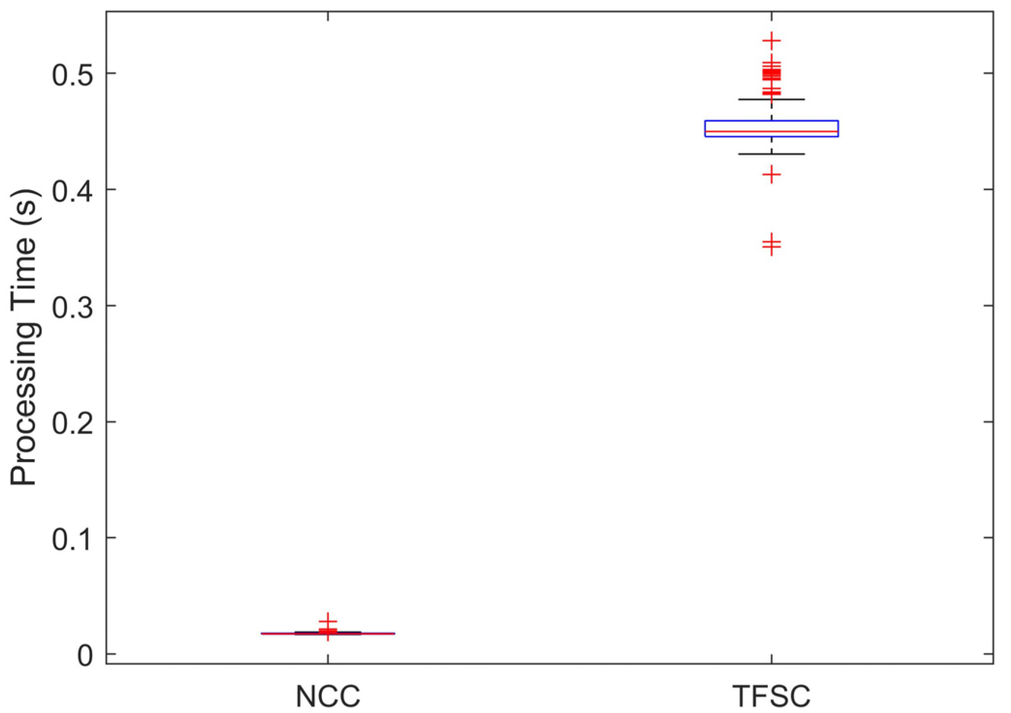
| Methods | NCC | TFSC |
|---|---|---|
| Transform domain | Time domain | Time–frequency domain |
| Execution time (seconds) | 0.02 | 0.44 |
Disclaimer/Publisher’s Note: The statements, opinions and data contained in all publications are solely those of the individual author(s) and contributor(s) and not of MDPI and/or the editor(s). MDPI and/or the editor(s) disclaim responsibility for any injury to people or property resulting from any ideas, methods, instructions or products referred to in the content. |
© 2025 by the authors. Licensee MDPI, Basel, Switzerland. This article is an open access article distributed under the terms and conditions of the Creative Commons Attribution (CC BY) license (https://creativecommons.org/licenses/by/4.0/).
Share and Cite
Yao, Y.; Xu, X.; Wang, J.; Liu, L.; Ma, Z. A Novel Time–Frequency Similarity Method for P-Wave First-Motion Polarity Detection. Sensors 2025, 25, 4157. https://doi.org/10.3390/s25134157
Yao Y, Xu X, Wang J, Liu L, Ma Z. A Novel Time–Frequency Similarity Method for P-Wave First-Motion Polarity Detection. Sensors. 2025; 25(13):4157. https://doi.org/10.3390/s25134157
Chicago/Turabian StyleYao, Yanji, Xin Xu, Jing Wang, Lintao Liu, and Zifei Ma. 2025. "A Novel Time–Frequency Similarity Method for P-Wave First-Motion Polarity Detection" Sensors 25, no. 13: 4157. https://doi.org/10.3390/s25134157
APA StyleYao, Y., Xu, X., Wang, J., Liu, L., & Ma, Z. (2025). A Novel Time–Frequency Similarity Method for P-Wave First-Motion Polarity Detection. Sensors, 25(13), 4157. https://doi.org/10.3390/s25134157