
Mitigating the Impact of Electrode Shift on Classification Performance in Electromyography Applications Using Sliding-Window Normalization


Abstract
1. Introduction
2. Methods
2.1. Data Acquisition
2.1.1. Subjects
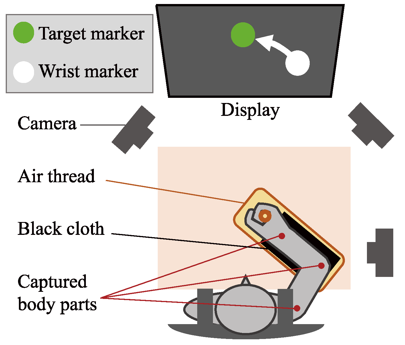
2.1.2. Experiment
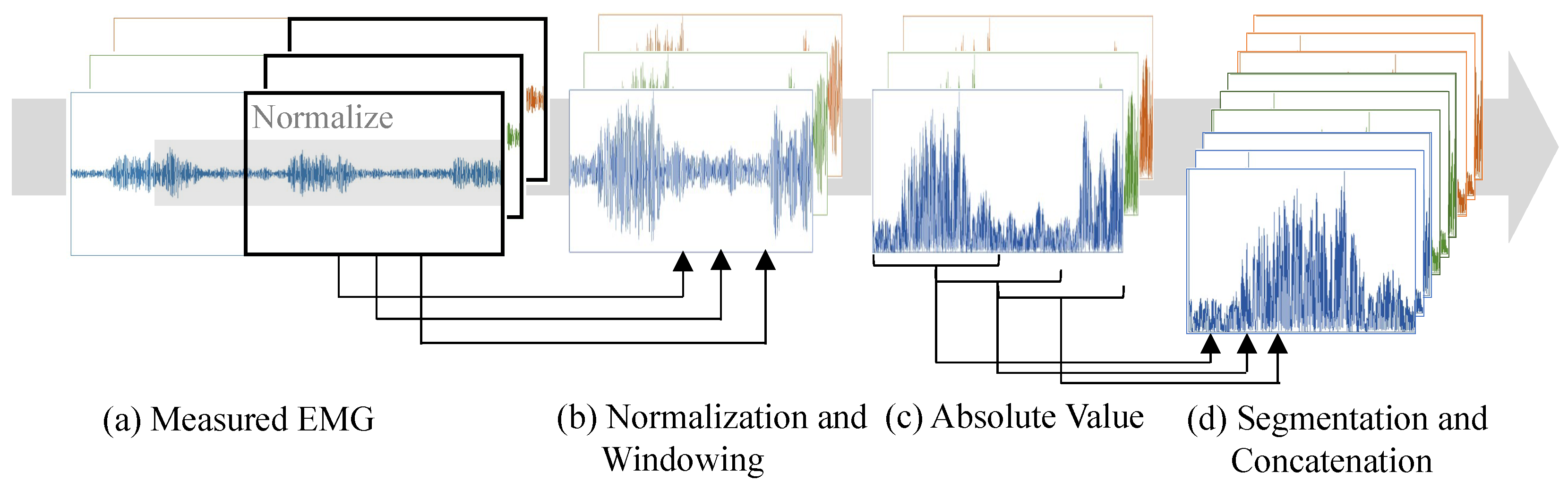
2.2. EMG Processing
2.3. Motion Labels Processing
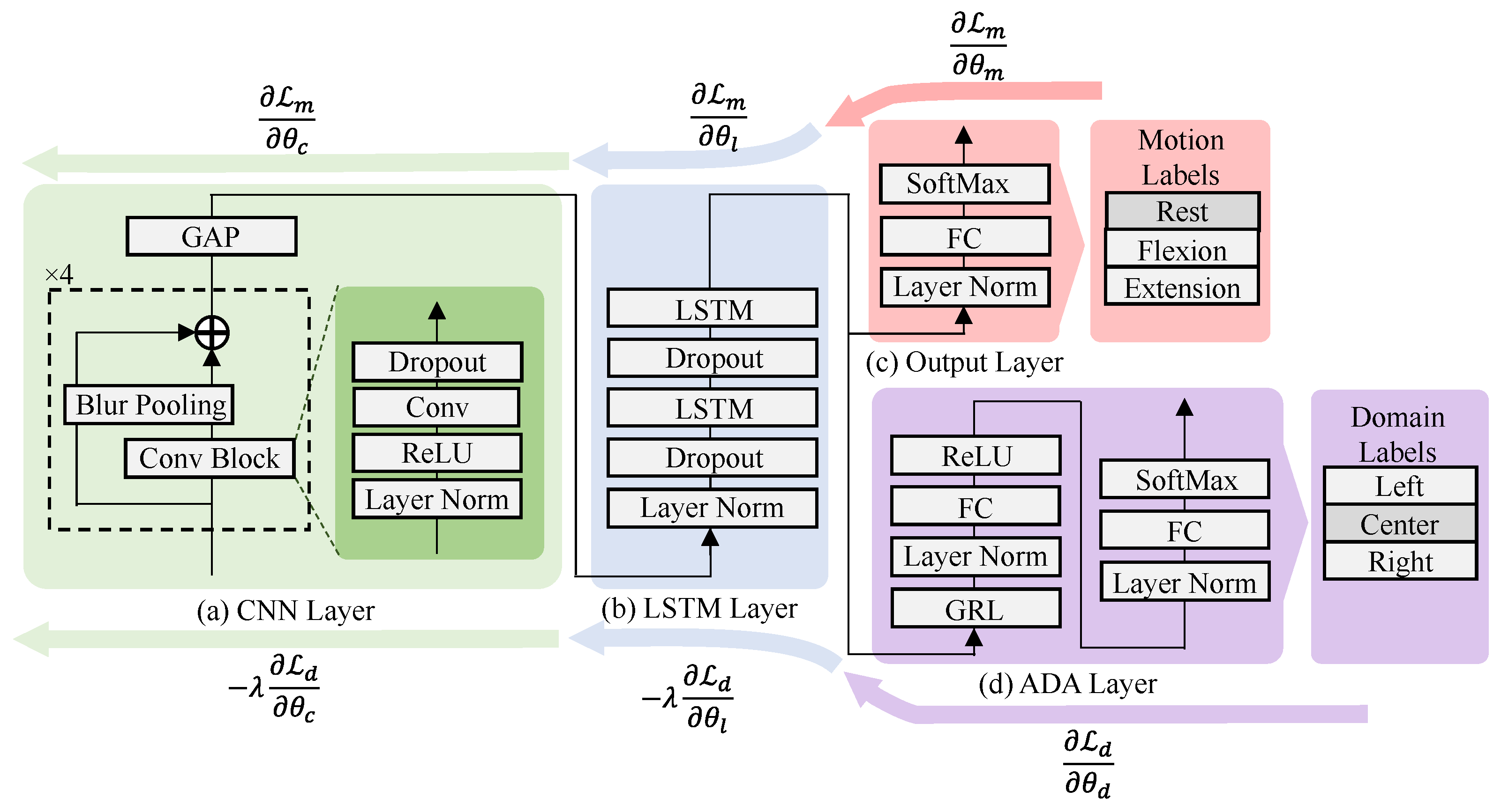
2.4. DNN Model
2.5. Comparison Methods
2.5.1. Sliding-Window Normalization (SWN)
2.5.2. Vanilla
2.5.3. Transfer Learning (TL)
2.5.4. Adversarial Domain Adaptation (ADA)
2.5.5. Mixture of Multiple Electrode Positions’ Data (MIX)
2.6. Training and Evaluation Criteria
2.6.1. Training, Tuning, and Testing Data
2.6.2. Testing Method
2.6.3. Evaluation Index
2.6.4. Statistical Analysis
3. Results
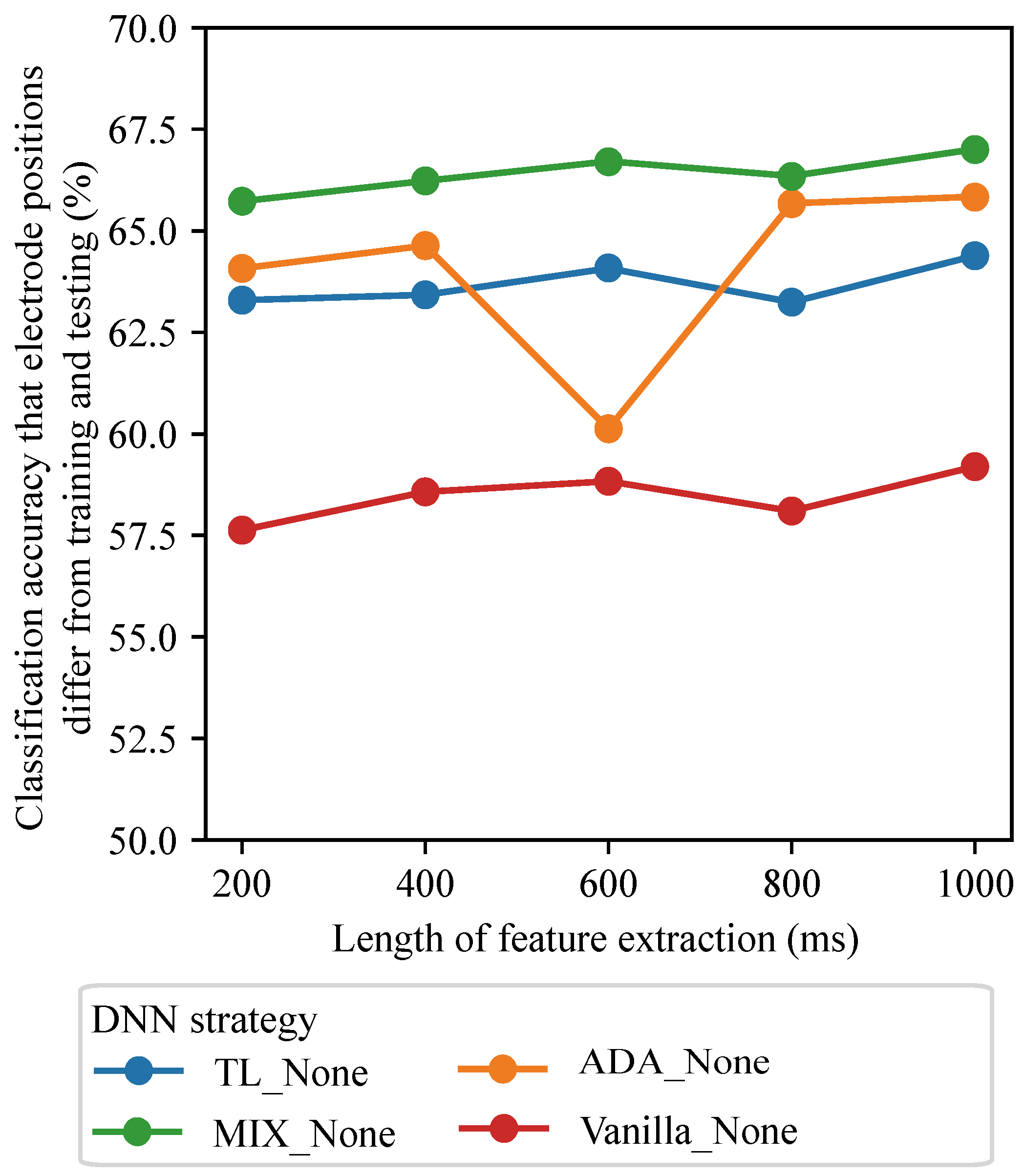
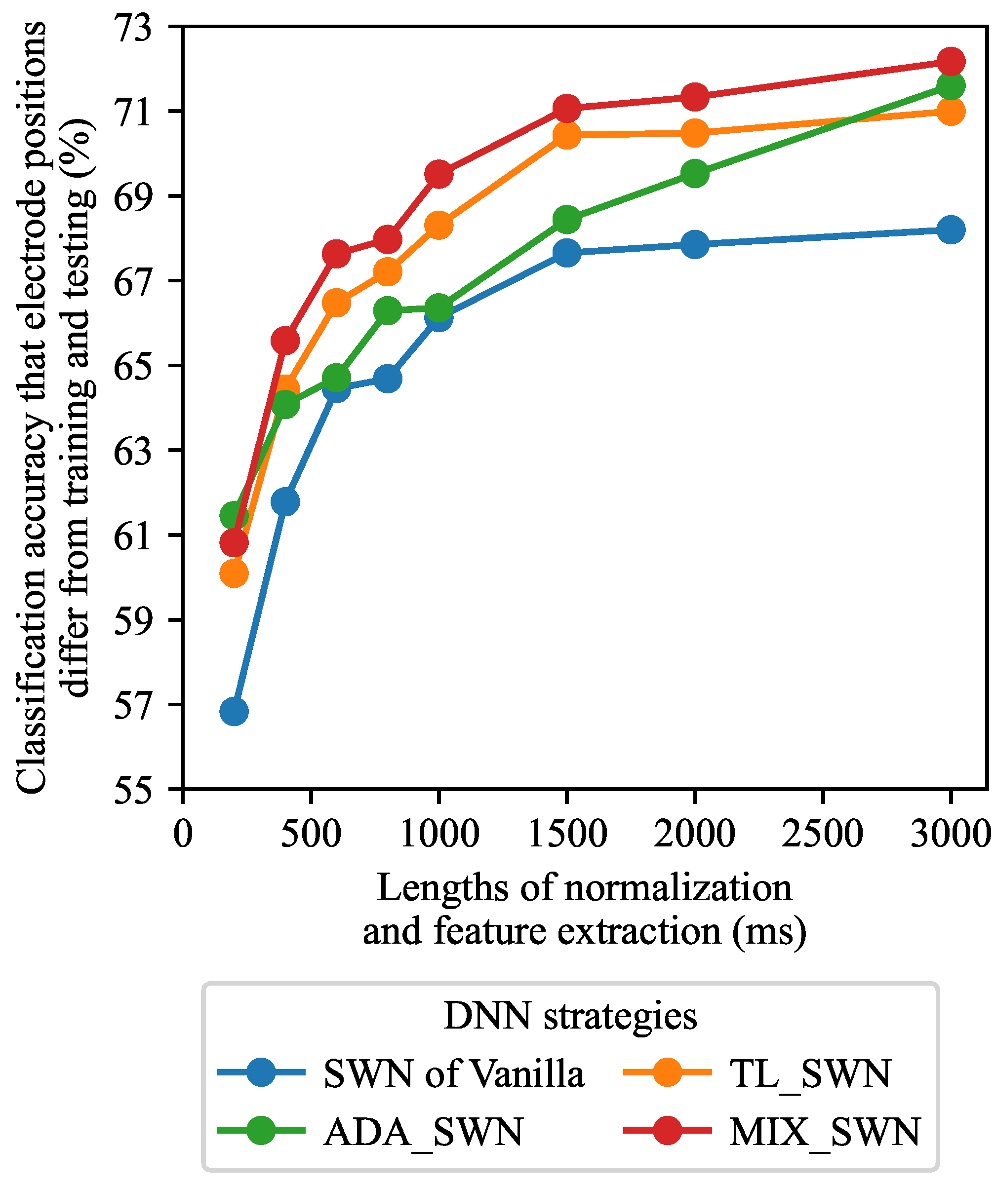
3.1. Effects of Window Lengths
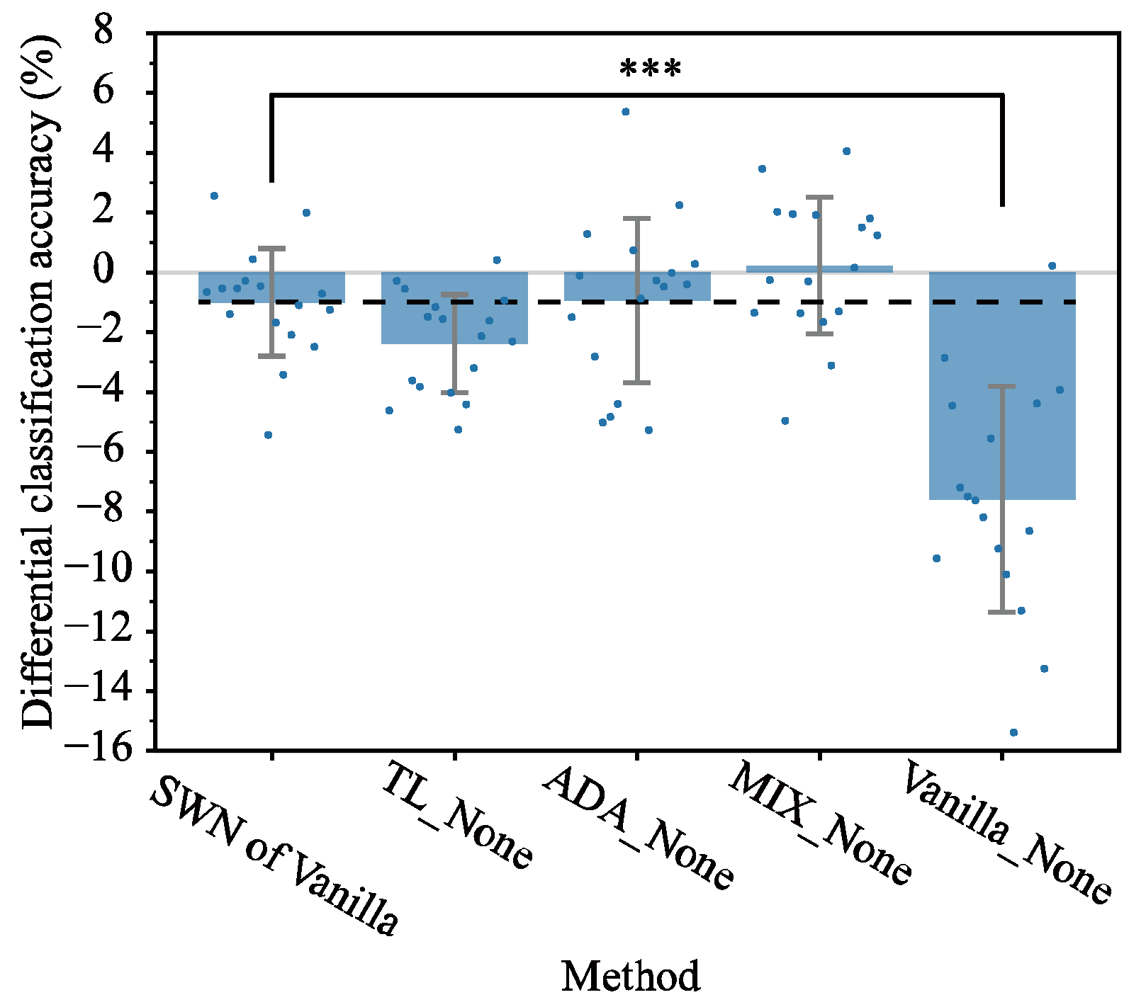
3.2. Comparison of Alternative Methods Against SWN
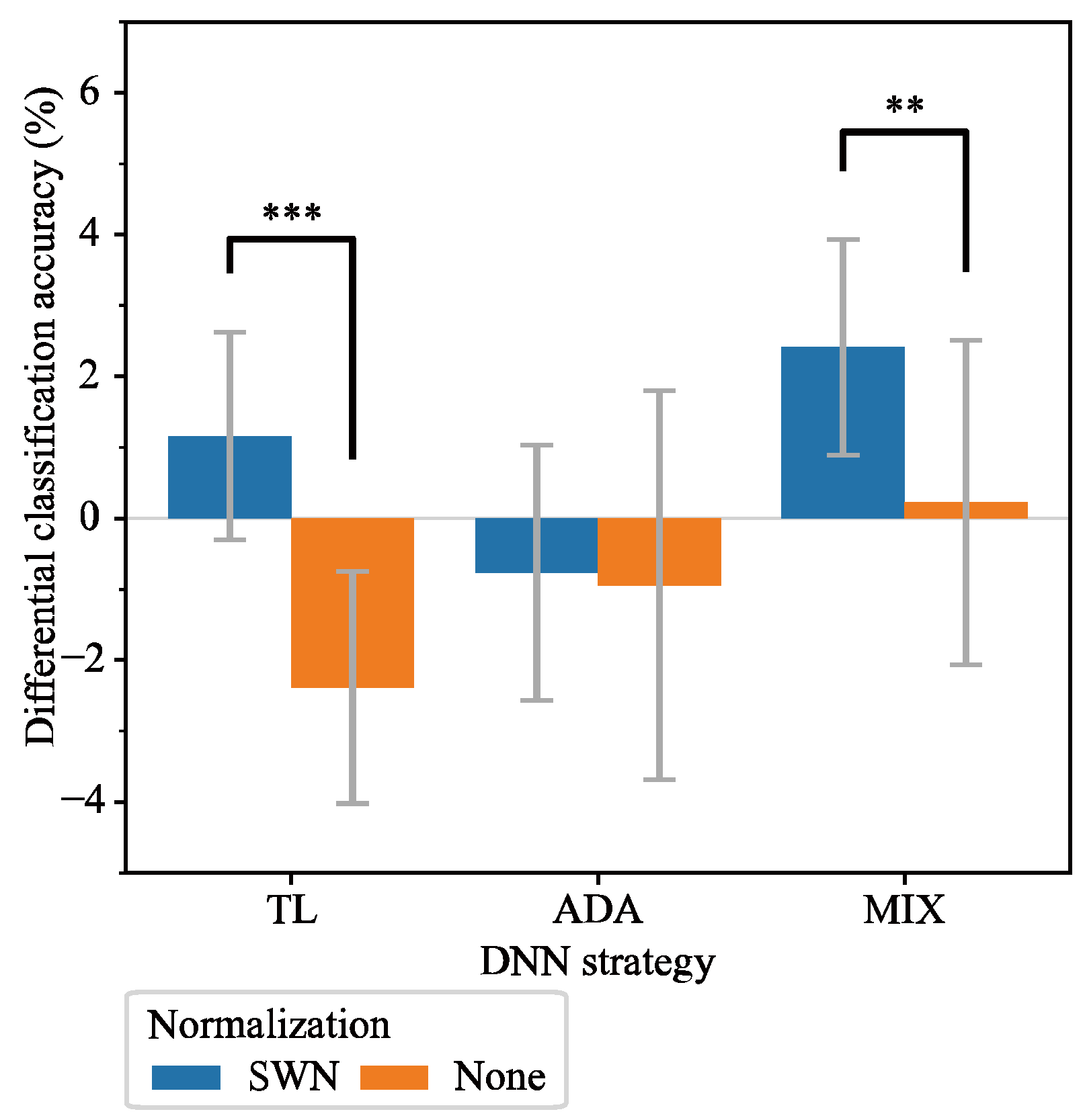
3.3. Comparison of DNN Methods with SWN Integration
4. Discussion
4.1. Performance of SWN
4.2. DNN Strategies with SWN Integration
4.3. Parameters Selection for Proposed SWN
4.4. Strengths and Limitations of SWN
5. Conclusions
Supplementary Materials
Author Contributions
Funding
Institutional Review Board Statement
Informed Consent Statement
Data Availability Statement
Conflicts of Interest
References
- Wu, C.; Song, A.; Ling, Y.; Wang, N.; Tian, L. A control strategy with tactile perception feedback for EMG prosthetic hand. J. Sens. 2015, 2015, 869175. [Google Scholar] [CrossRef]
- Atzori, M.; Cognolato, M.; Müller, H. Deep learning with convolutional neural networks applied to electromyography data: A resource for the classification of movements for prosthetic hands. Front. Neurorobotics 2016, 10, 9. [Google Scholar] [CrossRef] [PubMed]
- Dere, M.D.; Lee, B. A novel approach to surface EMG-based gesture classification using a vision transformer integrated with convolutive blind source separation. IEEE J. Biomed. Health Inform. 2023, 28, 181–192. [Google Scholar] [CrossRef] [PubMed]
- Zhang, Z.; Ming, Y.; Shen, Q.; Wang, Y.; Zhang, Y. An extended variational autoencoder for cross-subject electromyograph gesture recognition. Biomed. Signal Process. Control 2025, 99, 106828. [Google Scholar] [CrossRef]
- Yun, Y.; Na, Y.; Esmatloo, P.; Dancausse, S.; Serrato, A.; Merring, C.A.; Agarwal, P.; Deshpande, A.D. Improvement of hand functions of spinal cord injury patients with electromyography-driven hand exoskeleton: A feasibility study. Wearable Technol. 2020, 1, e8. [Google Scholar] [CrossRef]
- Phinyomark, A.; Nuidod, A.; Phukpattaranont, P.; Limsakul, C. Feature extraction and reduction of wavelet transform coefficients for EMG pattern classification. Elektron. Elektrotechnika 2012, 122, 27–32. [Google Scholar] [CrossRef]
- Omar, S.N. Application of digital signal processing and machine learning for Electromyography: A review. Asian J. Med. Technol. 2021, 1, 30–45. [Google Scholar] [CrossRef]
- Too, J.; Abdullah, A.; Saad, N.M.; Ali, N.M.; Musa, H. A detail study of wavelet families for EMG pattern recognition. Int. J. Electr. Comput. Eng. (IJECE) 2018, 8, 4221–4229. [Google Scholar] [CrossRef]
- Prahm, C.; Paassen, B.; Schulz, A.; Hammer, B.; Aszmann, O. Transfer learning for rapid re-calibration of a myoelectric prosthesis after electrode shift. In Converging Clinical and Engineering Research on Neurorehabilitation II, Proceedings of the 3rd International Conference on NeuroRehabilitation (ICNR2016), Segovia, Spain, 18–21 October 2016; Springer: Cham, Switzerland, 2016; pp. 153–157. [Google Scholar]
- Bao, T.; Zaidi, S.A.R.; Xie, S.; Yang, P.; Zhang, Z.Q. A CNN-LSTM hybrid model for wrist kinematics estimation using surface electromyography. IEEE Trans. Instrum. Meas. 2020, 70, 1–9. [Google Scholar] [CrossRef]
- Gu, X.; Guo, Y.; Deligianni, F.; Lo, B.; Yang, G.Z. Cross-subject and cross-modal transfer for generalized abnormal gait pattern recognition. IEEE Trans. Neural Netw. Learn. Syst. 2020, 32, 546–560. [Google Scholar] [CrossRef]
- Li, X.; Zhang, X.; Chen, X.; Chen, X.; Zhang, L. A unified user-generic framework for myoelectric pattern recognition: Mix-up and adversarial training for domain generalization and adaptation. IEEE Trans. Biomed. Eng. 2023, 70, 2248–2257. [Google Scholar] [CrossRef] [PubMed]
- Ameri, A.; Akhaee, M.A.; Scheme, E.; Englehart, K. A deep transfer learning approach to reducing the effect of electrode shift in EMG pattern recognition-based control. IEEE Trans. Neural Syst. Rehabil. Eng. 2019, 28, 370–379. [Google Scholar] [CrossRef] [PubMed]
- Prahm, C.; Schulz, A.; Paaßen, B.; Schoisswohl, J.; Kaniusas, E.; Dorffner, G.; Hammer, B.; Aszmann, O. Counteracting electrode shifts in upper-limb prosthesis control via transfer learning. IEEE Trans. Neural Syst. Rehabil. Eng. 2019, 27, 956–962. [Google Scholar] [CrossRef] [PubMed]
- Li, Z.; Zhao, X.; Liu, G.; Zhang, B.; Zhang, D.; Han, J. Electrode shifts estimation and adaptive correction for improving robustness of sEMG-based recognition. IEEE J. Biomed. Health Inform. 2020, 25, 1101–1110. [Google Scholar] [CrossRef]
- Côté-Allard, U.; Gagnon-Turcotte, G.; Phinyomark, A.; Glette, K.; Scheme, E.J.; Laviolette, F.; Gosselin, B. Unsupervised domain adversarial self-calibration for electromyography-based gesture recognition. IEEE Access 2020, 8, 177941–177955. [Google Scholar] [CrossRef]
- Zhai, X.; Jelfs, B.; Chan, R.H.; Tin, C. Self-recalibrating surface EMG pattern recognition for neuroprosthesis control based on convolutional neural network. Front. Neurosci. 2017, 11, 379. [Google Scholar] [CrossRef]
- Hahne, J.M.; Dähne, S.; Hwang, H.J.; Müller, K.R.; Parra, L.C. Concurrent adaptation of human and machine improves simultaneous and proportional myoelectric control. IEEE Trans. Neural Syst. Rehabil. Eng. 2015, 23, 618–627. [Google Scholar] [CrossRef]
- Hudgins, B.; Parker, P.; Scott, R.N. A new strategy for multifunction myoelectric control. IEEE Trans. Biomed. Eng. 1993, 40, 82–94. [Google Scholar] [CrossRef]
- Too, J.; Abdullah, A.R.; Saad, N.M. Classification of hand movements based on discrete wavelet transform and enhanced feature extraction. Int. J. Adv. Comput. Sci. Appl. 2019, 10. [Google Scholar] [CrossRef]
- Kim, K.T.; Guan, C.; Lee, S.W. A subject-transfer framework based on single-trial EMG analysis using convolutional neural networks. IEEE Trans. Neural Syst. Rehabil. Eng. 2019, 28, 94–103. [Google Scholar] [CrossRef]
- Wang, L.; Li, X.; Chen, Z.; Sun, Z.; Xue, J.; Sun, W.; Zhang, S. A novel hybrid unsupervised domain adaptation method for cross-subject joint angle estimation from surface electromyography. IEEE Robot. Autom. Lett. 2023, 8, 7257–7264. [Google Scholar] [CrossRef]
- Young, A.J.; Hargrove, L.J.; Kuiken, T.A. Improving myoelectric pattern recognition robustness to electrode shift by changing interelectrode distance and electrode configuration. IEEE Trans. Biomed. Eng. 2011, 59, 645–652. [Google Scholar] [CrossRef] [PubMed]
- Gao, G.; Zhang, X.; Chen, X.; Chen, Z. Mitigating the Concurrent Interference of Electrode Shift and Loosening in Myoelectric Pattern Recognition Using Siamese Autoencoder Network. IEEE Trans. Neural Syst. Rehabil. Eng. 2024, 32, 3388–3398. [Google Scholar] [CrossRef] [PubMed]
- Tanaka, T.; Nambu, I.; Maruyama, Y.; Wada, Y. Sliding-window normalization to improve the performance of machine-learning models for real-time motion prediction using electromyography. Sensors 2022, 22, 5005. [Google Scholar] [CrossRef]
- Huebner, A.; Faenger, B.; Schenk, P.; Scholle, H.C.; Anders, C. Alteration of Surface EMG amplitude levels of five major trunk muscles by defined electrode location displacement. J. Electromyogr. Kinesiol. 2015, 25, 214–223. [Google Scholar] [CrossRef]
- Mesin, L.; Merletti, R.; Rainoldi, A. Surface EMG: The issue of electrode location. J. Electromyogr. Kinesiol. 2009, 19, 719–726. [Google Scholar] [CrossRef]
- Zhang, R. Making convolutional networks shift-invariant again. In Proceedings of the International Conference on Machine Learning, PMLR, Long Beach, CA, USA, 10–15 June 2019; pp. 7324–7334. [Google Scholar]
- Lin, T.Y.; Goyal, P.; Girshick, R.; He, K.; Dollar, P. Focal Loss for Dense Object Detection. In Proceedings of the IEEE International Conference on Computer Vision (ICCV), Venice, Italy, 22–29 October 2017. [Google Scholar]
- Navallas, J.; Mariscal, C.; Malanda, A.; Rodríguez-Falces, J. Understanding EMG PDF changes with motor unit potential amplitudes, firing rates, and noise level through EMG filling curve analysis. IEEE Trans. Neural Syst. Rehabil. Eng. 2024, 32, 3240–3250. [Google Scholar] [CrossRef]
- Lin, M.W.; Ruan, S.J.; Tu, Y.W. A 3DCNN-LSTM hybrid framework for sEMG-based noises recognition in exercise. IEEE Access 2020, 8, 162982–162988. [Google Scholar] [CrossRef]
- Li, M.; Wang, J.; Yang, S.; Xie, J.; Xu, G.; Luo, S. A CNN-LSTM model for six human ankle movements classification on different loads. Front. Hum. Neurosci. 2023, 17, 1101938. [Google Scholar] [CrossRef]
- Rezaee, K.; Khavari, S.F.; Ansari, M.; Zare, F.; Roknabadi, M.H.A. Hand gestures classification of sEMG signals based on BiLSTM-metaheuristic optimization and hybrid U-Net-MobileNetV2 encoder architecture. Sci. Rep. 2024, 14, 31257. [Google Scholar] [CrossRef]
- Song, J.; Zhu, A.; Tu, Y.; Huang, H.; Arif, M.A.; Shen, Z.; Zhang, X.; Cao, G. Effects of different feature parameters of sEMG on human motion pattern recognition using multilayer perceptrons and LSTM neural networks. Appl. Sci. 2020, 10, 3358. [Google Scholar] [CrossRef]
- Chen, Y.; Yu, S.; Ma, K.; Huang, S.; Li, G.; Cai, S.; Xie, L. A continuous estimation model of upper limb joint angles by using surface electromyography and deep learning method. IEEE Access 2019, 7, 174940–174950. [Google Scholar] [CrossRef]
- Zhong, T.; Li, D.; Wang, J.; Xu, J.; An, Z.; Zhu, Y. Fusion learning for semg recognition of multiple upper-limb rehabilitation movements. Sensors 2021, 21, 5385. [Google Scholar] [CrossRef] [PubMed]
- Lin, C.; Niu, X.; Zhang, J.; Fu, X. Improving motion intention recognition for trans-radial amputees based on sEMG and transfer learning. Appl. Sci. 2023, 13, 11071. [Google Scholar] [CrossRef]
- Fan, J.; Jiang, M.; Lin, C.; Li, G.; Fiaidhi, J.; Ma, C.; Wu, W. Improving sEMG-based motion intention recognition for upper-limb amputees using transfer learning. Neural Comput. Appl. 2023, 35, 16101–16111. [Google Scholar] [CrossRef]
- Kane, G.; Lopes, G.; Sanders, J.; Mathis, A.; Mathis, M. Real-time, low-latency closed-loop feedback using markerless posture tracking. eLife 2020. Available online: https://github.com/DeepLabCut/DeepLabCut-live (accessed on 30 May 2025).
- Karashchuk, P.; Rupp, K.L.; Dickinson, E.S.; Walling-Bell, S.; Sanders, E.; Azim, E.; Brunton, B.W.; Tuthill, J.C. Anipose: A toolkit for robust markerless 3d pose estimation. Cell Rep. 2021, 36. Available online: https://anipose.readthedocs.io/en/latest/ (accessed on 30 May 2025). [CrossRef]
- Flash, T.; Hogan, N. The coordination of arm movements: An experimentally confirmed mathematical model. J. Neurosci. 1985, 5, 1688–1703. [Google Scholar] [CrossRef]


| DNN Strategy | Training Data | Tuning Data | Testing Data |
|---|---|---|---|
| Vanilla, TL | 70% of the data acquired from one electrode position | 30% of the data acquired in the Vanilla and TL common training dataset from the electrode position employed for testing (Only TL) | 30% of the data acquired from one of the different electrode positions from one used for training |
| ADA, MIX | 30% of the data acquired from each of the three electrode positions in Vanilla and TL common training dataset | - | Same common testing dataset as Vanilla and TL from one of the electrode positions |
| BASELINE | Same common training dataset as Vanilla and TL | - | Same common testing dataset as Vanilla and TL from the electrode position employed for training |
Disclaimer/Publisher’s Note: The statements, opinions and data contained in all publications are solely those of the individual author(s) and contributor(s) and not of MDPI and/or the editor(s). MDPI and/or the editor(s) disclaim responsibility for any injury to people or property resulting from any ideas, methods, instructions or products referred to in the content. |
© 2025 by the authors. Licensee MDPI, Basel, Switzerland. This article is an open access article distributed under the terms and conditions of the Creative Commons Attribution (CC BY) license (https://creativecommons.org/licenses/by/4.0/).
Share and Cite
Tanaka, T.; Nambu, I.; Wada, Y. Mitigating the Impact of Electrode Shift on Classification Performance in Electromyography Applications Using Sliding-Window Normalization. Sensors 2025, 25, 4119. https://doi.org/10.3390/s25134119
Tanaka T, Nambu I, Wada Y. Mitigating the Impact of Electrode Shift on Classification Performance in Electromyography Applications Using Sliding-Window Normalization. Sensors. 2025; 25(13):4119. https://doi.org/10.3390/s25134119
Chicago/Turabian StyleTanaka, Taichi, Isao Nambu, and Yasuhiro Wada. 2025. "Mitigating the Impact of Electrode Shift on Classification Performance in Electromyography Applications Using Sliding-Window Normalization" Sensors 25, no. 13: 4119. https://doi.org/10.3390/s25134119
APA StyleTanaka, T., Nambu, I., & Wada, Y. (2025). Mitigating the Impact of Electrode Shift on Classification Performance in Electromyography Applications Using Sliding-Window Normalization. Sensors, 25(13), 4119. https://doi.org/10.3390/s25134119