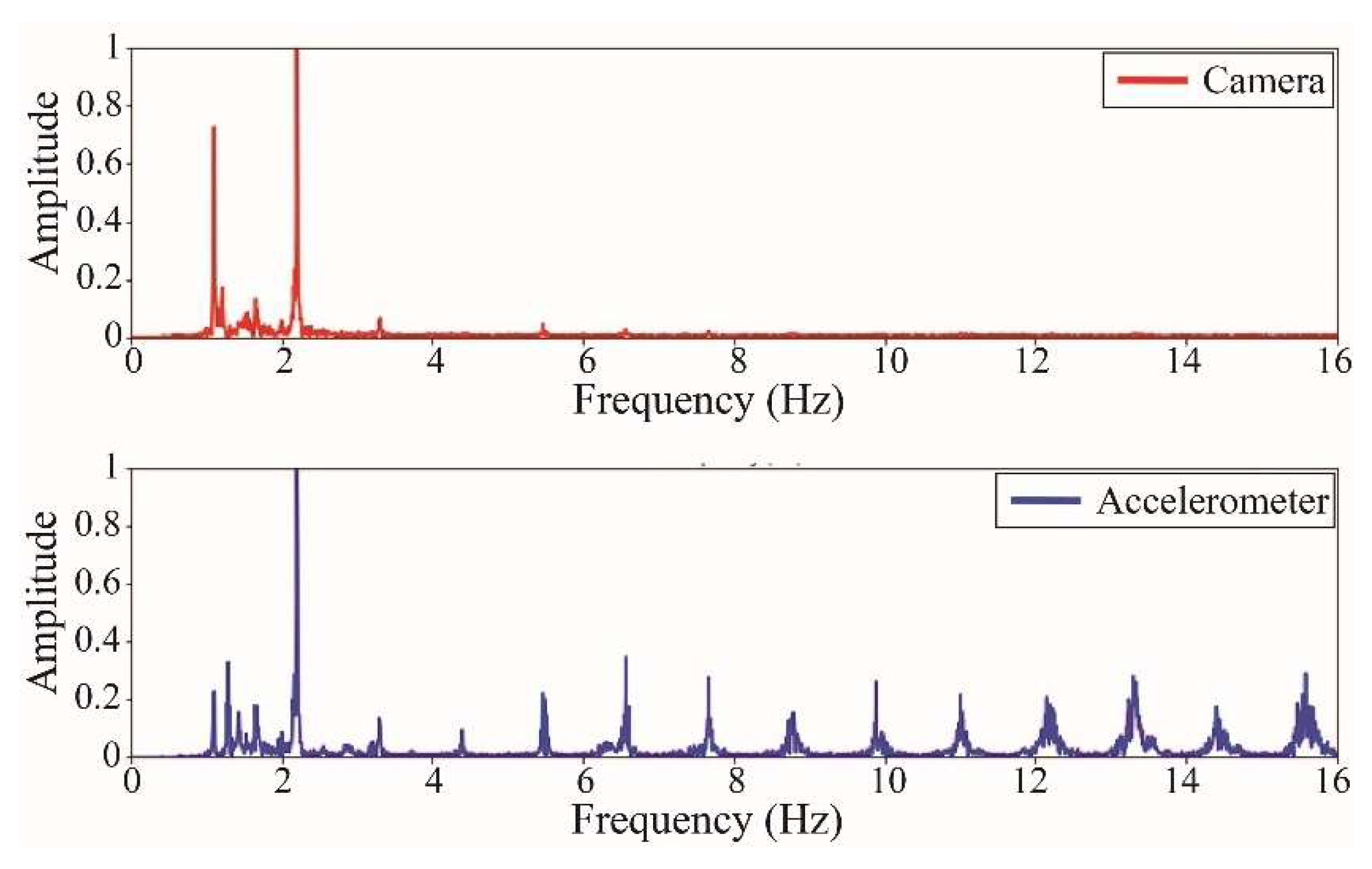
Figure 1.
Rio Papaloapan Bridge.
Figure 1.
Rio Papaloapan Bridge.
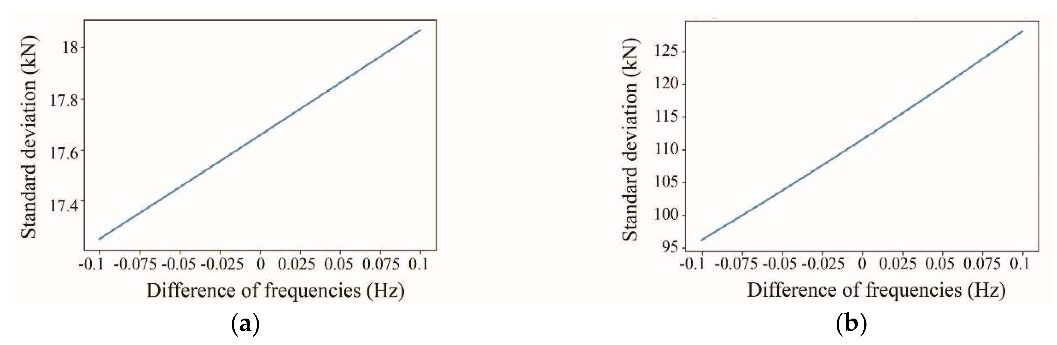
Figure 2.
Propagation error for cables: (a) on the 1st position, (b) on the 14th position.
Figure 2.
Propagation error for cables: (a) on the 1st position, (b) on the 14th position.
Figure 3.
Indirect tension force estimation for cables within the semi-harp number 5 again their maximum design limits.
Figure 3.
Indirect tension force estimation for cables within the semi-harp number 5 again their maximum design limits.
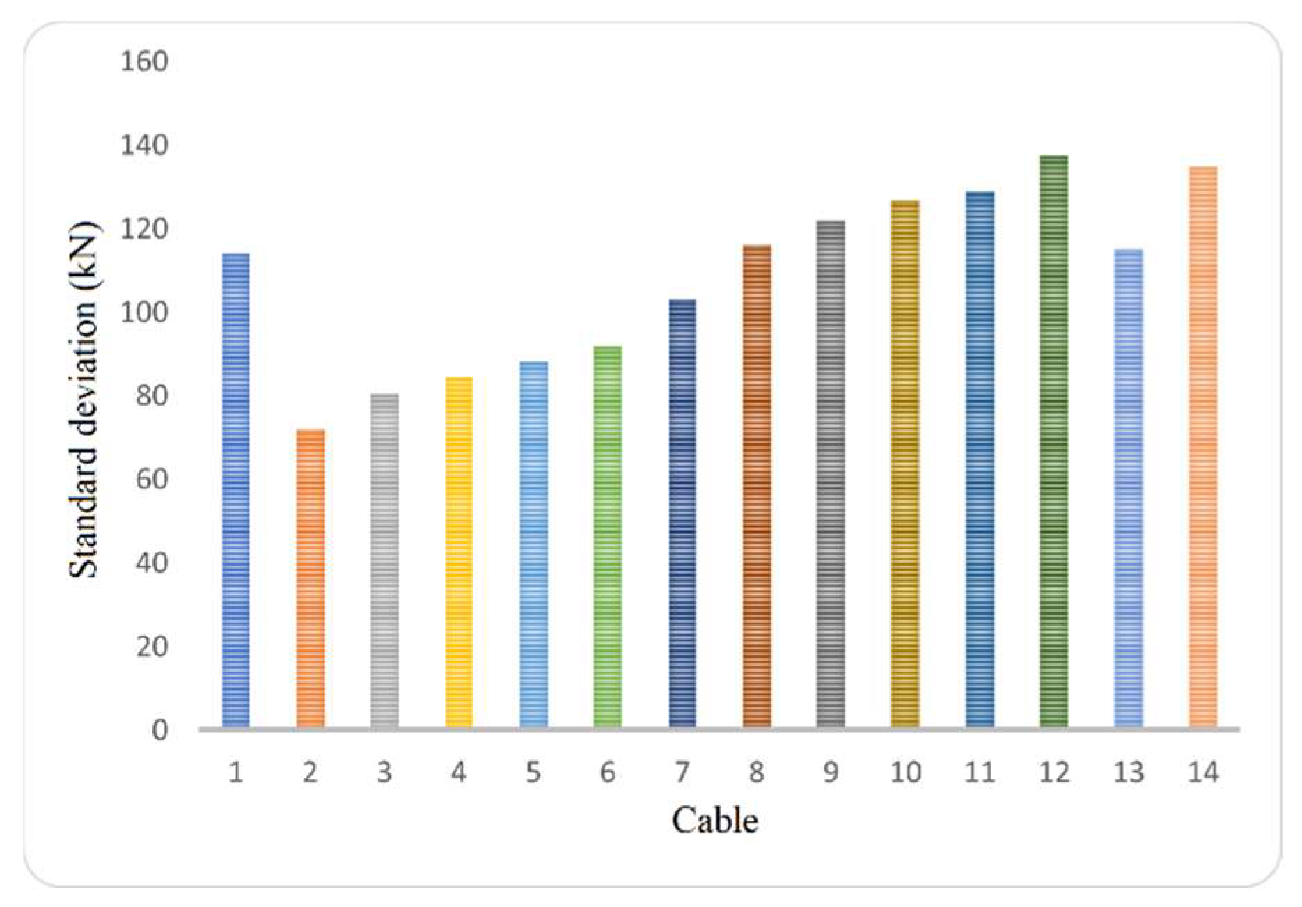
Figure 4.
Representation of the standard deviation in percentage (5%) of the total tension force.
Figure 4.
Representation of the standard deviation in percentage (5%) of the total tension force.
Figure 5.
Accelerometer on a cable during the measurement campaign.
Figure 5.
Accelerometer on a cable during the measurement campaign.
Figure 6.
Indirect tension force, direct tension force, and maximum design threshold.
Figure 6.
Indirect tension force, direct tension force, and maximum design threshold.
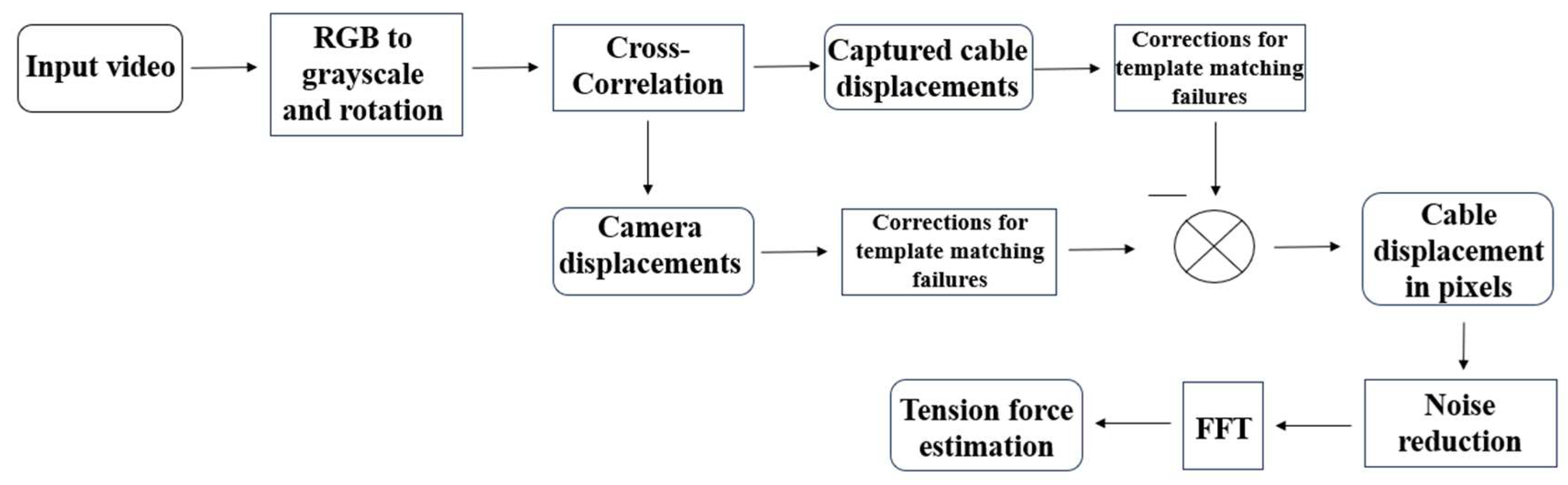
Figure 7.
Image-processing algorithm.
Figure 7.
Image-processing algorithm.
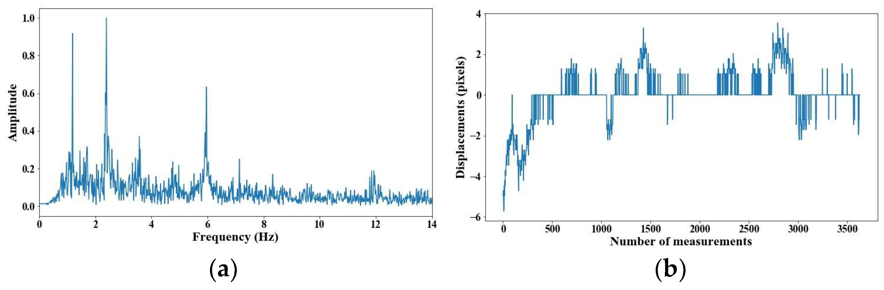
Figure 8.
Evaluation of distance, accuracy and resolution (1 m): (a) FFT; (b) displacements.
Figure 8.
Evaluation of distance, accuracy and resolution (1 m): (a) FFT; (b) displacements.
Figure 9.
Evaluation of distance, accuracy and resolution (2 m): (a) FFT; (b) displacements.
Figure 9.
Evaluation of distance, accuracy and resolution (2 m): (a) FFT; (b) displacements.
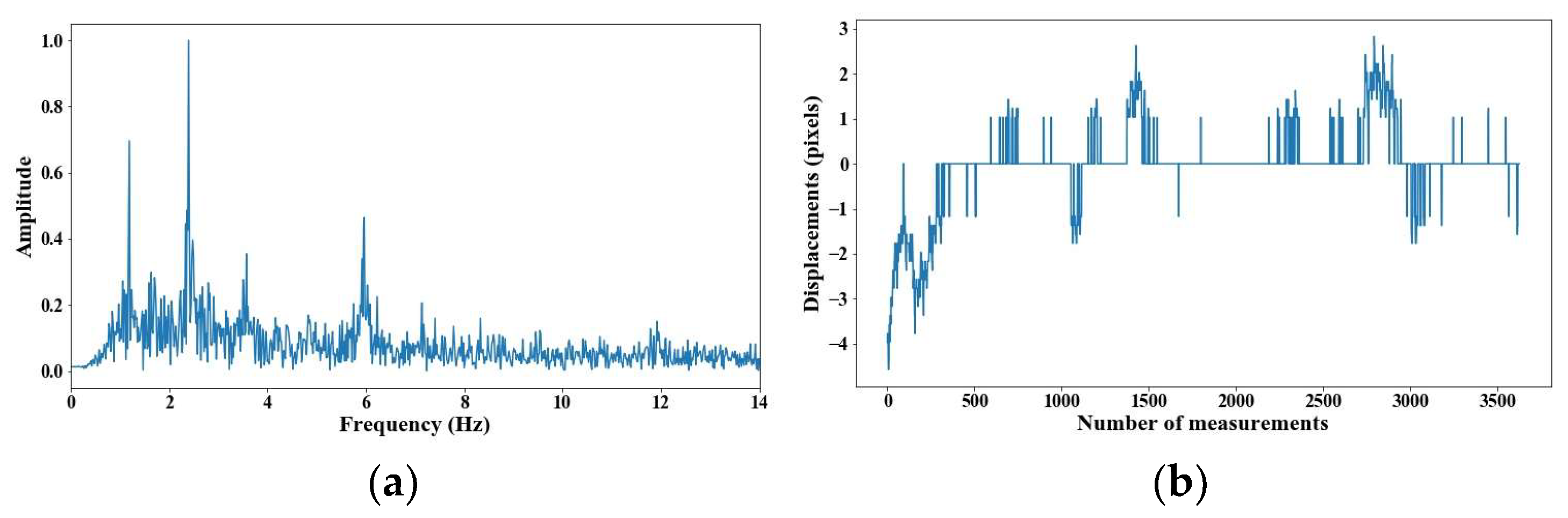
Figure 10.
Evaluation of distance, accuracy and resolution (3 m): (a) FFT; (b) displacements.
Figure 10.
Evaluation of distance, accuracy and resolution (3 m): (a) FFT; (b) displacements.
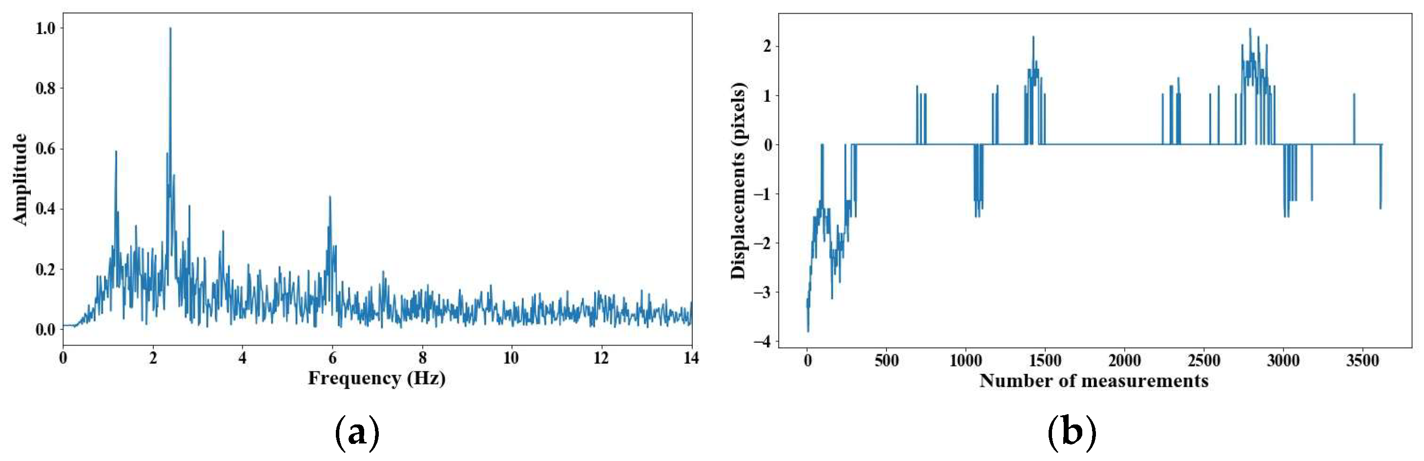
Figure 11.
Evaluation of distance, accuracy and resolution (4 m): (a) FFT; (b) displacements.
Figure 11.
Evaluation of distance, accuracy and resolution (4 m): (a) FFT; (b) displacements.
Figure 12.
Evaluation of distance, accuracy and resolution (5 m): (a) FFT; (b) displacements.
Figure 12.
Evaluation of distance, accuracy and resolution (5 m): (a) FFT; (b) displacements.
Figure 13.
Evaluation of distance, accuracy and resolution (6 m): (a) FFT; (b) displacements.
Figure 13.
Evaluation of distance, accuracy and resolution (6 m): (a) FFT; (b) displacements.
Figure 14.
Evaluation of distance, accuracy and resolution (7 m): (a) FFT; (b) displacements.
Figure 14.
Evaluation of distance, accuracy and resolution (7 m): (a) FFT; (b) displacements.
Figure 15.
Experimental validation.
Figure 15.
Experimental validation.
Figure 16.
Experimental setup at the Rio Papaloapan Bridge.
Figure 16.
Experimental setup at the Rio Papaloapan Bridge.
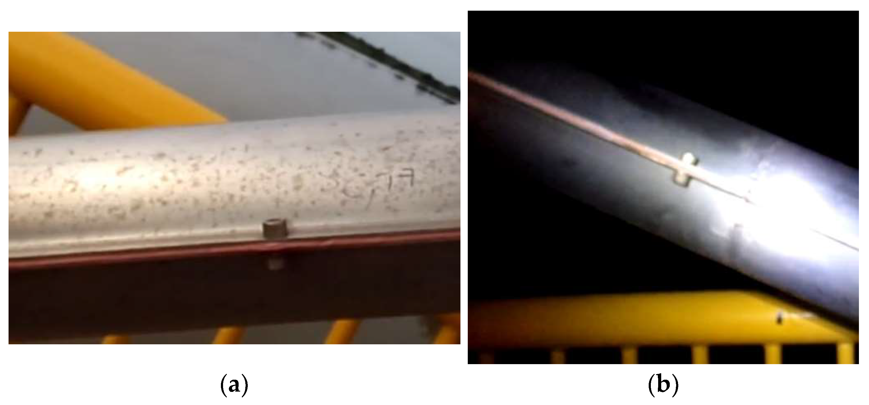
Figure 17.
Example of the different conditions during the measurements: (a) at day; (b) at dawn.
Figure 17.
Example of the different conditions during the measurements: (a) at day; (b) at dawn.
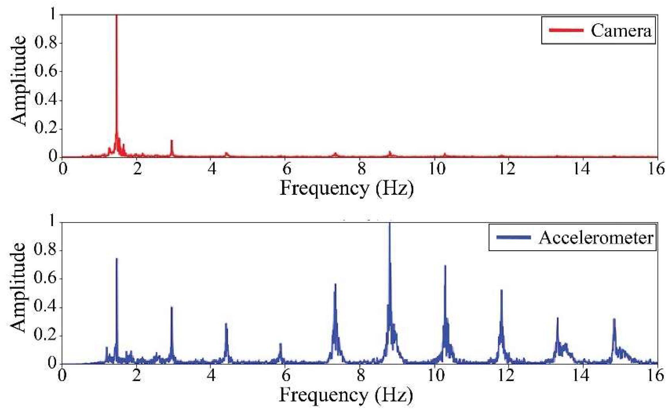
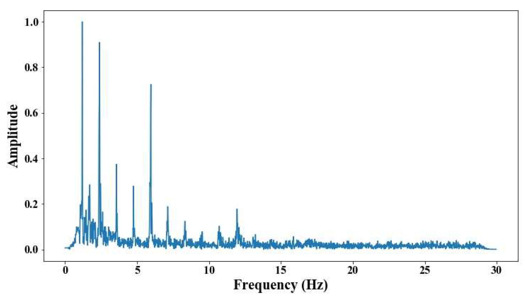
Figure 18.
Results of cable on the 14th position in frequency domain.
Figure 18.
Results of cable on the 14th position in frequency domain.
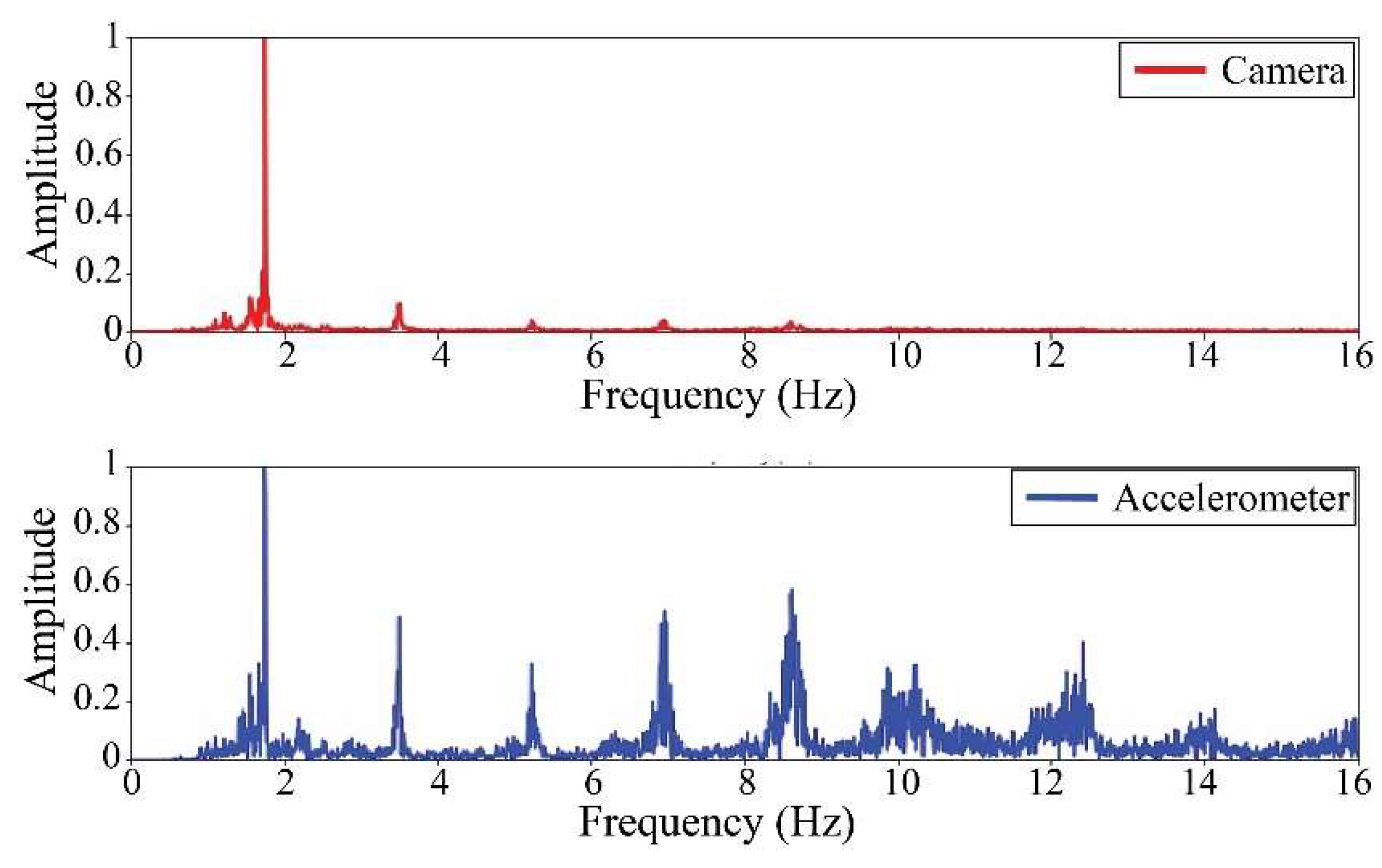
Figure 19.
Results of cable on the 12th position in frequency domain.
Figure 19.
Results of cable on the 12th position in frequency domain.
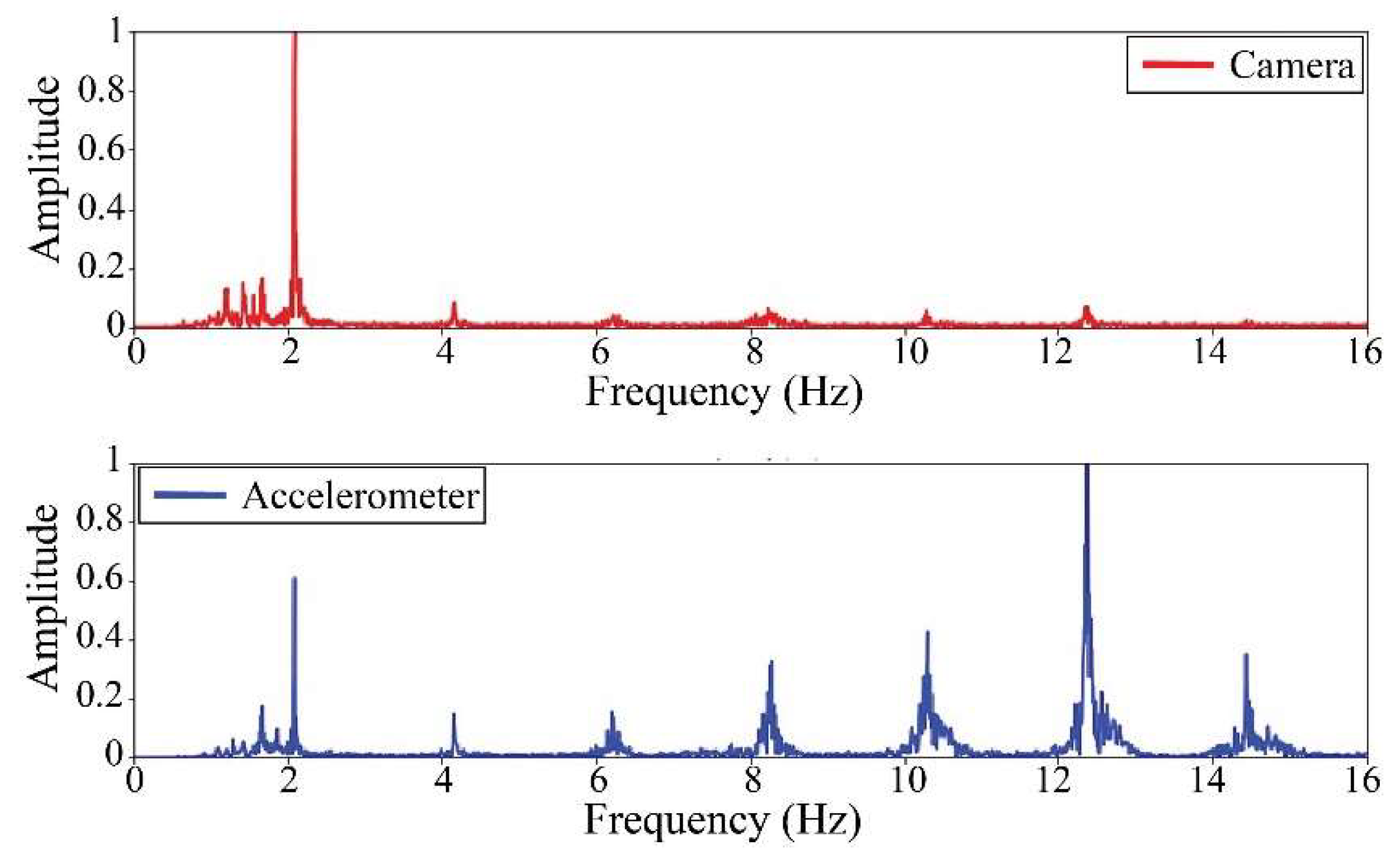
Figure 20.
Results of cable on the 10th position in frequency domain.
Figure 20.
Results of cable on the 10th position in frequency domain.
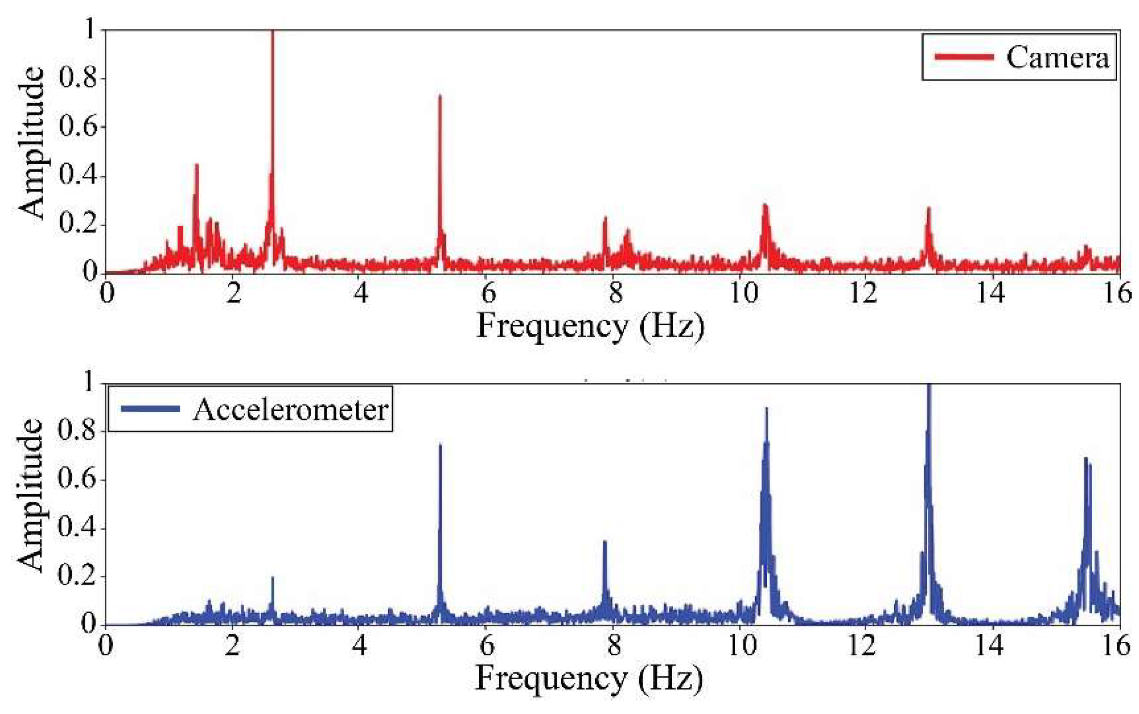
Figure 21.
Results of cable on the 8th position in frequency domain.
Figure 21.
Results of cable on the 8th position in frequency domain.
Figure 22.
Results of cable on the 6th position in frequency domain.
Figure 22.
Results of cable on the 6th position in frequency domain.
Figure 23.
Results of cable on the 5th position in frequency domain.
Figure 23.
Results of cable on the 5th position in frequency domain.
Figure 24.
Results of cable on the 4th position in frequency domain.
Figure 24.
Results of cable on the 4th position in frequency domain.
Figure 25.
Results of cable on the 2nd position in frequency domain.
Figure 25.
Results of cable on the 2nd position in frequency domain.
Figure 26.
Non-central t-Student distribution.
Figure 26.
Non-central t-Student distribution.
Figure 27.
Results of cable on the 6th position semi-harp 4 in frequency domain.
Figure 27.
Results of cable on the 6th position semi-harp 4 in frequency domain.
Figure 28.
Results of cable on the 6th position semi-harp 3 in frequency domain.
Figure 28.
Results of cable on the 6th position semi-harp 3 in frequency domain.
Figure 29.
Results of cable on the 12th position semi-harp 3 in frequency domain.
Figure 29.
Results of cable on the 12th position semi-harp 3 in frequency domain.
Figure 30.
Results of cable on the 14th position semi-harp 7 in frequency domain.
Figure 30.
Results of cable on the 14th position semi-harp 7 in frequency domain.
Figure 31.
Results of cable on the 14th position semi-harp 8 in frequency domain.
Figure 31.
Results of cable on the 14th position semi-harp 8 in frequency domain.
Table 1.
Average of frequencies in the Rio Papaloapan Bridge.
Table 1.
Average of frequencies in the Rio Papaloapan Bridge.
| Cable Position | First Mode (Hz) | Second Mode (Hz) | Third Mode (Hz) | Fourth Mode (Hz) | Fifth Mode (Hz) |
|---|
| 1 | 7.5 | 14.63 | 21.71 | 29.25 | 36.19 |
| 2 | 5.39 | 10.57 | 15.56 | 20.86 | 26.37 |
| 3 | 4.54 | 8.97 | 13.30 | 17.59 | 21.87 |
| 4 | 3.62 | 7.19 | 10.69 | 14.16 | 17.66 |
| 5 | 2.97 | 5.91 | 8.81 | 11.66 | 14.53 |
| 6 | 2.58 | 5.14 | 7.67 | 10.17 | 12.69 |
| 7 | 2.30 | 4.57 | 6.83 | 9.06 | 11.31 |
| 8 | 2.12 | 4.22 | 6.31 | 8.38 | 10.43 |
| 9 | 1.90 | 3.8 | 5.68 | 7.55 | 9.40 |
| 10 | 1.78 | 3.54 | 5.30 | 7.04 | 8.74 |
| 11 | 1.61 | 3.21 | 4.80 | 6.39 | 7.96 |
| 12 | 1.51 | 3.01 | 4.52 | 6.01 | 7.47 |
| 13 | 1.35 | 2.71 | 4.06 | 5.41 | 6.74 |
| 14 | 1.16 | 2.32 | 3.47 | 4.63 | 5.78 |
Table 2.
Analyzed cables during the validation test.
Table 2.
Analyzed cables during the validation test.
| Cable Position | Semi-Harp |
|---|
| 1 | 1 |
| 8 | 1 |
| 1 | 2 |
| 1 | 3 |
| 6 | 3 |
| 12 | 3 |
| 1 | 4 |
| 6 | 4 |
| 14 | 4 |
| 7 | 6 |
| 14 | 7 |
| 1 | 8 |
| 14 | 8 |
Table 3.
Results from the validation trial.
Table 3.
Results from the validation trial.
| Cable Position | Semi-Harp | Indirect Tension Force (kN) | Direct Tension Force (kN) | Maximum Design Threshold | Absolute
Difference (kN) | Percent Difference (%) |
|---|
| 1 | 1 | 2467.74 | 2410.8 | 2685.2 | 56.94 | 2.36 |
| 8 | 1 | 2325.24 | 2342.2 | 2920.4 | 16.96 | 0.72 |
| 1 | 2 | 2118.37 | 2146.2 | 2567.6 | 27.83 | 1.3 |
| 1 | 3 | 2014.69 | 1940.4 | 2567.6 | 74.29 | 3.8 |
| 6 | 3 | 1857.82 | 1911 | 2567.6 | 53.18 | 2.78 |
| 12 | 3 | 3001.2 | 3008.6 | 3273.2 | 7.4 | 0.25 |
| 1 | 4 | 2210.76 | 2195.2 | 2685.2 | 15.56 | 0.71 |
| 6 | 4 | 1977.01 | 1960 | 2567.6 | 17.01 | 0.87 |
| 14 | 4 | 2601.6 | 2538.2 | 3733.8 | 63.4 | 2.5 |
| 7 | 6 | 1970.3 | 1930.6 | 2802.8 | 39.7 | 2.06 |
| 14 | 7 | 2061.52 | 2028.6 | 3498.6 | 32.92 | 1.62 |
| 1 | 8 | 2286.47 | 2283.4 | 2685.2 | 3.07 | 0.13 |
| 14 | 8 | 2679.48 | 2675.4 | 3733.8 | 4.08 | 0.15 |
Table 4.
Frequency of the first vibration modes of the Rio Papaloapan Bridge.
Table 4.
Frequency of the first vibration modes of the Rio Papaloapan Bridge.
| Vibration Mode | Frequency (Hz) |
|---|
| 1 | 0.4101 |
| 2 | 0.5700 |
| 3 | 0.6471 |
| 4 | 0.7997 |
| 5 | 0.9032 |
| 6 | 0.9925 |
| 7 | 1.0978 |
| 8 | 1.1985 |
| 9 | 1.4149 |
| 10 | 1.6785 |
| 11 | 1.7655 |
| 12 | 1.9794 |
| 13 | 2.5574 |
| 14 | 2.7993 |
Table 5.
Frequency of the first vibration modes according to the camera-to-cable distance.
Table 5.
Frequency of the first vibration modes according to the camera-to-cable distance.
| Vibration Mode | Frequencies Found in 1 m of Distance (Hz) | Frequencies Found in 2 m of Distance (Hz) | Frequencies Found in 3 m of Distance (Hz) | Frequencies Found in 4 m of Distance (Hz) | Frequencies Found in 5 m of Distance (Hz) |
|---|
| 1 | 1.1923 | 1.1923 | 1.1923 | 1.192 | 1.192 |
| 2 | 2.4013 | 2.4013 | 2.4013 | 2.4006 | 2.4006 |
| 3 | 3.5774 | 3.5771 | 3.5771 | 3.5761 | 3.5761 |
| 4 | 4.7695 | 4.7695 | 4.7695 | -- | -- |
| 5 | 5.9784 | 5.9784 | 5.9784 | 5.9768 | 5.9765 |
| 6 | 7.1543 | 7.1542 | 7.1542 | 7.1523 | -- |
Table 6.
Tension force estimation considering a distance between the camera and cable of 1, 2, 3, 4, 5, 6, and 7 m.
Table 6.
Tension force estimation considering a distance between the camera and cable of 1, 2, 3, 4, 5, 6, and 7 m.
| Distance (m) | Tension Force (kN) |
|---|
| 1 | 2781.43 |
| 2 | 2781.33 |
| 3 | 2781.33 |
| 4 | 2781.61 |
| 5 | 2784.22 |
| 6 | 2783.62 |
| 7 | 2809.40 |
Table 7.
Critical technical specifications used during the laboratory validation phase.
Table 7.
Critical technical specifications used during the laboratory validation phase.
| Technical Specifications | Technical Specifications |
|---|
| Vibration frequency | 11.31, 12.69, 14.53, 17.66, 21.87, 26.37 Hz |
| Acceleration | 10 m/s2 |
| Distance camera to vibrating table | 70 cm |
| Sampling frequency | 60 fps |
| Resolution | 3840 × 2160 pixels |
| Duration session | 2 min |
Table 8.
Experimental results from the laboratory trial.
Table 8.
Experimental results from the laboratory trial.
| Test Number | Frequency of the Vibratory Table (Hz) | Acceleration of the Vibratory Test (m/s2) | Frequency Probated by the Camera (Hz) | Absolute
Difference (Hz) | Percent Difference (%) |
|---|
| 1 | 26.37 | 10 | 26.3729 | 0.0029 | 0.01 |
| 2 | 26.37 | 10 | 26.3726 | 0.0026 | 0.009 |
| 3 | 26.37 | 10 | 26.3689 | 0.0011 | 0.004 |
| 4 | 21.87 | 10 | 21.8731 | 0.0031 | 0.014 |
| 5 | 21.87 | 10 | 21.8716 | 0.0016 | 0.007 |
| 6 | 21.87 | 10 | 21.8701 | 1 × 10⁻⁴ | 0.0004 |
| 7 | 17.66 | 10 | 17.6594 | 0.0006 | 0.003 |
| 8 | 17.66 | 10 | 17.6605 | 0.0005 | 0.002 |
| 9 | 17.66 | 10 | 17.6625 | 0.0025 | 0.014 |
| 10 | 14.53 | 10 | 14.5286 | 0.0014 | 0.009 |
| 11 | 14.53 | 10 | 14.5268 | 0.0032 | 0.022 |
| 12 | 14.53 | 10 | 14.5306 | 0.0006 | 0.0041 |
| 13 | 12.69 | 10 | 12.692 | 0.002 | 0.0157 |
| 14 | 12.69 | 10 | 12.6854 | 0.0046 | 0.0362 |
| 15 | 12.69 | 10 | 12.6927 | 0.0027 | 0.021 |
| 16 | 11.31 | 10 | 11.31 | 0 | 0 |
| 17 | 11.31 | 10 | 11.308 | 0.002 | 0.0176 |
| 18 | 11.31 | 10 | 11.3075 | 0.0025 | 0.0221 |
Table 9.
Standard deviation of the laboratory trial.
Table 9.
Standard deviation of the laboratory trial.
| Frequency of the Vibratory Table (Hz) | Standard Deviation (Hz) |
|---|
| 26.37 | 0.0022 |
| 21.87 | 0.0015 |
| 17.66 | 0.0016 |
| 14.53 | 0.0019 |
| 12.69 | 0.0040 |
| 11.31 | 0.0013 |
Table 10.
Mechanical characteristics of the evaluated cables.
Table 10.
Mechanical characteristics of the evaluated cables.
| Cable Position | Semi-Harp Number | Number of Wire Strand | Dimensions (m) | Mass (kg/m) | Cable Position |
|---|
| 14 | 2 | 30 | 108.09 | 36 | 14 |
| 12 | 2 | 28 | 93.74 | 34 | 12 |
| 10 | 2 | 27 | 79.46 | 33 | 10 |
| 8 | 2 | 25 | 65.26 | 30 | 8 |
| 6 | 2 | 22 | 51.23 | 27 | 6 |
| 5 | 2 | 21 | 44.33 | 25 | 5 |
| 4 | 2 | 19 | 37.55 | 23 | 4 |
| 2 | 2 | 14 | 24.64 | 17 | 2 |
| 14 | 8 | 32 | 108.09 | 39 | 14 |
| 14 | 7 | 30 | 108.09 | 37 | 14 |
| 12 | 3 | 28 | 93.74 | 34 | 12 |
| 6 | 4 | 22 | 51.23 | 27 | 6 |
| 6 | 3 | 22 | 51.23 | 27 | 6 |
| 1 | 8 | 23 | 18.38 | 28 | 1 |
| 1 | 2 | 22 | 18.38 | 27 | 1 |
| 12 | 2 | 28 | 93.74 | 34 | 12 |
Table 11.
Results from the first Rio Papaloapan Bridge trial.
Table 11.
Results from the first Rio Papaloapan Bridge trial.
| Cable on the 14th position Semi-Harp 2 |
| Instruments | 1 (Hz) | 2 (Hz) | 3 (Hz) | 4 (Hz) | 5 (Hz) | Mean (Hz) | Results (kN) |
| Camera | 1.1066 | 2.2059 | 3.3126 | 4.4629 | 5.4749 | 1.1041 | 2165.1 |
| Accelerometer | 1.10635 | 2.205522 | 3.31904 | 4.40297 | 5.47194 | 1.10037 | 2154.2 |
| Cable on the 12th position Semi-Harp 2 |
| Instruments | 1 (Hz) | 2 (Hz) | 3 (Hz) | 4 (Hz) | 5 (Hz) | Mean (Hz) | Results (kN) |
| Camera | 1.4869 | 2.959 | 4.4239 | --- | 7.3535 | 1.4748 | 2806.36 |
| Accelerometer | 1.48294 | 2.9658 | 4.4339 | 5.88727 | 7.35538 | 1.4750 | 2804.02 |
| Cable on the 10th position Semi-Harp 2 |
| Instruments | 1 (Hz) | 2 (Hz) | 3 (Hz) | 4 (Hz) | 5 (Hz) | Mean (Hz) | Results (kN) |
| Camera | 1.7527 | 3.4981 | 5.2214 | 6.9594 | 8.6238 | 1.7370 | 2649.69 |
| Accelerometer | 1.75105 | 3.49455 | 5.2305 | 6.90607 | 8.60428 | 1.73243 | 2639.02 |
| Cable on the 8th position Semi-Harp 2 |
| Instruments | 1 (Hz) | 2 (Hz) | 3 (Hz) | 4 (Hz) | 5 (Hz) | Mean (Hz) | Results (kN) |
| Camera | 2.0940 | 4.1659 | 6.2305 | 8.2364 | 10.2936 | 2.0680 | 2328.16 |
| Accelerometer | 2.0915 | 4.1679 | 6.2215 | 8.2676 | 10.2758 | 2.06829 | 2328.03 |
| Cable on the 6th position Semi-Harp 2 |
| Instruments | 1 (Hz) | 2 (Hz) | 3 (Hz) | 4 (Hz) | 5 (Hz) | Mean (Hz) | Results (kN) |
| Camera | 2.6544 | 5.2945 | 7.9130 | 10.4096 | 13.0067 | 2.6185 | 2029.44 |
| Accelerometer | 2.65236 | 5.2975 | 7.89204 | 10.4505 | 12.9727 | 2.61767 | 2028.16 |
| Cable on the 5th position Semi-Harp 2 |
| Instruments | 1 (Hz) | 2 (Hz) | 3 (Hz) | 4 (Hz) | 5 (Hz) | Mean (Hz) | Results (kN) |
| Camera | 3.1258 | 6.2077 | 9.2384 | 12.2471 | 15.2778 | 3.07312 | 2010 |
| Accelerometer | 3.13029 | 6.20854 | 9.24217 | 12.2312 | 15.2797 | 3.07279 | 2010.69 |
| Cable on the 4th position Semi-Harp 2 |
| Instruments | 1 (Hz) | 2 (Hz) | 3 (Hz) | 4 (Hz) | 5 (Hz) | Mean (Hz) | Results (kN) |
| Camera | 3.8909 | 7.6866 | 11.3798 | 15.0656 | --- | 3.8022 | 2005.04 |
| Accelerometer | 3.88985 | 7.69211 | 11.3776 | 15.0631 | 18.5735 | 3.77308 | 1982.56 |
| Cable on the 2nd position Semi-Harp 2 |
| Instruments | 1 (Hz) | 2 (Hz) | 3 (Hz) | 4 (Hz) | 5 (Hz) | Mean (Hz) | Results (kN) |
| Camera | 5.4917 | 10.7268 | 15.7127 | --- | --- | 5.3218 | 1281.92 |
| Accelerometer | 5.49044 | 10.7236 | 15.7143 | 20.7931 | 25.8352 | 5.23711 | 1247.39 |
Table 12.
Summary of the results from the first Rio Papaloapan Bridge trial.
Table 12.
Summary of the results from the first Rio Papaloapan Bridge trial.
| Cable Position | Number of Vibration Modes | Frequencies Standard Deviation | Mean Difference (Hz) | Tension Difference (kN) | Percent Difference (%) |
|---|
| 14 | 5 | 0.0301 | 0.0037 | 10.9 | 0.51 |
| 12 | 4 | 0.0074 | 0.0002 | 2.34 | 0.08 |
| 10 | 5 | 0.0288 | 0.00457 | 10.67 | 0.40 |
| 8 | 5 | 0.0185 | 0.00029 | 0.13 | 0.01 |
| 6 | 5 | 0.0286 | 0.00083 | 1.28 | 0.06 |
| 5 | 5 | 0.0085 | 0.00033 | 0.69 | 0.03 |
| 4 | 4 | 0.0037 | 0.0291 | 22.48 | 1.13 |
| 2 | 3 | 0.0026 | 0.0846 | 34.53 | 2.77 |
Table 13.
Results of the measurement developed at dawn.
Table 13.
Results of the measurement developed at dawn.
| Cable on the 14th position Semi-Harp 8 |
| Instruments | 1 (Hz) | 2 (Hz) | 3 (Hz) | 4 (Hz) | 5 (Hz) | Mean (Hz) | Results (kN) |
| Camera | 1.1894 | 2.3953 | 3.5682 | 4.7576 | 5.9635 | 1.4199 | 2649.97 |
| Accelerometer | 1.1969 | 2.4021 | 3.6156 | 4.7543 | 5.9927 | 1.1974 | 2679.48 |
| Cable on the 14th position Semi-Harp 7 |
| Instruments | 1 (Hz) | 2 (Hz) | 3 (Hz) | 4 (Hz) | 5 (Hz) | Mean (Hz) | Results (kN) |
| Camera | 1.0658 | 2.1017 | 3.1676 | 4.2185 | 5.2693 | 1.0548 | 1999.77 |
| Accelerometer | 1.0722 | 2.1527 | 3.2 | 4.2971 | 5.3278 | 1.0699 | 2061.52 |
| Cable on the 12th position Semi-Harp 3 |
| Instruments | 1 (Hz) | 2 (Hz) | 3 (Hz) | 4 (Hz) | 5 (Hz) | Mean (Hz) | Results (kN) |
| Camera | 1.5653 | 3.141 | 4.6959 | 6.2612 | 7.7725 | 1.5624 | 3083.2 |
| Accelerometer | 1.5377 | 3.1086 | 4.6296 | 6.1423 | 7.7216 | 1.5426 | 3001.2 |
| Cable on the 6th position Semi-Harp 4 |
| Instruments | 1 (Hz) | 2 (Hz) | 3 (Hz) | 4 (Hz) | 5 (Hz) | Mean (Hz) | Results (kN) |
| Camera | 2.6204 | 5.135 | 7.676 | 10.1377 | 12.6523 | 2.5481 | 1959.53 |
| Accelerometer | 2.6099 | 5.1616 | 7.7216 | 10.1735 | 12.7086 | 2.5583 | 1977.01 |
| Cable on the 6th position Semi-Harp 3 |
| Instruments | 1 (Hz) | 2 (Hz) | 3 (Hz) | 4 (Hz) | 5 (Hz) | Mean (Hz) | Results (kN) |
| Camera | 2.5079 | -- | 7.4266 | 9.8374 | -- | 2.4714 | 1852.06 |
| Accelerometer | 2.5101 | 4.9704 | 7.4389 | 9.8577 | 12.3512 | 2.4752 | 1857.82 |
Table 14.
Summary of the results found during the measurements at dawn.
Table 14.
Summary of the results found during the measurements at dawn.
| Cable Position | Number of Semi-Harps | Number of Vibration Modes | Tension Difference (kN) | Percent Difference (%) |
|---|
| 14 | 8 | 5 | 29.51 | 1.1 |
| 14 | 7 | 5 | 61.7 | 2.9 |
| 12 | 3 | 5 | 82 | 2.7 |
| 6 | 4 | 5 | 17.48 | 0.8 |
| 6 | 3 | 3 | 5.76 | 0.3 |


 ,
, 


