
Field Testing of a Controlled-Source Wide Frequency Range Magnetotelluric Detector Using SQUID and Inductive Magnetic Sensors

 ,
,
Abstract
1. Introduction
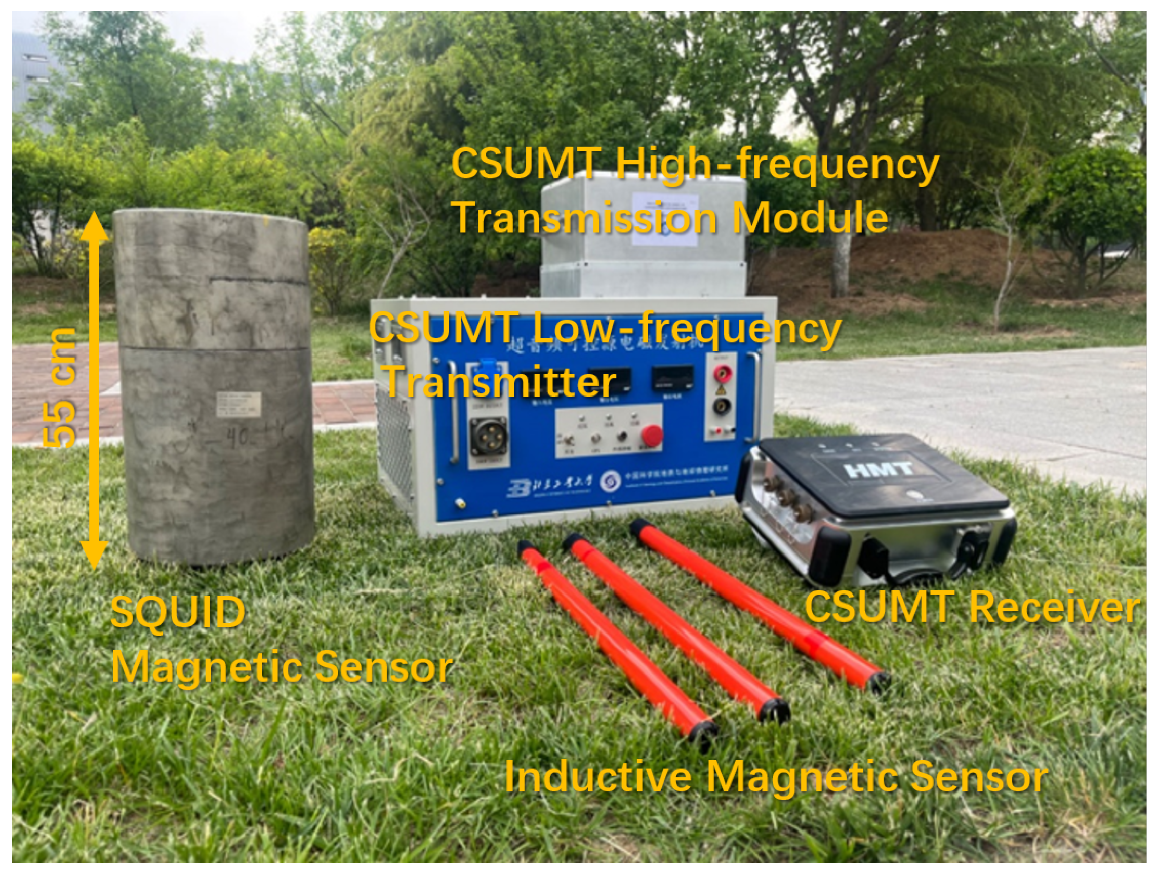
2. CSUMT Detector
3. Comparison Experiment Conducted in Shaanxi Province
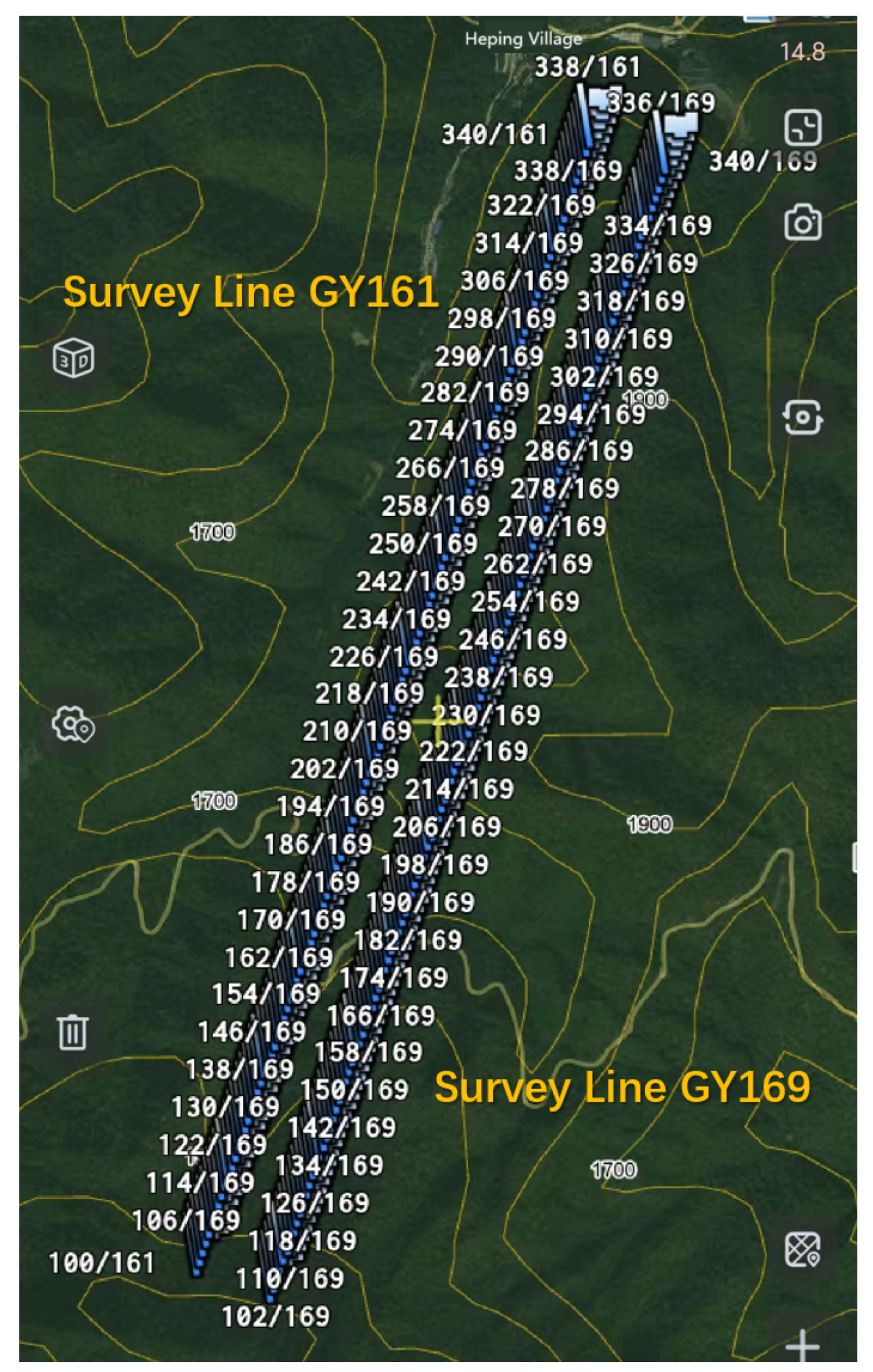
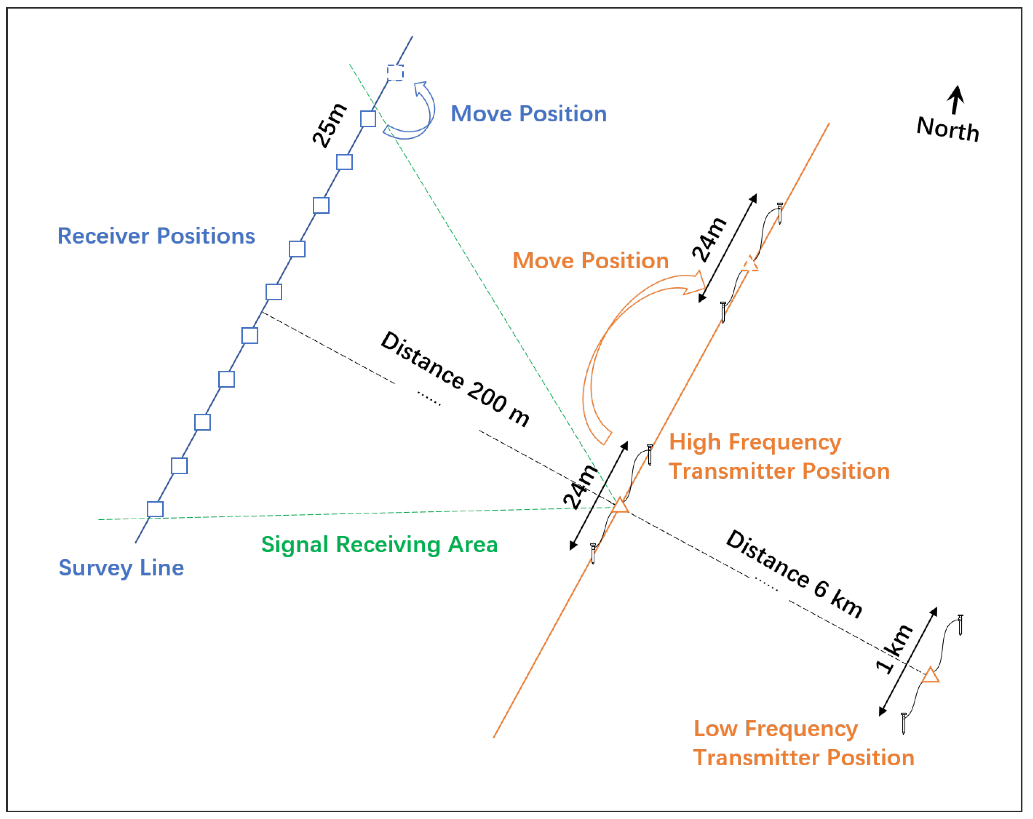
3.1. Test Design and Field Work
3.2. Comparison Experiment Results
4. Comparison Experiment Between the Inductive Magnetic Sensor and the SQUID Magnetic Sensor
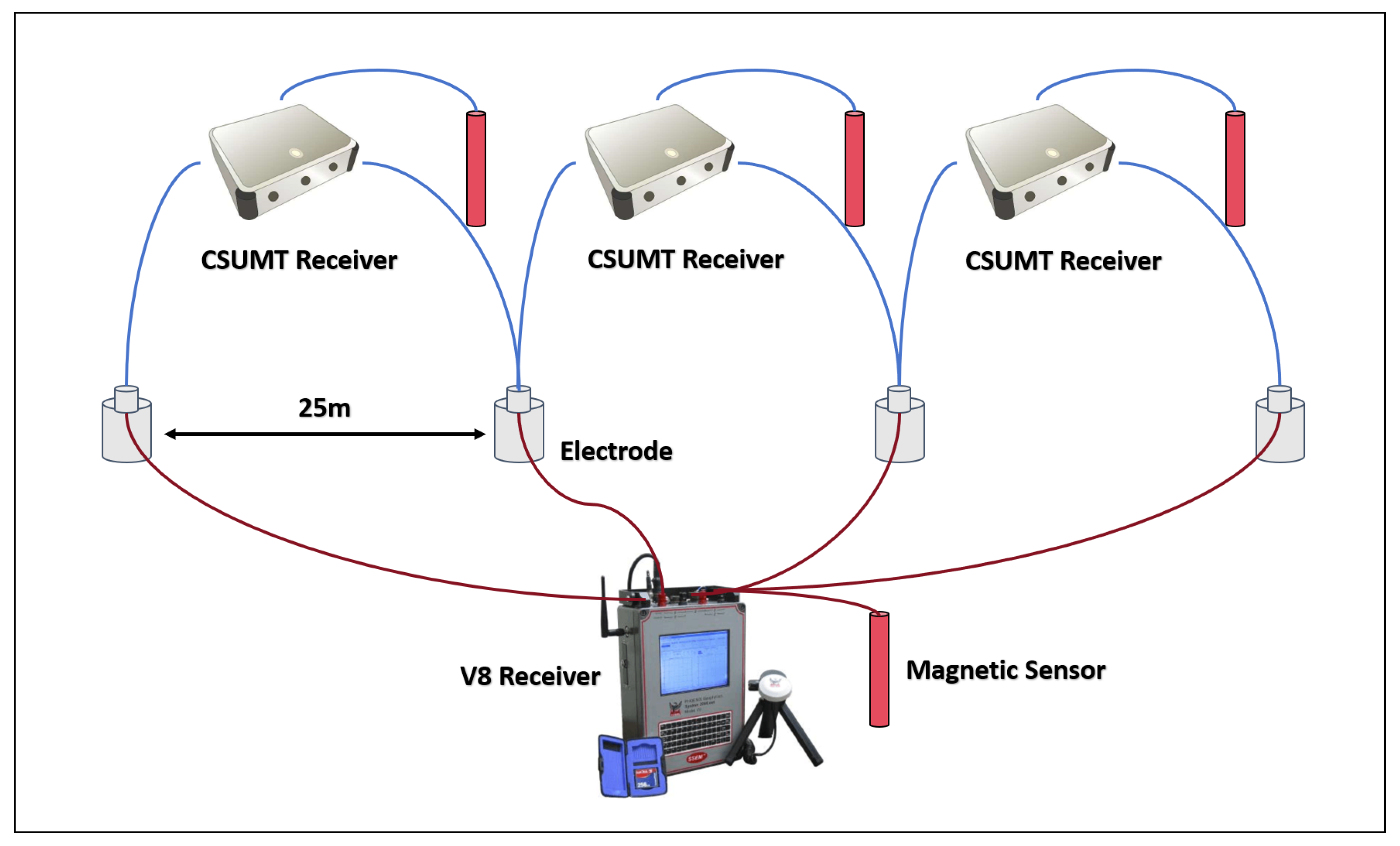
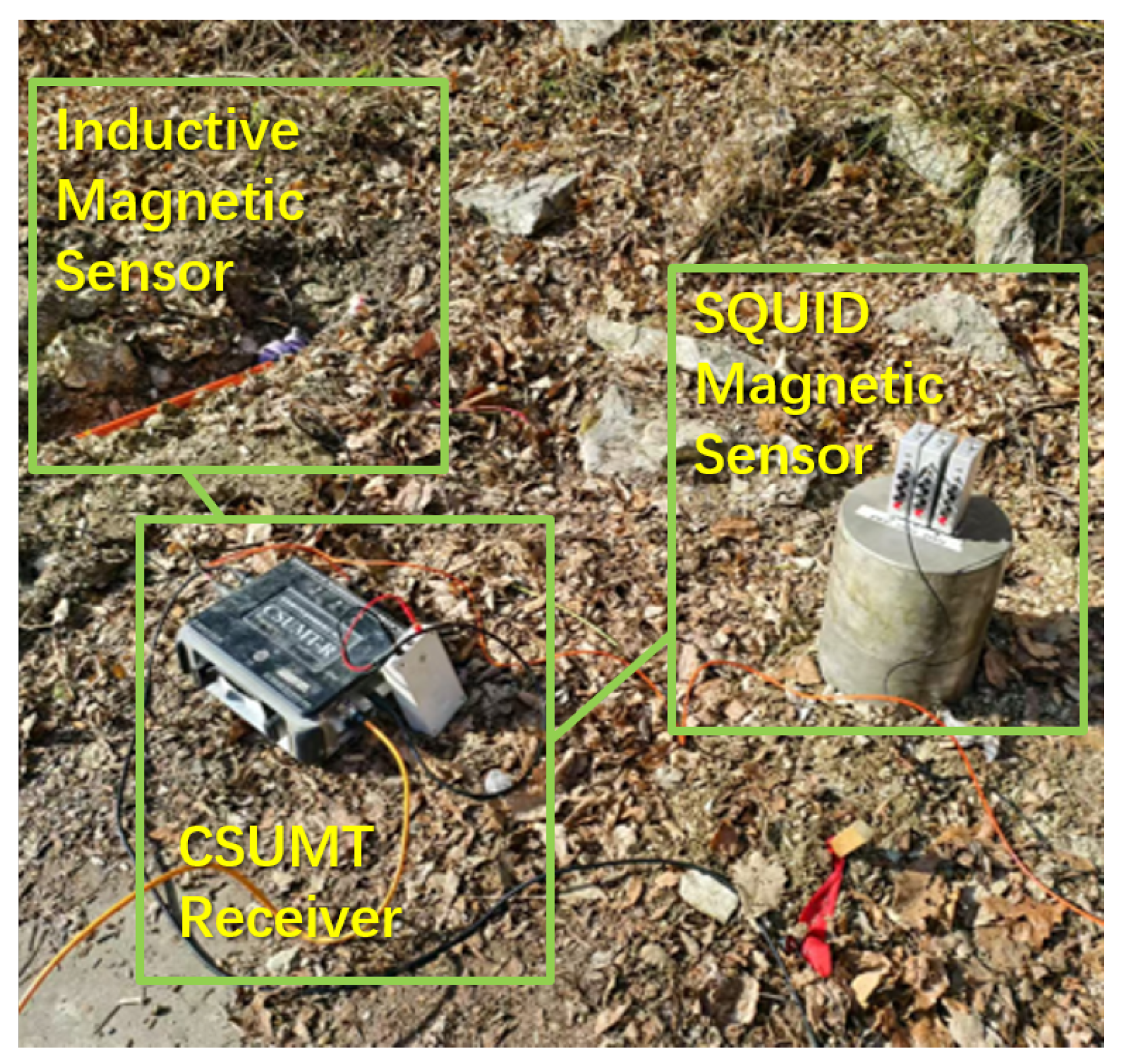
4.1. Test Design and Field Work
4.2. Test Result
5. Conclusions
Author Contributions
Funding
Institutional Review Board Statement
Informed Consent Statement
Data Availability Statement
Acknowledgments
Conflicts of Interest
References
- Tikhonov, A. On determining electric characteristics of the deep layers of the Earth’s crust. Dolk. Acad. Nauk. SSSR 1950, 73, 295–297. [Google Scholar]
- Meju, M.A. Geoelectromagnetic Exploration For Natural Resources: Models, Case Studies And Challenges. Surv. Geophys. 2002, 23, 133–206. [Google Scholar] [CrossRef]
- Goldstein, M.A. Audio-Frequency Magnetotellurics with a Grounded Electric Dipole Source. Geophysics 1975, 40, 669. [Google Scholar] [CrossRef]
- Sandberg, S.K.; Hohmann, G.W. Controlled-Source audiomagnetotellurics in geothermal exploration. Geophysics 1982, 47, 100–116. [Google Scholar] [CrossRef]
- Zonge, K.L. Controlled source audio-frequency magneto-tellurics. Electromagn. Methods Appl. Geophys. 1991, 2, 713–810. [Google Scholar]
- Guo, L. The Joint Bayesian Inversion of CSAMT and DC Data for the Jinba Gold Mine in Xinjiang Using Physical Property Priors. Minerals 2025, 15, 299. [Google Scholar] [CrossRef]
- Wang, R.; Di, Q.; Lei, D.; Fu, C.; Liang, P.; Wang, M. Three-dimensional CSAMT Forward Modeling of Potential Landslide Sliding Surfaces Using Finite Element Method. Appl. Geophys. Bull. Chin. Geophys. Soc. 2024, 21, 621–638. [Google Scholar] [CrossRef]
- He, H.; Wang, J.; Wen, W.; Tian, R.; Lin, J.; Huang, W.; Li, Y. Deep Structure of Epithermal Deposits in Youxi Area: Insights from CSAMT and Dual-Frequency IP Data. Minerals 2024, 14, 27. [Google Scholar] [CrossRef]
- Phoenix Geophysics. Ultra-wideband MT Systems. 2025. Available online: https://www.phoenixgeophysics.com/ultra-wideband-mt-systems (accessed on 10 April 2025).
- Geometrics. Stratagem EH-5. 2025. Available online: https://www.geometrics.com/product/stratagem-eh5/ (accessed on 10 April 2025).
- Zonge International. Geophysical Data Processing Receivers. 2025. Available online: http://zonge.com/instruments-home/instruments/receivers/ (accessed on 10 April 2025).
- Bastani, M.; Malehmir, A.; Ismail, N.; Pedersen, L.B.; Hedjazi, F. Delineating hydrothermal stockwork copper deposits using Controlled-Source and radio-magnetotelluric methods: A case study from northeast Iran. Geophysics 2009, 74, B167–B181. [Google Scholar] [CrossRef]
- Bastani, M.; Savvaidis, A.; Pedersen, L.B.; Kalscheuer, T. CSRMT measurements in the frequency range of 1–250kHz to map a normal fault in the Volvi basin, Greece. J. Appl. Geophys. 2011, 75, 180–195. [Google Scholar] [CrossRef]
- Saraev, A.; Simakov, A.; Shlykov, A.; Tezkan, B. Controlled source radiomagnetotellurics: A tool for near surface investigations in remote regions. J. Appl. Geophys. 2017, 146, 228–237. [Google Scholar] [CrossRef]
- Saraev, A.; Simakov, A.; Tezkan, B.; Tokarev, I.; Shlykov, A. On the study of industrial waste sites on the Karelian Isthmus/Russia using the RMT and CSRMT methods. J. Appl. Geophys. 2020, 175, 103993. [Google Scholar] [CrossRef]
- Popa, P.D.; Rezlescu, N.; Anghelache, R. Inductive sensor for slow varying magnetic fields. Sens. Actuators Phys. 1997, 59, 219–221. [Google Scholar] [CrossRef]
- Petridis, C.; Petrou, I.; Dimitropoulos, P.; Hristoforou, E. Determining Appropriate Magnetic Core Properties for a New Type of Flux-Gate Like Sensor. Sens. Lett. 2007, 5, 98–101. [Google Scholar] [CrossRef]
- Michael, P.; Julian, L.; Klaus, D.K. An ultra-low field SQUID magnetometer for measuring antiferromagnetic and weakly remanent magnetic materials at low temperatures. Rev. Sci. Instruments 2023, 94, 103904.1–103904.7. [Google Scholar]


| Parameter | V8 | Stratagem EH-5 | GDP32II | CSUMT Receiver |
|---|---|---|---|---|
| Number of channels | 6 | 5 | up to 16 | 5 |
| Frequency range | 0.00005 Hz to 10 kHz | 1 Hz to 96 kHz | 0.0007 Hz to 8 kHz | 1 Hz to 1 MHz |
| ADC | 24-bit | 32-bit | 16-bit | 24-bit |
| Size | 21.5 × 23 × 14 cm | 36 × 36 × 32 cm | 43 × 41 × 23 | 34 × 28 × 15 |
| Weight | 7 kg | 5.8 kg | 13.7 kg to 19.1 kg | 5.7 kg |
| Dynamic range | 130 dB | 127 dB | 190 dB | 135 dB @ 305 SPS |
| Frequency (Hz) | Duration (s) |
|---|---|
| 1 | 60 |
| 2 | 60 |
| 4 | 60 |
| 8 | 60 |
| 16 | 60 |
| 32 | 60 |
| 64 | 60 |
| 128 | 60 |
| 256 | 60 |
| 512 | 60 |
| 768 | 60 |
| 1024 | 60 |
| 1280 | 60 |
| 1920 | 60 |
| 2560 | 60 |
| 3840 | 60 |
| 5120 | 60 |
| 6400 | 60 |
| 7680 | 60 |
| 9600 | 60 |
| 15,800 | 18 |
| 20,013 | 18 |
| 25,128 | 18 |
| 31,588 | 18 |
| 39,766 | 18 |
| 50,155 | 18 |
| 63,015 | 18 |
| 79,277 | 18 |
| 100,721 | 18 |
| 126,680 | 18 |
| 159,584 | 18 |
| 201,442 | 18 |
| 256,000 | 18 |
| 323,368 | 18 |
| 396,387 | 18 |
| 491,520 | 18 |
| 614,400 | 18 |
| Frequency (Hz) | Inductive Magnetic Sensor | SQUID Magnetic Sensor |
|---|---|---|
| 1 | 0.06742 | 0.00197 |
| 2 | 0.00821 | 0.00049 |
| 4 | 0.00314 | 0.00022 |
| 8 | 0.00201 | 0.00042 |
| 16 | 0.00296 | 0.00335 |
| 32 | 0.00159 | 0.00095 |
| 64 | 0.00289 | 0.00316 |
| 128 | 0.00128 | 0.00121 |
| 256 | 0.00157 | 0.00154 |
| 512 | 0.00271 | 0.00248 |
| 768 | 0.00540 | 0.00710 |
| 1024 | 0.00485 | 0.00272 |
Disclaimer/Publisher’s Note: The statements, opinions and data contained in all publications are solely those of the individual author(s) and contributor(s) and not of MDPI and/or the editor(s). MDPI and/or the editor(s) disclaim responsibility for any injury to people or property resulting from any ideas, methods, instructions or products referred to in the content. |
© 2025 by the authors. Licensee MDPI, Basel, Switzerland. This article is an open access article distributed under the terms and conditions of the Creative Commons Attribution (CC BY) license (https://creativecommons.org/licenses/by/4.0/).
Share and Cite
Lin, Z.; Zhang, Q.; Zhang, R.; Zhang, X.; Zhang, H.; Wang, X.; Li, H.; Liu, Y.; Zhou, B.; Shao, J.; et al. Field Testing of a Controlled-Source Wide Frequency Range Magnetotelluric Detector Using SQUID and Inductive Magnetic Sensors. Sensors 2025, 25, 3896. https://doi.org/10.3390/s25133896
Lin Z, Zhang Q, Zhang R, Zhang X, Zhang H, Wang X, Li H, Liu Y, Zhou B, Shao J, et al. Field Testing of a Controlled-Source Wide Frequency Range Magnetotelluric Detector Using SQUID and Inductive Magnetic Sensors. Sensors. 2025; 25(13):3896. https://doi.org/10.3390/s25133896
Chicago/Turabian StyleLin, Zucan, Qisheng Zhang, Rongbo Zhang, Xiyuan Zhang, Hui Zhang, Xinchang Wang, Huiying Li, Yunheng Liu, Bojian Zhou, Jian Shao, and et al. 2025. "Field Testing of a Controlled-Source Wide Frequency Range Magnetotelluric Detector Using SQUID and Inductive Magnetic Sensors" Sensors 25, no. 13: 3896. https://doi.org/10.3390/s25133896
APA StyleLin, Z., Zhang, Q., Zhang, R., Zhang, X., Zhang, H., Wang, X., Li, H., Liu, Y., Zhou, B., Shao, J., & Zhou, K. (2025). Field Testing of a Controlled-Source Wide Frequency Range Magnetotelluric Detector Using SQUID and Inductive Magnetic Sensors. Sensors, 25(13), 3896. https://doi.org/10.3390/s25133896