

Dual-Branch Multi-Dimensional Attention Mechanism for Joint Facial Expression Detection and Classification


Abstract
1. Introduction
- Novel Application of Attention Mechanisms: While batch attention, AGCA, and NA are not novel inventions, this work represents their first deployment in simultaneous facial expression detection and classification. Specifically, we introduce (i) batch attention for this dual task, (ii) AGCA with adaptive channel weighting for FER, and (iii) NA integrated into residual networks for spatial processing in FER.
- First Integrated Architecture: The design integrating these three attention mechanisms within a dual-input stream framework, processing features through YOLOX’s head network, constitutes the first such architecture across any application domain. This model achieves state-of-the-art results on challenging non-aligned FER datasets (RAF-DB and SFEW).
- Proven Generalization Capability: The model demonstrates strong generalization to real-world scenarios, validated on unseen "in-the-wild" test data not encountered during training, confirming its practical robustness beyond benchmark datasets.
2. Related Work
2.1. Facial Expression Recognition
2.2. YOLO
2.3. Attention Mechanisms
2.4. Facial Expression Datasets
3. Method
3.1. Overview
3.2. The YOLOX Framework
3.2.1. Backbone Network
3.2.2. Neck Network
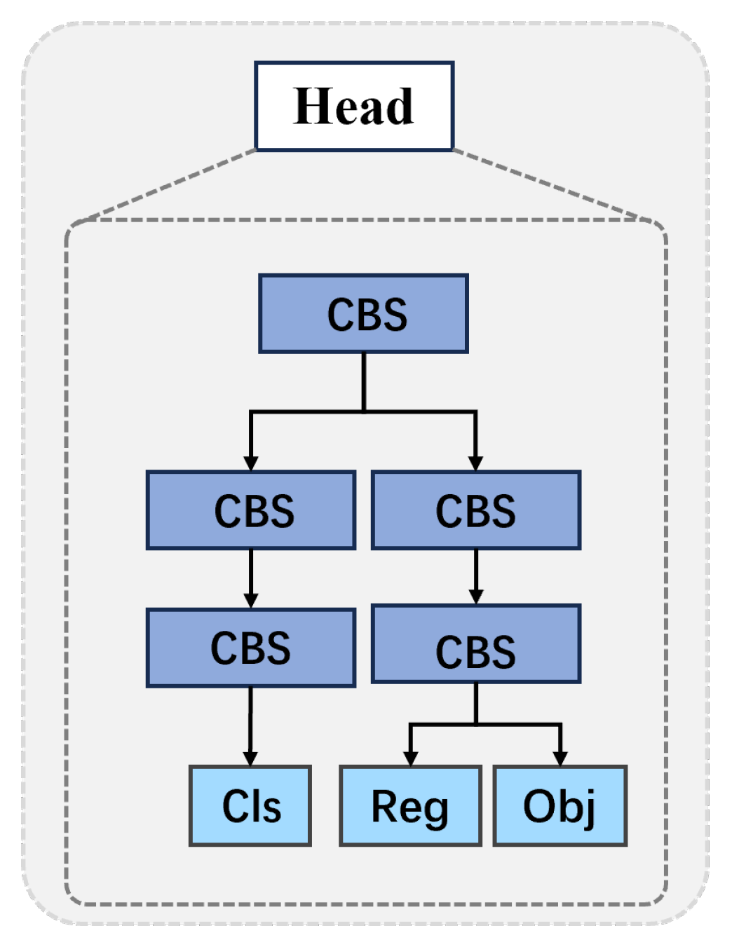
3.2.3. Head Network
3.3. Structure of the Feature Extractor
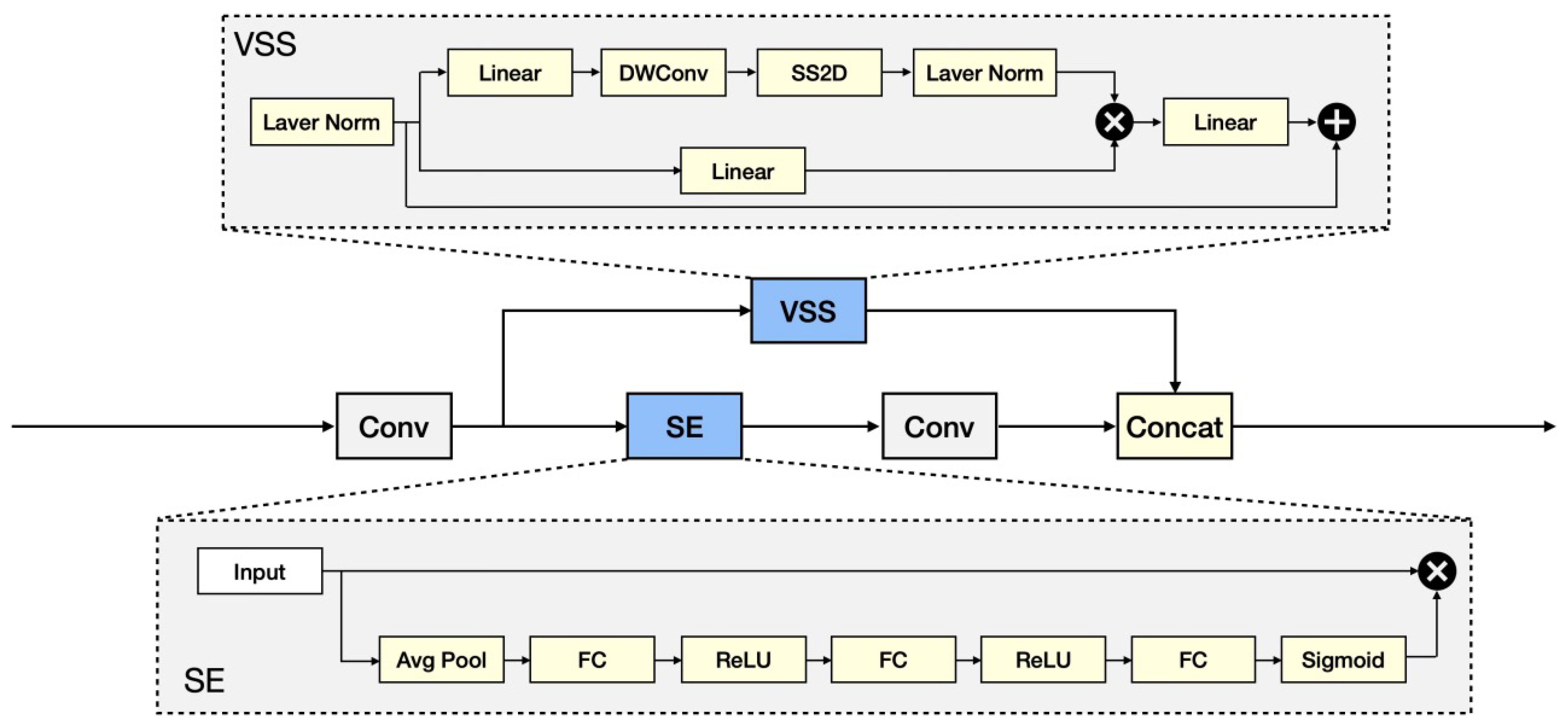
3.3.1. Pre-Conditioning Unit: Parallel Structure of VSS and SE
- VSS module
- SE Module
3.3.2. Attention Mechanism
- Self Attention [56]
- Neighborhood Attention [34]
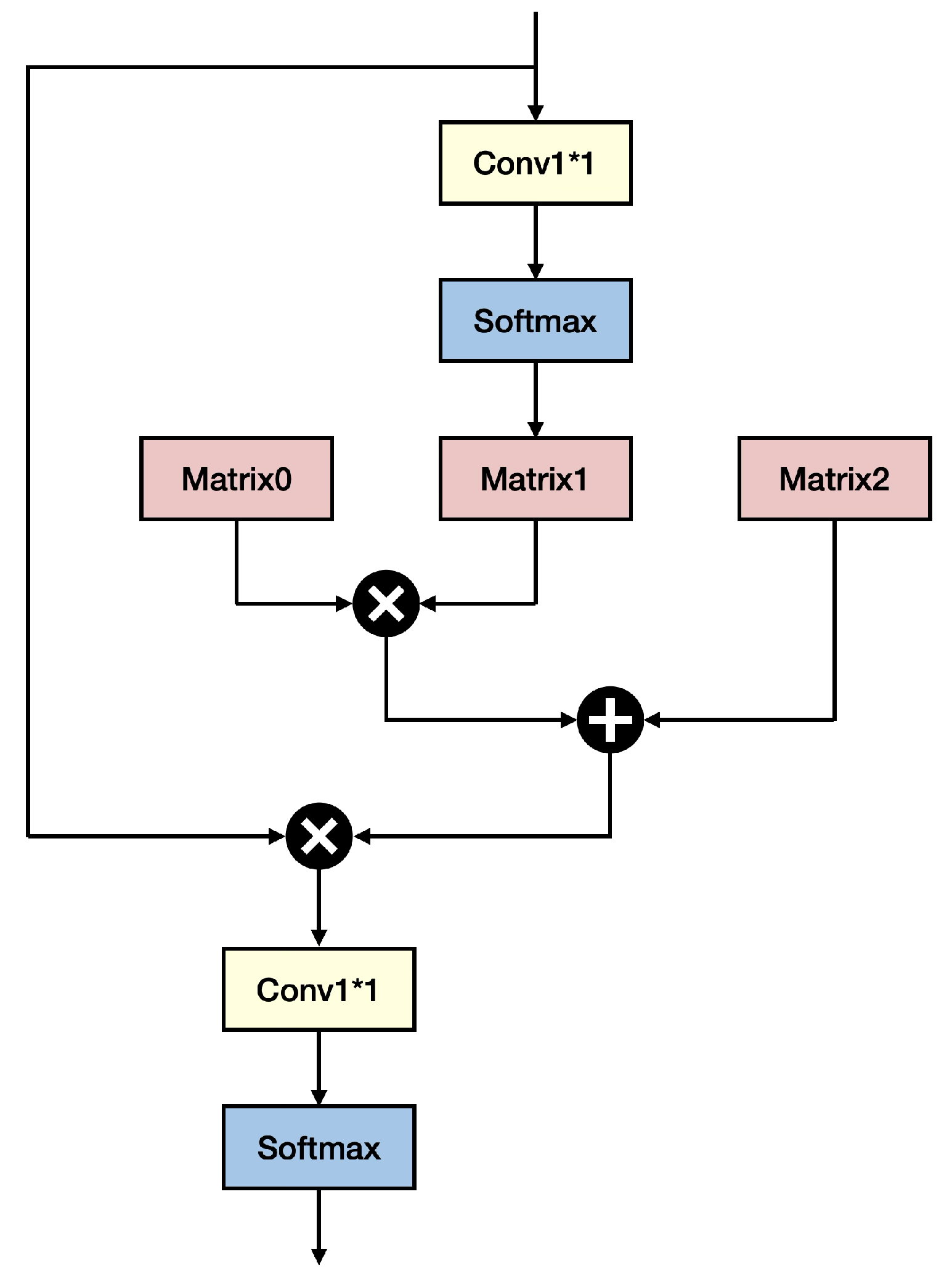
- Adaptive Graph Channel Attention [33]
3.4. The Overall Structure of the DB-MDA
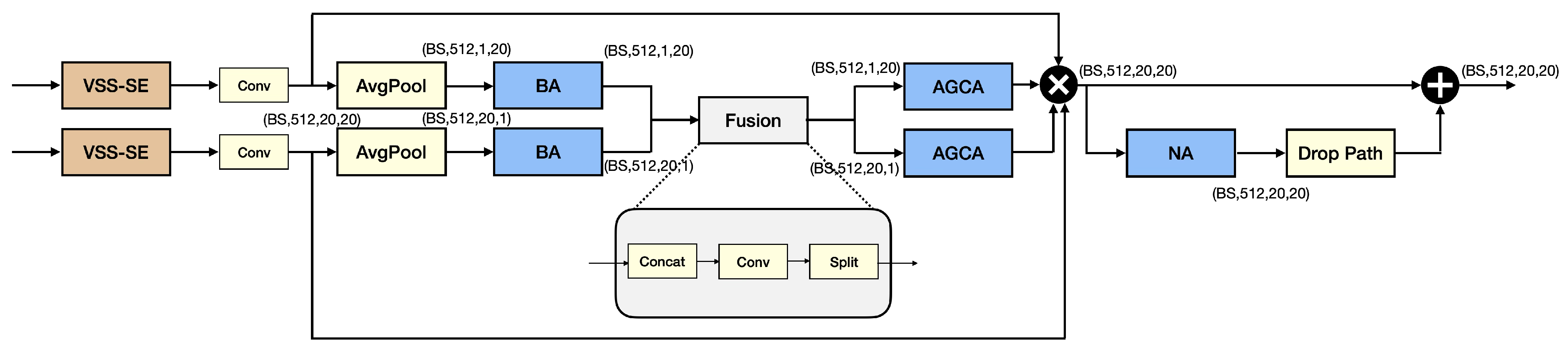
- BA-AGCA unit
- Novelty of the DB-MDA module
- Our DB-MDA model uses BA, while this is absent from that of FER-NCAMamba.
- DB-MDA does not use coordinate attention, while FER-NCAMamba uses it.
- DB-MDA deploys AGCA to extract channel weights dyanmically, one for each element of the input channels, while FER-NCAMamba uses channel attention as the final module before the output stage.
- DB-MDA uses NA in a residual network while FER-NCAMamba uses NA in a feedforward fashion together with coordinate attention.
4. Experiments
4.1. Datasets
4.1.1. RAF-DB and SFEW Datasets
- RAF-DB
- SFEW
4.1.2. Additional Images to Evaluate the Generalization Capabilities of Both Trained Models on Unseen Data
- Details of Camera Used
- Details of the images captured
4.2. Implementation Details
- Explanation of some of the terms used in Table 2
4.3. Evaluation Metrics
- Precision and Recall Calculation:where TP represents the number of true positives, FP represents the number of false positives, and FN represents the number of false negatives.It is possible to combine the precision and recall into an F1 score:
- Average Precision (AP) Calculation:Average precision is the mean of precision values at different recall levels, calculated by integrating the precision–recall curve:where denotes the precision at recall r.Likewise, it is possible to compute the average recall and the average F1 accordingly.
- Mean Average Precision (mAP) Calculation:The mean of the AP values for all N categories is calculated as follows:where N is the total number of categories and is the average precision for the i-th category.The mAP reflects the model’s detection performance across all categories and provides an evaluation of the overall detection capabilities of the model.
4.4. Ablation Experiments
- (i)
- the full module with all components in place (this corresponds to the first row in Table 3 and subsequent rows in the table followed the same convention).
- (ii)
- removing BA by itself and replaced by a direct connection,
- (iii)
- removing AGCA by itself, with the BA in place, and replaced the AGCA by a direct connection,
- (iv)
- removing both BA and AGCA, and replaced by a direct connection,
- (v)
- replace the dual branch BA, AGCA modules, and the NA module by a direct connection, with only the VSS-SE module in place,
- (vi)
- removing the dual branch BA AGCA modules, the NA module, and the VSS-SE module, and replacing with a direct connection; in other words, there is no VSS-SE module, nor any of the attention components.
- BA, AGCA, and NA play a crucial role in enhancing the model’s performance. According to the experimental results shown in Table 3, when AGCA is used alone, the mAP decreases from 83.59% to 83.11%; when BA is used alone, the mAP decreases from 83.59% to 83.39%. However, when both BA and AGCA are removed simultaneously, mAP drops to 83.27%. When BA, AGCA, and NA are removed, mAP drops to 83.00%. Therefore, it can be inferred that BA, AGCA, and NA all contribute to the model’s performance to some extent. However, it should be noted that the performance when using both AGCA and NA is worse than when using NA alone. On the other hand, the performance when using BA, AGCA, and NA together is significantly better than when using only BA and NA.Based on these observations, we hypothesize that AGCA’s effectiveness in extracting image features depends on the presence of BA. In other words, BA influences the feature extraction results of AGCA. Given the fact that AGCA is downstream from the BA in the dual branch BA-AGCA architecture, this hypothesis is a reasonable one.
- Both modules (VSS-SE and attention) contribute to improving model performance, with the attention module having the more significant impact. When the attention module is removed, the mAP drops from 83.59% to 83.00%, demonstrating its effectiveness. The VSS module also enhances the model’s performance. When the VSS-SE module is removed alongside the attention module, the mAP further decreases from 83.00% to 82.38%.
4.5. Visualization Analysis
4.6. Comparison with State-of-the-Art Methods
- It is noteworthy that, on both the SFEW and RAF-DB datasets, our method, DB-MDA, outperforms all other State-of-the-Art (SOTA) methods in terms of mAP. Specifically, on the RAF-DB dataset, our method achieves an mAP of 83.59%, while its closest competitor, FER-NCAMamba, achieves an mAP of 83.30%. On the SFEW dataset, our method attains an mAP of 69.43%, compared to FER-NCAMamba’s 68.66%. It is important to note that we used the un-aligned versions of the datasets, and therefore our results should not be compared with those obtained by methods that perform alignment on the samples before classification. In the latter case, the significance of detection would be greatly diminished. However, in such scenarios, the accuracy results may not be robust, as they are based on aligned information rather than on un-aligned samples.The superior performance of our model is attributed to our meticulously designed multi-dimensional attention mechanism. As ablation studies (see Section 4.4) have confirmed, each dimensional attention component within our multi-dimensional attention mechanism, regardless of its nature, contributes to the performance enhancement of the model—some significantly, others subtly—yet each is an indispensable force propelling our model forward.
- It is interesting to note that, in Table 4, almost all models find that “Happy” facial expression is the category that scores the best AP on both datasets. This may indicate that the expression “Happy”, because of the way it is expressed by most people by their facial muscles, is most obvious.
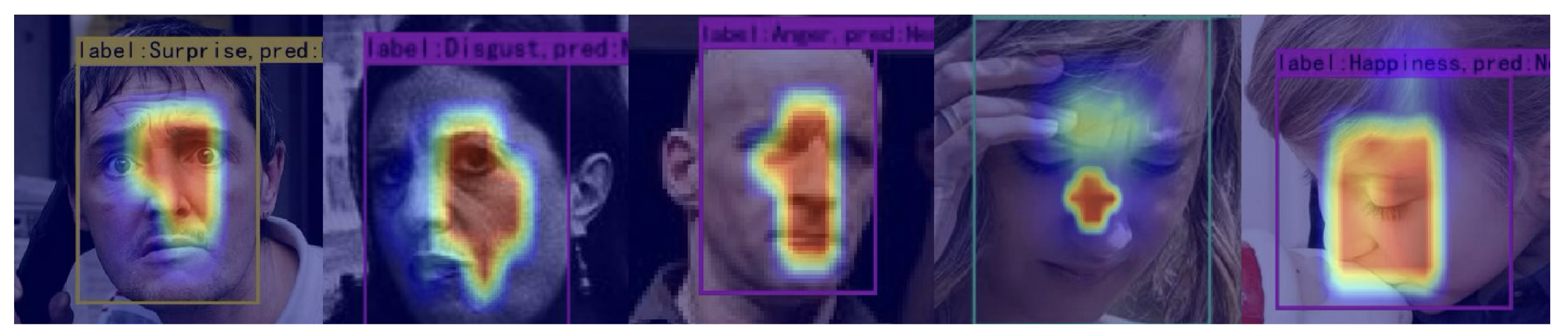
- When observing the performance of our model across different expression labels, we note that its efficacy varies with the size of the dataset. This is illustrated in Table 5.On the RAF-DB dataset, our model is better in recognizing images labeled as “Sad” and “Fear”, while its performance on other categories lags behind those of FER-NCAMamba, even though, in most cases, they are only behind in the first decimal place. This is why, on average, our model outperforms that of FER-NCAMamba, because in those two expressions, “Sad” and “Fear”, it has sufficient “head room” to provide for the overall lead. We hypothesize that, for the RAF-DB dataset, our model primarily focuses on the mouth region of the face, as the characteristics of Sad and Fear expressions are most pronounced in this area. This conjecture has been substantiated through Grad-CAM visualizations in Figure 6 and Figure 7.Similarly, our model achieves better results in identifying “Anger”, “Disgust”, “Happy”, and “Surprise” expressions on the SFEW dataset than those of the FER-NCAMamba, where the defining features of these emotions are predominantly located around the eyes, nose, and brow regions, as shown in Figure 8. Consequently, our model pays relatively more attention to these areas when processing SFEW images, a focus that has also been confirmed by Grad-CAM visualizations.These analyses shed some light on the capabilities of our model. However, these observations need to be treated with caution; there are only two datasets, and there are two methods: Ours and FER-NCAMamba. To draw more conclusive observations, one would be advised to consider more datasets, and more models rather than just two, even though these two are the ones that obtained the best and second best performances. It would be advisable to consider more models, and if possible more datasets, before making sweeping statements concerning the relationship between models and the size of datasets, even though intuitively this seems plausible. In dealing with such a challenging problem like FER from un-aligned images, where there could be labelling errors and subtle muscle movements on a face captured far from the camera, it pays to be cautious, as there could be “demons lurking around” to defy logic or common sense based on limited exposure to the data.
4.7. Evaluation of the Generalizabilities of the Trained Models on the Real Life Dataset
- In terms of accuracy, a model trained on the RAF-DB training dataset appears to be less accurate than the one trained on SFEW. Table 7 shows that the number of correctly classified images differs by only 1 (16 in the case of SFEW and 15 in the case of RAF-DB). This appears to contradict the intuition that RAF-DB has a larger number of training samples compared with that of SFEW and should provide a better recognition accuracy than that of SFEW.However, a deeper consideration of the nature between RAF-DB and SFEW and Table 7 could explain this anomaly. While the RAF-DB dataset contains un-aligned faces, it does not have the large variety of backgrounds like those occurring in the SFEW dataset. Moreover, the RAF-DB dataset contains fewer number of faces that are at a distance from the camera, while SFEW contains faces shot at considerable distance from the camera. This may explain some of the statistics as reported in Table 7. In Table 7, it is observed that the SFEW trained model makes nine instances of misclassification, while the RAF-DB trained model makes only two instances of mis-classification. This implies that RAF-DB trained model is better at correctly classifying the expression than that of a SFEW trained model. Moreover, for a SFEW trained model, it makes 11 instances of failed to recognize, while the RAF-DB trained model makes 19 instances of failed to recognize. This shows that the the RAF-DB trained model is less adept at recognizing faces shot at considerable distances from the camera, while the SFEW trained model is better adept for such occasions, as it has many more examples of such a situation occurring in its training dataset.
- Admittedly, here we have only 36 samples, and so any observations would need to be treated with caution. These can only be preliminary observations. But judging from the results of this experiment, a state-of-the-art model, like our DB-MDA model, is unlikely to be ready for deployment in real-life situations, even for relatively “lightweight’ applications like screening.
- This experiment brings to the foreground the importance of a large amount of training data with a large variety of backgrounds, and images shot with a variety of distances from the camera. However, collecting large-scale real-life data and having them labelled is expensive, and one would need a convincing use case before the expenses required could be justified. But then without convincing results from a model, it is hard to convince some institutions to invest vast sums of money without a likely good outcome in sight. This is the kind of “Catch22” situation in which researchers are caught. A good way forward would be to continuously improve on the models and slowly expand the types of data that could be used in evaluating the models to see how such models could be used on data that is more and more like real-life situations. Hopefully with enough evidence on “toy” datasets, with gradual relaxation in the direction of real-life situations, the area would be ready for commercial exploration.
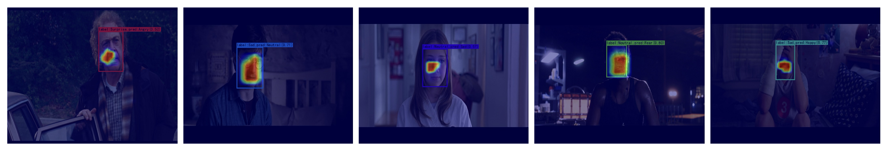
- It is observed that, despite the cluttered background in most images, both trained models appear to be able to find the bounding boxes that delimit the human faces in the image.
- While the face is correctly located, the region of the heatmap overlaid on the detected face cannot be discerned. They are often not focused on the regions in which the facial expression most likely would manifest, e.g., the corner of the mouth, the corner of the eye. Instead, sometimes it focuses on the chin, sometimes it is across the forehead, and sometimes, it is a “smudge” around the nose and mouth regions.This may point in the direction that the input image resolution used, , might not be high enough to reveal the fine details of such regions when the face is at a considerable distance from the camera. Moreover, it is observed that, where no bounding box is found (when the emotion score falls below a threshold of 0.5), the heatmap could fall on the general area for recognition.This may also point to the fact that the feature extractor designed is not sensitive enough to the fine features that are displayed in these regions. Admittedly, currently we only generate three scaled signals from the input image. It may be useful to experiment with a FPN with more scales than three. This may delineate if the issue arises due to the lack of high-resolution inputs.
4.8. Discussions on the Differences in the Capability of FER-NCAMamba and DB-MDA Models
- It is observed that the FER-NCA model and the DB-MDA model have a different balance between the undetected and the classified errors. The DB-MDA model appears to have struck a better balance between classification accuracies and un-detected errors. The DB-MDA model achieves a total number of misclassifications of 309 when compared with that of the FER-NCA model of 337, while it had 163 undetected faces and FER-NCA had 159 undetected faces.
- It appears that, for the FER-NCA model, the categories in which it made most mistakes in classification when compared with those of DB-MDA would be “Happiness” and “Neutral”, and in every other categories, except in the category of “Disgust”, it made slightly less errors than that of the DB-MDA model.
- These results show conclusively that these two models are doing different things on the RAF-DB dataset: FER-NCA makes a lesser balance on the classification and detection capacities than those of DB-MDA.
- The question of why DB-MDA achieves a better balance between classification and detection would require extensive investigations of the qualities of the features extracted by either model, especially in relation to the global features for detection and the fine features used in classification, with respect to their designs. This task would be a good topic for future work.
4.9. Limitations of Our DB-MDA Model
- Investigations reported in Section 4.7 reveals an uncomfortable truth about most deep learning methods: They works well on “toy” datasets, where the training dataset and the testing dataset are obtained in the same environment. However, if the trained model is applied to samples that are collected using different environments, then the performance degrades, sometimes dramatically. This is typified in the experiment we conducted in Section 4.7.A way forward would be to explore few shot learning (see, e.g., [70]), in which new samples collected from different environments could be incorporated through this methodology. A sideline of this research, which may be more immediate, would be to explore more sophisticated data augmentation schemes, like those used in [70]. This would increase the diversity of images, and thus would make the recognition more robust.In the longer term, there is a need to collect more data under a variety of backgrounds, a variety of distances between the subject and the camera, more than one subject in some of the images, and under various lighting conditions, and label them accordingly. The availability of large-scale FER datasets would facilitate the development of improved models.
- As shown clearly in Section 4.8, it strikes a better balance than the FER-NCA model in apportioning the conflicting demands of global features for detection purposes and fine features for good classification of facial expressions; there are still 10% misclassfied samples and 5% undetected faces in the testing dataset of RAF-DB. Depending on the application, e.g., screening, such margins of errors could be tolerable. However such error margins might not sit comfortably if this is used for diagnosis purposes. But then, if the idea of FER from static images is used together with other physiological measurements, an ensemble type of method could be used to combine the individual physiological measurements and FER and such an error margin could be tolerable. A suitably designed ensemble method would improve the accuracy in determining the emotions of the person.
- Currently, the loss function used to train the model consists of three components: the cross entropy loss, the IoU (Intersection over Union) loss for determining the location of the bounding boxes and the ground truth information, and the objectness confidence indicating the probability of object presence. These loss functions could suitably be augmented by other measures. For example, within AGCA, there is no control on the magnitude of the elements of the matrix . While every effort has been taken to condition these elements to behave well, like initializing them with very small values, and through small learning rates and high momentum terms, the very idea that some of these elements could grow without limits is uncomfortable, even though, on the two datasets used to evaluate the model, RAF-DB and SFEW, no observable growth is discerned in all experiments. It is possible to include in the loss function a regularization term, on the size of the elements of matrix , and to ensure its diagonal elements will be close to 0. This would force the elements to stay within some bound and the diagonal elements to be close to 0.
- Among the three attention mechanisms used, both the operation in the channel dimension and in the spatial dimension are currently the most sophisticated ones available; only the batch attention is still quite crude, as it uses the self-attention mechanism in the batch dimension. It is perceivable that one could use a version of neighborhood attention along the batch dimension.
- The attention mechanisms used is one way of extracting features. There are other developments in the area of feature extraction, e.g., in emphasizing the role of discriminative regression projection in feature extractions (see, e.g., [71]). Incorporating features extracted using other ideas than attention mechanism might improve the types of feature extracted for SDAC tasks. This would be a fruitful area of further research.
5. Conclusions
Author Contributions
Funding
Institutional Review Board Statement
Informed Consent Statement
Data Availability Statement
Acknowledgments
Conflicts of Interest
References
- Saganowski, S. Bringing emotion recognition out of the lab into real life: Recent advancies in sensors and machine learning. Electronics 2022, 11, 496. [Google Scholar] [CrossRef]
- Breazeal, C.; Dautenhahn, K.; Kanda, T. Social robotics. In Springer Handbook of Robotics; Springer: Cham, Switzerland, 2016; pp. 1935–1972. [Google Scholar]
- Kumar, A.; Kumar, A.; Jayakody, D.N.K. Ambiguous facial expression detection for Autism Screening using enhanced YOLOv7-tiny model. Sci. Rep. 2024, 14, 28501. [Google Scholar] [CrossRef] [PubMed]
- Zeng, Z.; Pantic, M.; Roisman, G.I.; Huang, T.S. A survey of affect recognition methods: Audio, visual and spontaneous expressions. In Proceedings of the 9th International Conference on Multimodal Interfaces, Nagoya, Japan, 12–15 November 2007; pp. 126–133. [Google Scholar]
- Sikander, G.; Anwar, S. Driver fatigue detection systems: A review. IEEE Trans. Intell. Transp. Syst. 2018, 20, 2339–2352. [Google Scholar] [CrossRef]
- Zhan, C.; Li, W.; Ogunbona, P.; Safaei, F. A real-time facial expression recognition system for online games. Int. J. Comput. Games Technol. 2008, 2008, 542918. [Google Scholar] [CrossRef]
- Akbara, M.T.; Ilmia, M.N.; Rumayara, I.V.; Moniagaa, J.; Chenb, T.K.; Chowandaa, A. Enhancing Game Experience with Facial Expression Recognition as Dynamic Balancing. Procedia Comput. Sci. 2019, 157, 388–395. [Google Scholar] [CrossRef]
- Gross, J.; Feldman Barrett, L. Emotion generation and emotion regulation: One or two depends on your point of view. Emotion. Rev. 2011, 3, 8–16. [Google Scholar] [CrossRef] [PubMed]
- Damasio, A.R. The Feeling of What Happens: Body and Emotion in the Making of Consciousness; Mariner Books: Boston, MA, USA, 1999. [Google Scholar]
- Rosenberg, E.L.; Ekman, P.E. What the Face Reveals: Basic and Applied Studies of Spontaneous Expression Using the Facial Action Coding System (FACS); Oxford University Press: Oxford, UK, 1997. [Google Scholar]
- Plutchik, R. A general psychoevolutionary theory of emotion. In Theories of Emotion; Elsevier: Amsterdam, The Netherlands, 1980. [Google Scholar]
- Frijda, N. The Emotions; Cambridge University Press: Cambridge, UK, 1986. [Google Scholar]
- Gross, J. Emotion regulation: Current status and future prospects. Psychol. Sci. 2015, 26, 1–26. [Google Scholar] [CrossRef]
- Barrett, L. The future of psychology: Connecting mind to brain. Perspect. Psychol. Sci. 2009, 4, 326–339. [Google Scholar] [CrossRef]
- Mesquita, B.; Boiger, M. Emotions in context: A sociodynamic model of emotions. Emot. Rev. 2014, 6, 298–302. [Google Scholar] [CrossRef]
- Saganowski, S.; Miszczyk, J.; Kunc, D.; Lisouski, D.; Kazienko, P. Lessons Learned from Developing Emotion Recognition System for Everyday Life. In Proceedings of the SenSys: Proceedings of the 20th ACM Conference on Embedded Networked Sensor Systems, Istanbul, Turkey, 12–17 November 2023; pp. 1047–1054. [Google Scholar] [CrossRef]
- Shehu, H.A.; Browne, W.N.; Eisenbarth, H. Emotion categorization from facial expressions: A review of datasets, methods, and research directions. Neurocomputing 2025, 624, 129367. [Google Scholar] [CrossRef]
- Lucey, P.; Cohn, J.F.; Kanade, T.; Saragih, J.; Ambadar, Z.; Matthews, I. The Extended Cohn-Kanade Dataset (CK+): A complete dataset for action unit and emotion-specified expression. In Proceedings of the 2010 IEEE Computer Society Conference on Computer Vision and Pattern Recognition—Workshops, San Francisco, CA, USA, 13–18 June 2010; pp. 94–101. [Google Scholar] [CrossRef]
- Peng, C.; Li, B.; Zou, K.; Zhang, B.; Dai, G.; Tsoi, A.C. An Innovative Neighbor Attention Mechanism Based on Coordinates for the Recognition of Facial Expressions. Sensors 2024, 24, 7404. [Google Scholar] [CrossRef] [PubMed]
- Mollahosseini, A.; Hasani, B.; Mahoor, M.H. AffectNet: A Database for Facial Expression, Valence, and Arousal Computing in the Wild. IEEE Trans. Affect. Comput. 2017, 10, 18–31. [Google Scholar] [CrossRef]
- Li, S.; Deng, W.; Du, J. Reliable crowdsourcing and deep locality-preserving learning for expression recognition in the wild. In Proceedings of the IEEE Conference on Computer Vision and Pattern Recognition, Honolulu, HI, USA, 21–26 July 2017; pp. 2852–2861. [Google Scholar]
- Redmon, J. Yolov3: An incremental improvement. arXiv 2018, arXiv:1804.02767. [Google Scholar]
- Bochkovskiy, A.; Wang, C.Y.; Liao, H.Y.M. Yolov4: Optimal speed and accuracy of object detection. arXiv 2020, arXiv:2004.10934. [Google Scholar]
- Jocher, G. Ultralytics YOLOv5. 2020. Available online: https://github.com/ultralytics/yolov5 (accessed on 1 March 2024).
- Ge, Z. Yolox: Exceeding yolo series in 2021. arXiv 2021, arXiv:2107.08430. [Google Scholar]
- Wang, C.Y.; Bochkovskiy, A.; Liao, H.Y.M. YOLOv7: Trainable bag-of-freebies sets new state-of-the-art for real-time object detectors. In Proceedings of the IEEE/CVF Conference on Computer Vision and Pattern Recognition, Vancouver, BC, Canada, 17–24 June 2023; pp. 7464–7475. [Google Scholar]
- Ultralytics. YOLOv8 Documentation. 2023. Available online: https://docs.ultralytics.com/ (accessed on 1 March 2024).
- Wang, C.Y.; Liao, H.Y.M.; Wu, Y.H.; Chen, P.Y.; Hsieh, J.W.; Yeh, I.H. YOLOv10: Real-Time End-to-End Object Detection. arXiv 2024, arXiv:2405.14458. [Google Scholar]
- Ma, H.; Lei, S.; Celik, T.; Li, H.C. FER-YOLO-Mamba: Facial Expression Detection and Classification Based on Selective State Space. arXiv 2024, arXiv:2405.01828. [Google Scholar]
- Peng, C.; Sun, M.; Zou, K.; Zhang, B.; Dai, G.; Tsoi, A.C. Facial Expression Recognition-You Only Look Once-Neighborhood Coordinate Attention Mamba: Facial Expression Detection and Classification Based on Neighbor and Coordinates Attention Mechanism. Sensors 2024, 24, 6912. [Google Scholar] [CrossRef]
- Hou, Z.; Yu, B.; Tao, D. Batchformer: Learning to explore sample relationships for robust representation learning. In Proceedings of the IEEE/CVF Conference on Computer Vision and Pattern Recognition, New Orleans, LA, USA, 18–24 June 2022; pp. 7256–7266. [Google Scholar]
- Hou, Z.; Yu, B.; Wang, C.; Zhan, Y.; Tao, D. Learning to Explore Sample Relationships. IEEE Trans. Pattern Anal. Mach. Intell. 2025, 47, 5445–5459. [Google Scholar] [CrossRef]
- Xiang, X.; Wang, Z.; Zhang, J.; Xia, Y.; Chen, P.; Wang, B. AGCA: An adaptive graph channel attention module for steel surface defect detection. IEEE Trans. Instrum. Meas. 2023, 72, 1–12. [Google Scholar] [CrossRef]
- Hassani, A.; Walton, S.; Li, J.; Li, S.; Shi, H. Neighborhood attention transformer. In Proceedings of the IEEE/CVF Conference on Computer Vision and Pattern Recognition, Vancouver, BC, Canada, 17–24 June 2023; pp. 6185–6194. [Google Scholar]
- Hu, J.; Shen, L.; Albanie, S.; Sun, G.; Wu, E. Squeeze-and-Excitation Networks. In Proceedings of the 2018 IEEE/CVF Conference on Computer Vision and Pattern Recognition, Salt Lake City, UT, USA, 18–23 June 2018; pp. 7132–7141. [Google Scholar] [CrossRef]
- Wang, Q.; Wu, B.; Zhu, P.; Li, P.; Zuo, W.; Hu, Q. ECA-Net: Efficient Channel Attention for Deep Convolutional Neural Networks. In Proceedings of the IEEE Conference on Computer Vision and Pattern Recognition (CVPR), Seattle, WA, USA, 14–19 June 2020. [Google Scholar]
- Dhall, A.; Goecke, R.; Lucey, S.; Gedeon, T. Static facial expression analysis in tough conditions: Data, evaluation protocol and benchmark. In Proceedings of the 2011 IEEE International Conference on Computer Vision Workshops (ICCV workshops), Barcelona, Spain, 6–13 November 2011; pp. 2106–2112. [Google Scholar]
- Li, S.; Deng, W. Deep facial expression recognition: A survey. IEEE Trans. Affect. Comput. 2020, 13, 1195–1215. [Google Scholar] [CrossRef]
- Redmon, J. You only look once: Unified, real-time object detection. In Proceedings of the IEEE Conference on Computer Vision and Pattern Recognition, Las Vegas, NV, USA, 27–30 June 2016. [Google Scholar]
- Niu, Z.; Zhong, G.; Yu, H. A review on the attention mechanism of deep learning. Neurocomputing 2021, 452, 48–62. [Google Scholar] [CrossRef]
- Lin, L.; Peng, C.; Zhang, B.; Zou, K.; Huang, P. Cross Direction Attention Network for Facial Expression Recognition. In Proceedings of the 2023 11th International Conference on Information Systems and Computing Technology (ISCTech), Qingdao, China, 30 July–1 August 2023; pp. 181–185. [Google Scholar]
- Li, G.; Peng, C.; Zou, K.; Zhang, B. Adaptive Fusion Attention Network for Facial Expression Recognition. In Proceedings of the 2023 12th International Conference on Computing and Pattern Recognition, Qingdao, China, 27–29 October 2023; pp. 260–264. [Google Scholar]
- Dalal, N.; Triggs, B. Histograms of oriented gradients for human detection. In Proceedings of the 2005 IEEE Computer Society Conference on Computer Vision and Pattern Recognition (CVPR’05), San Diego, CA, USA, 20–25 June 2005; Volume 1, pp. 886–893. [Google Scholar]
- Pers, J.; Sulic, V.; Kristan, M.; Perse, M.; Polanec, K.; Kovacic, S. Histograms of optical flow for efficient representation of body motion. Pattern Recognit. Lett. 2010, 31, 1369–1376. [Google Scholar] [CrossRef]
- Ojala, T.; Pietikainen, M.; Maenpaa, T. Multiresolution gray-scale and rotation invariant texture classification with local binary patterns. IEEE Trans. Pattern Anal. Mach. Intell. 2002, 24, 971–987. [Google Scholar] [CrossRef]
- Zhao, G.; Pietikainen, M. Dynamic texture recognition using local binary patterns with an application to facial expressions. IEEE Trans. Pattern Anal. Mach. Intell. 2007, 29, 915–928. [Google Scholar] [CrossRef]
- Ahmed, F.; Kabir, M.H. Facial feature representation with directional ternary pattern (DTP): Application to gender classification. In Proceedings of the 2012 IEEE 13th International Conference on Information Reuse & Integration (IRI), Las Vegas, NV, USA, 8–10 August 2012; pp. 159–164. [Google Scholar]
- Ryu, B.; Rivera, A.R.; Kim, J.; Chae, O. Local directional ternary pattern for facial expression recognition. IEEE Trans. Image Process. 2017, 26, 6006–6018. [Google Scholar] [CrossRef]
- Simonyan, K.; Zisserman, A. Very Deep Convolutional Networks for Large-Scale Image Recognition. In Proceedings of the International Conference on Learning Representations, San Diego, CA, USA, 7–9 May 2015. [Google Scholar]
- Tammina, S. Transfer learning using vgg-16 with deep convolutional neural network for classifying images. Int. J. Sci. Res. Publ. (IJSRP) 2019, 9, 143–150. [Google Scholar] [CrossRef]
- Targ, S.; Almeida, D.; Lyman, K. Resnet in resnet: Generalizing residual architectures. arXiv 2016, arXiv:1603.08029. [Google Scholar]
- Zhang, B.; Ma, J.; Fu, X.; Dai, G. Logic Augmented Multi-Decision Fusion framework for stance detection on social media. Inf. Fusion 2025, 122, 103214. [Google Scholar] [CrossRef]
- Dai, G.; Yi, W.; Cao, J.; Gong, Z.; Fu, X.; Zhang, B. CRRL: Contrastive Region Relevance Learning Framework for cross-city traffic prediction. Inf. Fusion 2025, 122, 103215. [Google Scholar] [CrossRef]
- Peng, C.; Li, G.D.; Zou, K.; Zhang, B.W.; Lo, S.L.; Tsoi, A.C. SFRA: Spatial fusion regression augmentation network for facial landmark detection. Multimed. Syst. 2024, 30, 300. [Google Scholar] [CrossRef]
- Lin, T.Y.; Dollár, P.; Girshick, R.; He, K.; Hariharan, B.; Belongie, S. Feature pyramid networks for object detection. In Proceedings of the IEEE Conference on Computer Vision and Pattern Recognition, Honolulu, HI, USA, 21–26 July 2017; pp. 2117–2125. [Google Scholar]
- Vaswani, A. Attention is all you need. In Proceedings of the Advances in Neural Information Processing Systems, Long Beach, CA, USA, 4–9 December 2017. [Google Scholar]
- Huang, Z.; Zhu, Y.; Li, H.; Yang, D. Dynamic facial expression recognition based on spatial key-points optimized region feature fusion and temporal self-attention. Eng. Appl. Artifical Intell. 2024, 133, 108535. [Google Scholar] [CrossRef]
- Redmon, J.; Farhadi, A. YOLO9000: Better, faster, stronger. In Proceedings of the IEEE Conference on Computer Vision and Pattern Recognition, Honolulu, HI, USA, 21–26 July 2017; pp. 7263–7271. [Google Scholar]
- Bharati, P.; Pramanik, A. Deep learning techniques—R-CNN to mask R-CNN: A survey. In Computational Intelligence in Pattern Recognition: Proceedings of CIPR 2019; Springer: Singapore, 2020; pp. 657–668. [Google Scholar]
- Wang, C.Y.; Liao, H.Y.M.; Wu, Y.H.; Chen, P.Y.; Hsieh, J.W.; Yeh, I.H. CSPNet: A new backbone that can enhance learning capability of CNN. In Proceedings of the IEEE/CVF Conference on Computer Vision and Pattern Recognition Workshops, Seattle, WA, USA, 14–19 June 2020; pp. 390–391. [Google Scholar]
- Aguilera, A.; Mellado, D.; Rojas, F. An assessment of in-the-wild datasets for multimodal emotion recognition. Sensors 2023, 23, 5184. [Google Scholar] [CrossRef] [PubMed]
- Gu, A.; Dao, T. Mamba: Linear-time sequence modeling with selective state spaces. arXiv 2023, arXiv:2312.00752. [Google Scholar]
- Liu, Y.; Tian, Y.; Zhao, Y.; Yu, H.; Xie, L.; Wang, Y.; Ye, Q.; Jiao, J.; Liu, Y. VMamba: Visual State Space Model. arXiv 2024, arXiv:2401.10166. [Google Scholar]
- Lin, T.Y.; Maire, M.; Belongie, S.; Hays, J.; Perona, P.; Ramanan, D.; Dollár, P.; Zitnick, C.L. Microsoft coco: Common objects in context. In Proceedings of the Computer Vision–ECCV 2014: 13th European Conference, Zurich, Switzerland, 6–12 September 2014; Proceedings, Part V 13. Springer: Berlin/Heidelberg, Germany, 2014; pp. 740–755. [Google Scholar]
- Selvaraju, R.R.; Cogswell, M.; Das, A.; Vedantam, R.; Parikh, D.; Batra, D. Grad-cam: Visual explanations from deep networks via gradient-based localization. In Proceedings of the IEEE International Conference on Computer Vision, Venice, Italy, 22–29 October 2017; pp. 618–626. [Google Scholar]
- Liu, W.; Anguelov, D.; Erhan, D.; Szegedy, C.; Reed, S.; Fu, C.Y.; Berg, A.C. Ssd: Single shot multibox detector. In Proceedings of the Computer Vision–ECCV 2016: 14th European Conference, Amsterdam, The Netherlands, 11–14 October 2016; Proceedings, Part I 14. Springer: Berlin/Heidelberg, Germany, 2016; pp. 21–37. [Google Scholar]
- Ross, T.Y.; Dollár, G. Focal loss for dense object detection. In Proceedings of the IEEE Conference on Computer Vision and Pattern Recognition, Honolulu, HI, USA, 21–26 July 2017; pp. 2980–2988. [Google Scholar]
- Zhou, X.; Wang, D.; Krähenbühl, P. Objects as points. arXiv 2019, arXiv:1904.07850. [Google Scholar]
- Tan, M.; Le, Q. Efficientnet: Rethinking model scaling for convolutional neural networks. In Proceedings of the International Conference on Machine Learning, PMLR, Long Beach, CA, USA, 9–15 June 2019; pp. 6105–6114. [Google Scholar]
- Lao, C.X.; Tsoi, A.C.; Bugiolacchi, R. ConvNeXt-ECA: An Effective Encoder Network for Few-shot Learning. IEEE Access 2024, 12, 133648–133669. [Google Scholar] [CrossRef]
- Liu, Z.; Vasilakos, A.V.; Chen, X.; Zhao, Q.; Camacho, D. Discriminative approximate regression projection for feature extraction. Inf. Fusion 2025, 120, 103088. [Google Scholar] [CrossRef]


| Datasets | Train Size | Test Size | Classes |
|---|---|---|---|
| RAF-DB [21] | 12,271 | 3068 | 7 |
| SFEW [37] | 1125 | 126 | 7 |
| Category | Parameter | Value |
|---|---|---|
| Training | Input Shape | (320, 320, 3) |
| Freeze Batch Size | 16 | |
| Unfreeze Batch Size(RAF-DB) | 100 | |
| Unfreeze Batch Size(SFEW) | 50 | |
| Init Epoch | 0 | |
| Freeze Epoch | 0 | |
| Unfreeze Epoch | 300 | |
| Init Learning Rate | 0.001 | |
| Min Learning Rate | ||
| Optimizer | Adam | |
| Momentum | 0.937 | |
| Learning Rate Decay Type | cosine | |
| Post-processing | Confidence Threshold | 0.5 |
| NMS Threshold | 0.3 |
| Methods | Components | mAP (%) | Avg_F1 | Avg_Recall (%) | Avg_Precision (%) | |||
|---|---|---|---|---|---|---|---|---|
| VSS-SE | BA | AGCA | NA | |||||
| RAF-DB | ✓ | ✓ | ✓ | ✓ | 83.59 | 0.78 | 76.48 | 80.00 |
| ✓ | → | ✓ | ✓ | 82.80 | 0.78 | 75.67 | 79.84 | |
| ✓ | ✓ | → | ✓ | 83.39 | 0.78 | 76.11 | 79.83 | |
| ✓ | → | → | ✓ | 83.27 | 0.78 | 76.10 | 80.76 | |
| ✓ | → | → | → | 83.00 | 0.79 | 76.31 | 81.00 | |
| → | → | → | → | 82.38 | 0.77 | 76.01 | 78.31 | |
| Methods | Year | mAP(%) | Best AP(%) | ||
|---|---|---|---|---|---|
| SFEW | RAF-DB | SFEW | RAF-DB | ||
| SSD [66] | 2015 | 59.22 | 77.89 | 91.20 (Happy) | 95.72 (Happy) |
| RetinaNet [67] | 2017 | 56.67 | 75.63 | 81.87 (Happy) | 94.63 (Happy) |
| YOLOv3 [22] | 2018 | 19.18 | 59.42 | 50.28 (Happy) | 88.09 (Happy) |
| CenterNet [68] | 2019 | 28.48 | 59.92 | 68.57 (Happy) | 91.32 (Happy) |
| EfficientNet [69] | 2019 | 15.87 | 71.45 | 29.68 (Happy) | 93.75 (Happy) |
| YOLOv4 [23] | 2020 | 12.31 | 42.23 | 29.58 (Anger) | 87.61 (Happy) |
| YOLOv5 [24] | 2020 | 13.63 | 50.15 | 25.52 (Neutral) | 91.77 (Happy) |
| YOLOvX [25] | 2021 | 64.02 | 78.40 | 90.81 (Happy) | 96.82 (Happy) |
| YOLOv7 [26] | 2022 | 52.02 | 68.17 | 74.34 (Happy) | 92.01 (Happy) |
| YOLOv8 [27] | 2023 | 51.94 | 72.09 | 87.50 (Happy) | 93.33 (Happy) |
| YOLOv10 [28] | 2024 | 64.81 | 79.58 | 88.61 (Happy) | 94.18 (Happy) |
| FER-YOLO-Mamba [29] | 2024 | 66.67 | 80.31 | 90.94 (Happy) | 97.43 (Happy) |
| FER-NCAMamba [30] | 2024 | 68.66 | 83.30 | 86.50 (Happy) | 95.31 (Happy) |
| Ours | - | 69.43 | 83.59 | 91.26 (Happy) | 95.16 (Happy) |
| Expression | SFEW | RAF-DB | ||
|---|---|---|---|---|
| Ours | FER-NCAMamba [30] | Ours | FER-NCAMamba [30] | |
| Anger | 76.29 | 75.75 | 84.27 | 85.82 |
| Disgust | 79.22 | 75.25 | 63.01 | 63.24 |
| Fear | 55.68 | 61.56 | 69.11 | 67.32 |
| Happy | 91.26 | 86.50 | 95.16 | 95.31 |
| Neutral | 46.41 | 59.38 | 90.74 | 90.92 |
| Sad | 69.36 | 66.03 | 90.16 | 88.99 |
| Surprise | 67.78 | 56.16 | 91.37 | 91.46 |
| Average | 69.43 | 68.66 | 83.59 | 83.30 |
| Model | RAF_DB | SFEW |
|---|---|---|
| Accuracy | 41.67 | 44.45 |
| mAP | 45.45 1 | 45.45 2 |
| Dataset | Correctly Classified | Failed to Recognize | Misclassified | Total |
|---|---|---|---|---|
| RAF-DB | 15 | 19 | 2 | 36 |
| SFEW | 16 | 11 | 9 | 36 |
| True Label | Predicted Class | Undetected | |||||||
|---|---|---|---|---|---|---|---|---|---|
| Anger | Disgust | Fear | Happiness | Neutral | Sadness | Surprise | Total | ||
| Anger | – | 9 | 3 | 4 | 8 | 3 | 1 | 28 | 13 |
| Disgust | 4 | – | 0 | 15 | 22 | 12 | 1 | 54 | 22 |
| Fear | 1 | 0 | – | 4 | 3 | 9 | 8 | 25 | 7 |
| Happiness | 3 | 9 | 1 | – | 26 | 8 | 5 | 52 | 38 |
| Neutral | 0 | 8 | 0 | 18 | – | 46 | 11 | 83 | 38 |
| Sadness | 1 | 8 | 0 | 8 | 39 | – | 3 | 59 | 19 |
| Surprise | 3 | 2 | 3 | 7 | 15 | 6 | – | 36 | 22 |
| Total | 12 | 36 | 7 | 56 | 113 | 84 | 29 | 337 | 159 |
| True Label | Predicted Class | Undetected | |||||||
|---|---|---|---|---|---|---|---|---|---|
| Anger | Disgust | Fear | Happiness | Neutral | Sadness | Surprise | Total | ||
| Anger | – | 6 | 2 | 5 | 9 | 1 | 0 | 23 | 16 |
| Disgust | 8 | – | 0 | 9 | 25 | 15 | 2 | 59 | 17 |
| Fear | 2 | 1 | – | 3 | 4 | 6 | 8 | 24 | 5 |
| Happiness | 4 | 6 | 0 | – | 24 | 5 | 4 | 43 | 42 |
| Neutral | 2 | 10 | 0 | 17 | – | 40 | 6 | 75 | 34 |
| Sadness | 4 | 7 | 2 | 7 | 34 | – | 0 | 54 | 24 |
| Surprise | 3 | 2 | 6 | 3 | 13 | 4 | – | 31 | 25 |
| Total | 23 | 32 | 10 | 44 | 109 | 71 | 20 | 309 | 163 |
Disclaimer/Publisher’s Note: The statements, opinions and data contained in all publications are solely those of the individual author(s) and contributor(s) and not of MDPI and/or the editor(s). MDPI and/or the editor(s) disclaim responsibility for any injury to people or property resulting from any ideas, methods, instructions or products referred to in the content. |
© 2025 by the authors. Licensee MDPI, Basel, Switzerland. This article is an open access article distributed under the terms and conditions of the Creative Commons Attribution (CC BY) license (https://creativecommons.org/licenses/by/4.0/).
Share and Cite
Peng, C.; Li, B.; Zou, K.; Zhang, B.; Dai, G.; Tsoi, A.C. Dual-Branch Multi-Dimensional Attention Mechanism for Joint Facial Expression Detection and Classification. Sensors 2025, 25, 3815. https://doi.org/10.3390/s25123815
Peng C, Li B, Zou K, Zhang B, Dai G, Tsoi AC. Dual-Branch Multi-Dimensional Attention Mechanism for Joint Facial Expression Detection and Classification. Sensors. 2025; 25(12):3815. https://doi.org/10.3390/s25123815
Chicago/Turabian StylePeng, Cheng, Bohao Li, Kun Zou, Bowen Zhang, Genan Dai, and Ah Chung Tsoi. 2025. "Dual-Branch Multi-Dimensional Attention Mechanism for Joint Facial Expression Detection and Classification" Sensors 25, no. 12: 3815. https://doi.org/10.3390/s25123815
APA StylePeng, C., Li, B., Zou, K., Zhang, B., Dai, G., & Tsoi, A. C. (2025). Dual-Branch Multi-Dimensional Attention Mechanism for Joint Facial Expression Detection and Classification. Sensors, 25(12), 3815. https://doi.org/10.3390/s25123815