
Quality Assessment of High-Speed Motion Blur Images for Mobile Automated Tunnel Inspection


Abstract
1. Introduction
2. Related Research
2.1. Camera-Based Tunnel Scanning Systems for Automation in Inspection
2.2. IQA for Motion Blur
3. Methodology
3.1. Modulation Transfer Function (MTF)
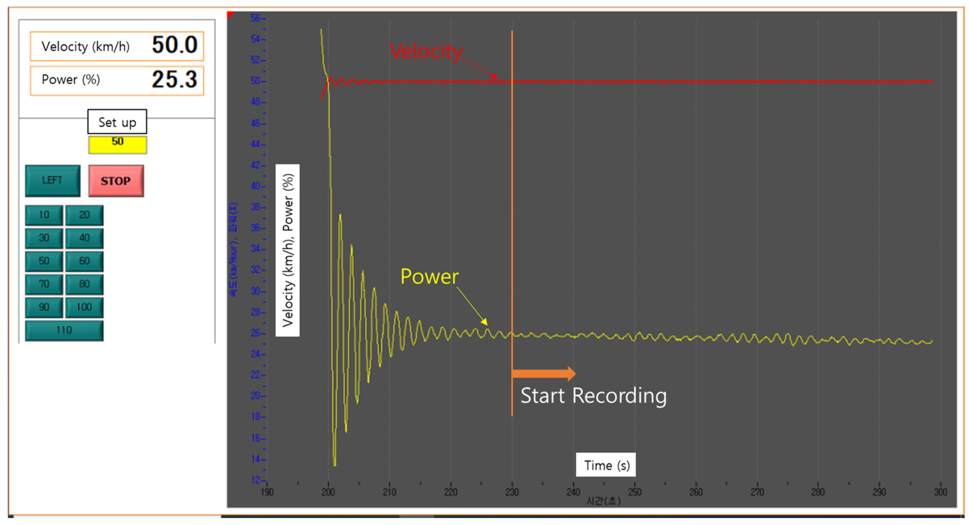
3.2. High-Speed Translational Moving Panel Device
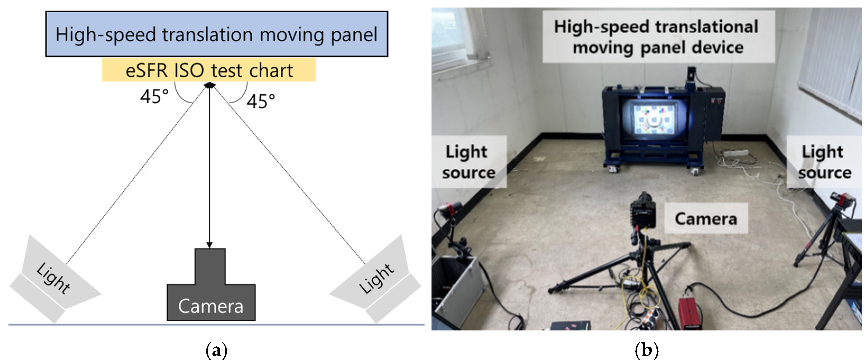
3.3. Indoor Test Setup in Standard Environments Considering Camera Exposure
4. Results
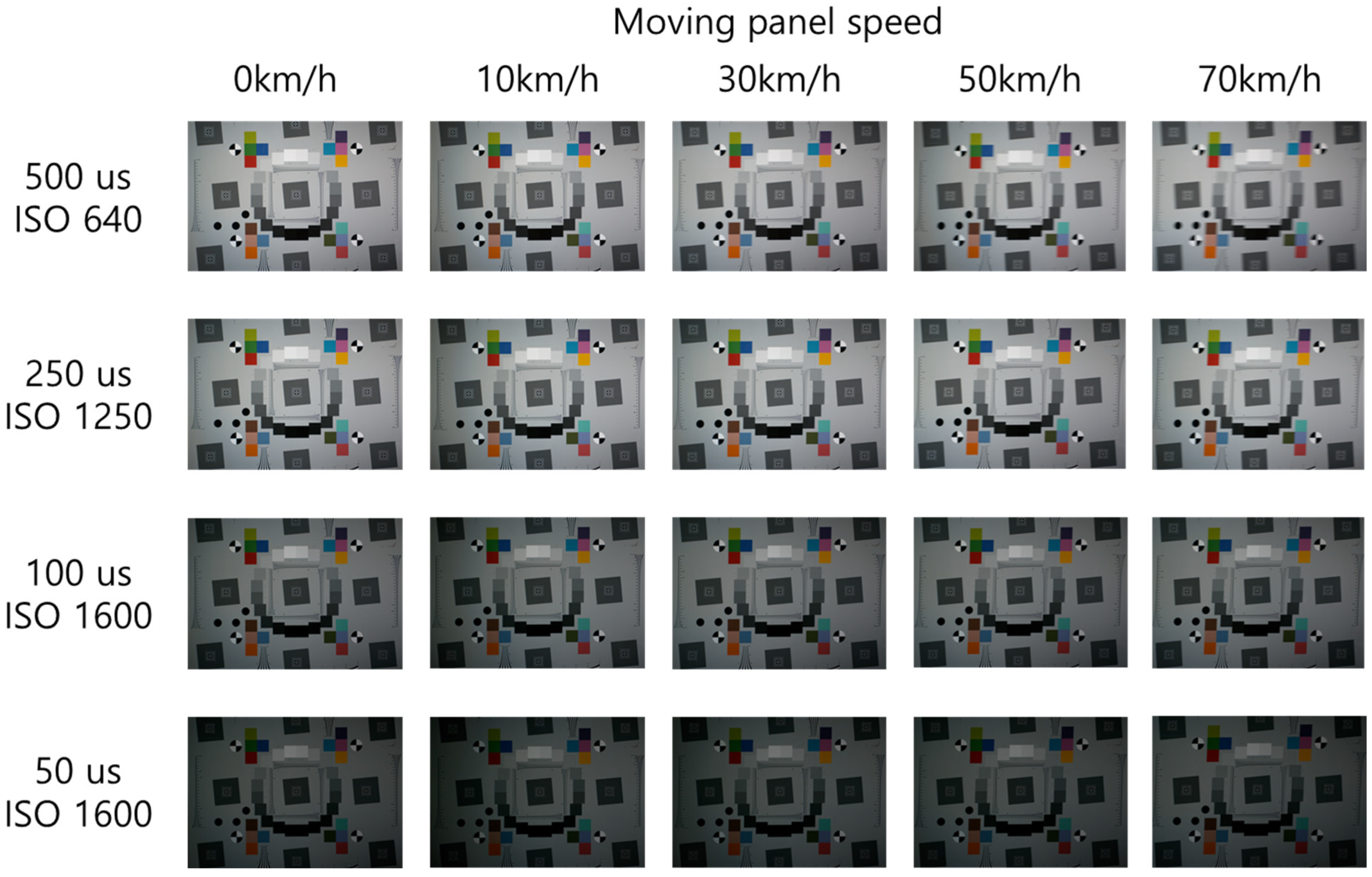
4.1. Analysis of BEW and MTF50 by Moving Speed and Shutter Speed
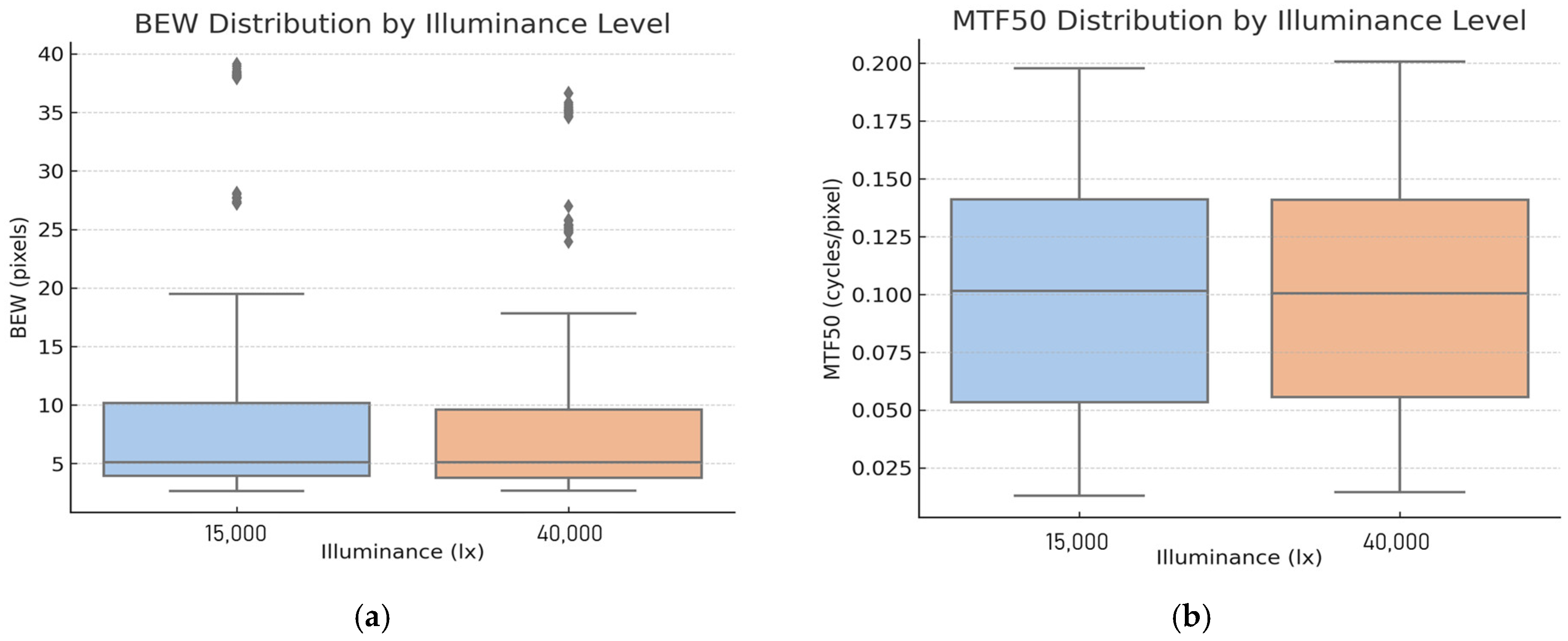
4.2. Analysis of Image Quality Variation Due to Increased Illuminance
4.3. Field Validation
5. Discussion
6. Conclusions
Author Contributions
Funding
Institutional Review Board Statement
Informed Consent Statement
Data Availability Statement
Acknowledgments
Conflicts of Interest
References
- Montero, R.; Victores, J.G.; Martínez, S.; Jardón, A.; Balaguer, C. Past, present and future of robotic tunnel inspection. Autom. Constr. 2015, 59, 99–112. [Google Scholar] [CrossRef]
- NTSB. Ceiling Collapse in the Interstate 90 Connector Tunnel; National Transportation Safety Board: Boston, MA, USA, 2006. [Google Scholar]
- Kawahara, S.; Doi, H.; Shirato, M.; Kajifusa, N.; Kutsukake, T. Investigation of the tunnel ceiling collapse in the central expressway in Japan; TRB Paper Manuscript 14–2559. In Proceedings of the Transportation Research Board 93rd Annual Meeting, Washington, DC, USA, 12–16 January 2014. [Google Scholar]
- Allaix, D.L.; Vliet, A.B. Existing standardization on monitoring, safety assessment and maintenance of bridges and tunnels. Ce/Pap. 2023, 6, 498–504. [Google Scholar] [CrossRef]
- Huang, Z.; Zhang, C.L.; Fu, H.L.; Ma, S.K.; Fan, X.D. Machine inspection equipment for tunnels: A review. J. Highw. Transp. Res. Dev. 2021, 15, 40–53. [Google Scholar] [CrossRef]
- Balaguer, C.; Montero, R.; Victores, J.G.; Martínez, S.; Jardón, A. Towards fully automated tunnel inspection: A survey and future trends. In Proceedings of the 31st International Symposium on Automation and Robotics in Construction and Mining (ISARC), Sydney, Australia, 9–11 July 2014; pp. 19–33. [Google Scholar] [CrossRef]
- Spencer, B.F.; Hoskere, V.; Narazaki, Y. Advances in computer vision-based civil infrastructure inspection and monitoring. Engineering 2019, 5, 199–222. [Google Scholar] [CrossRef]
- Ye, X.W.; Jin, T.; Yun, C.B. A review on deep learning-based structural health monitoring of civil infrastructures. Smart Struct. Syst. 2019, 24, 567–585. [Google Scholar] [CrossRef]
- Guo, J.; Liu, P.; Xiao, B.; Deng, L.; Wang, Q. Surface defect detection of civil structures using images: Review from data perspective. Autom. Constr. 2024, 158, 105186. [Google Scholar] [CrossRef]
- Sony, S.; Dunphy, K.; Sadhu, A.; Capretz, M. A systematic review of convolutional neural network-based structural condition assessment techniques. Eng. Struct. 2021, 226, 111347. [Google Scholar] [CrossRef]
- Sankarasrinivasan, S.; Balasubramanian, E.; Karthik, K.; Chandrasekar, U.; Gupta, R. Health monitoring of civil structures with integrated UAV and image processing system. Procedia Comput. Sci. 2015, 54, 508–515. [Google Scholar] [CrossRef]
- Landstrom, A.; Thurley, M.J. Morphology-based crack detection for steel slabs. IEEE J. Sel. Top. Signal Process. 2012, 7, 866–875. [Google Scholar] [CrossRef]
- Giakoumis, I.; Nikolaidis, N.; Pitas, I. Digital image processing techniques for the detection and removal of cracks in digitized paintings. IEEE Trans. Image Process. 2006, 15, 178–188. [Google Scholar] [CrossRef]
- Ranjan, P.; Chandra, U. A novel technique for wall crack detection using image fusion. In Proceedings of the International Conference on Computing, Communication and Informatics, Coimbatore, India, 4–6 January 2013; pp. 1–6. [Google Scholar]
- Cornelis, M.; Coscarón, M.C. The Nabidae (Insecta, Hemiptera, Heteroptera) of Argentina. Zookeys 2013, 333, 1–30. [Google Scholar] [CrossRef] [PubMed]
- Surace, C.; Ruotolo, R. Crack detection of a beam using the wavelet transform. In Proceedings of the International Symposium on Optics, Imaging, and Instrumentation, San Diego, CA, USA, 24–25 July 1994; p. 1141. [Google Scholar]
- Yamaguchi, T.; Nakamura, S.; Saegusa, R.; Hashimoto, S. Image-based crack detection for real concrete surfaces. IEEJ Trans. Electr. Electron. Eng. 2008, 3, 128–135. [Google Scholar] [CrossRef]
- Adhikari, R.S.; Moselhi, O.; Bagchi, A. Image-based retrieval of concrete crack properties for bridge inspection. Autom. Constr. 2014, 39, 180–194. [Google Scholar] [CrossRef]
- Nguyen, H.N.; Kam, T.Y.; Cheng, P.Y. An automatic approach for accurate edge detection of concrete crack utilizing 2D geometric features of crack. J. Sign. Process. Syst. 2014, 77, 221–240. [Google Scholar] [CrossRef]
- Xiang, C.; Wang, W.; Deng, L.; Shi, P.; Kong, X. Crack detection algorithm for concrete structures based on super-resolution reconstruction and segmentation network. Autom. Constr. 2022, 140, 104346. [Google Scholar] [CrossRef]
- Yao, Y.; Tung, S.E.; Glisic, B. Crack detection and characterization techniques—An overview. Struct. Control Health Monit. 2014, 21, 1387–1413. [Google Scholar] [CrossRef]
- Alidoost, F.; Austen, G.; Hahn, M. A multi-camera mobile system for tunnel inspection. In iCity: Transformative Research for the Livable, Intelligent, and Sustainable City; Coors, V., Pietruschka, D., Zeitler, B., Eds.; Springer International Publishing: Cham, Switzerland, 2022; pp. 211–224. [Google Scholar] [CrossRef]
- Yu, Y.; Samali, B.; Rashidi, M.; Mohammadi, M.; Nguyen, T.N.; Zhang, G. Vision-based concrete crack detection using a hybrid framework considering noise effect. J. Build. Eng. 2022, 61, 105246. [Google Scholar] [CrossRef]
- Ni, F.; Zhang, J.; Noori, M.N. Deep learning for data anomaly detection and data compression of a long-span suspension bridge. Comput. Aided Civ. Infrastruct. Eng. 2020, 35, 685–700. [Google Scholar] [CrossRef]
- Ukai, M.; Miyamoto, T.; Sasama, H. Development of inspection system of railway facilities using continuous scan image. WIT Trans. Built Environ. 1996, 20, 61–70. [Google Scholar]
- Sasama, H.; Ukai, M.; Ohta, M.; Miyamoto, T. Inspection system for railway facilities using a continuously scanned image. Electr. Eng. Japan 1998, 125, 52–64. [Google Scholar] [CrossRef]
- Ukai, M. Advanced inspection system of tunnel wall deformation using image processing. Q. Rep. RTRI 2007, 48, 94–98. [Google Scholar] [CrossRef]
- Yu, S.N.; Jang, J.H.; Han, C.S. Auto inspection system using a mobile robot for detecting concrete cracks in a tunnel. Autom. Constr. 2007, 16, 255–261. [Google Scholar] [CrossRef]
- Lee, S.Y.; Lee, S.H.; Shin, D.I.; Son, Y.K.; Han, C.S. Development of an inspection system for cracks in a concrete tunnel lining. Can. J. Civ. Eng. 2007, 34, 966–975. [Google Scholar] [CrossRef]
- Zhang, W.; Zhang, Z.; Qi, D.; Liu, Y. Automatic crack detection and classification method for subway tunnel safety monitoring. Sensors 2014, 14, 19307–19328. [Google Scholar] [CrossRef]
- Huang, H.; Sun, Y.; Xue, Y.; Wang, F. Inspection equipment study for subway tunnel defects by grey-scale image processing. Adv. Eng. Inform. 2017, 32, 188–201. [Google Scholar] [CrossRef]
- Gong, Q.; Zhu, L.; Wang, Y.; Yu, Z. Automatic subway tunnel crack detection system based on line scan camera. Struct. Control. Health Monit. 2021, 28, e2776. [Google Scholar] [CrossRef]
- Qin, S.; Qi, T.; Lei, B.; Li, Z. Rapid and automatic image acquisition system for structural surface defects of high-speed rail tunnels. KSCE J. Civ. Eng. 2024, 28, 967–989. [Google Scholar] [CrossRef]
- Zhan, D.; Yu, L.; Xiao, J.; Chen, T. Multi-camera and structured-light vision system (MSVS) for dynamic high-accuracy 3D measurements of railway tunnels. Sensors 2015, 15, 8664–8684. [Google Scholar] [CrossRef]
- Xiao, L.; Ying-jie, D.; Chun-ming, X.; Bo, L.; Yang, L. Design and implement of vehicle-based experiment prototype for expressway tunnel intelligent detection. In Proceedings of the 3rd International Conference on Robotics, Control and Automation, Chengdu, China, 11–13 August 2018; pp. 78–81. [Google Scholar] [CrossRef]
- Jiang, Y.; Zhang, X.; Taniguchi, T. Quantitative condition inspection and assessment of tunnel lining. Autom. Constr. 2019, 102, 258–269. [Google Scholar] [CrossRef]
- Gavilán, M.; Sánchez, F.; Ramos, J.A.; Marcos, O. Mobile inspection system for high-resolution assessment of tunnels. In Proceedings of the 6th International Conference on Structural Health Monitoring of Intelligent Infrastructure, Hong Kong, China, 9–11 December 2013. [Google Scholar]
- Yasuda, T.; Yamamoto, H.; Shigeta, Y. Tunnel inspection system by using high-speed mobile 3D survey vehicle: MIMM-R. J. Robot. Soc. Japan 2016, 34, 589–590. [Google Scholar] [CrossRef]
- Yasuda, T.; Yamamoto, H.; Enomoto, M.; Nitta, Y. Smart tunnel inspection and assessment using mobile inspection vehicle, non-contact radar and AI. From demonstration to practical use to new stage of construction robot. In Proceedings of the 37th International Symposium on Automation and Robotics in Construction 2020 (ISARC 2020), Kitakyushu, Japan, 27–28 October 2020; pp. 1373–1379. [Google Scholar] [CrossRef]
- MMSD. Available online: https://www.mitsubishielectric.co.jp/mmsd/ (accessed on 10 March 2024).
- Tunnel Catcher 3. Available online: https://mestrc.co.jp/radar/ (accessed on 10 March 2024).
- Tunnel Tracer. Available online: https://www.chugai-tec.co.jp/business/structure_material_investigation/ (accessed on 10 March 2024).
- GT-8K. Available online: https://www.aeroasahi.co.jp/company/fortune/157/ (accessed on 10 March 2024).
- Wang, H.; Wang, Q.; Zhai, J.; Yuan, D.; Zhang, W.; Xie, X.; Zhou, B.; Cai, J.; Lei, Y. Design of fast acquisition system and analysis of geometric feature for highway tunnel lining cracks based on machine vision. Appl. Sci. 2022, 12, 2516. [Google Scholar] [CrossRef]
- Xue, Y.; Li, Y. A fast detection method via region-based fully convolutional neural networks for shield tunnel lining defects. Comput. Aided Civ. Infrast. Eng. 2018, 33, 638–654. [Google Scholar] [CrossRef]
- Szegedy, C.; Liu, W.; Jia, Y.; Sermanet, P.; Reed, S.; Anguelov, D.; Erhan, D.; Vanhoucke, V.; Rabinovich, A. Going deeper with convolutions. In Proceedings of the 2015 IEEE Conference on Computer Vision and Pattern Recognition, Boston, MA, USA, 7–12 June 2015; pp. 1–9. [Google Scholar] [CrossRef]
- Krizhevsky, A.; Sutskever, I.; Hinton, G.E. Imagenet classification with deep convolutional neural networks. In Proceedings of the 25th International Conference on Neural Information Processing Systems, Lake Tahoe, NV, USA, 3–6 December 2012; Volume 25, pp. 1097–1105. [Google Scholar]
- Kim, B.; Cho, S. Automated vision-based detection of cracks on concrete surfaces using a deep learning technique. Sensors 2018, 18, 3452. [Google Scholar] [CrossRef] [PubMed]
- Zeiler, M.D.; Fergus, R. Visualizing and understanding convolutional networks. In Proceedings of the 13th European Conference on Computer Vision, Zurich, Switzerland, 6–12 September 2014; Springer: Cham, Switzerland, 2014; pp. 818–833. [Google Scholar] [CrossRef]
- Simonyan, K.; Zisserman, A. Very deep convolutional networks for large-scale image recognition. arXiv 2014, arXiv:1409.1556. [Google Scholar]
- Huang, H.; Li, Q.; Zhang, D. Deep learning-based image recognition for crack and leakage defects of metro shield tunnel. Tunn. Undergr. Space Technol. 2018, 77, 166–176. [Google Scholar] [CrossRef]
- Kamdi, S.; Krishna, R.K. Image segmentation and region growing algorithm. Int. J. Comput. Technol. Electr. Eng. 2012, 2, 103–107. [Google Scholar]
- Chan, F.Y.; Lam, F.K.; Zhu, H. Adaptive thresholding by variational method. IEEE Trans. Image Process. 1998, 7, 468–473. [Google Scholar] [CrossRef]
- Song, Q.; Wu, Y.; Xin, X.; Yang, L.; Yang, M.; Chen, H.; Liu, C.; Hu, M.; Chai, X.; Li, J. Real-time tunnel crack analysis system via deep learning. IEEE Access 2019, 7, 64186–64197. [Google Scholar] [CrossRef]
- Li, D.; Xie, Q.; Gong, X.; Yu, Z.; Xu, J.; Sun, Y.; Wang, J. Automatic defect detection of metro tunnel surfaces using a vision-based inspection system. Adv. Eng. Inform. 2021, 47, 101206. [Google Scholar] [CrossRef]
- Bae, H.; Jang, K.; An, K. Deep super resolution crack network (SrcNet) for improving computer vision–based automated crack detectability in in situ bridges. Struct. Health Monit. 2021, 20, 1428–1442. [Google Scholar] [CrossRef]
- Liu, Y.; Yeoh, J.K.W.; Chua, D.K.H. Deep learning-based enhancement of motion blurred UAV concrete crack images. J. Comput. Civ. Eng. 2020, 34, 04020028. [Google Scholar] [CrossRef]
- Sorel, M.; Flusser, J. Space-variant restoration of images degraded by camera motion blur. IEEE Trans. Image Process. 2008, 17, 105–116. [Google Scholar] [CrossRef] [PubMed]
- Paramanand, C.; Rajagopalan, A.N. Shape from sharp and motion-blurred image pair. Int. J. Comput. Vis. 2014, 107, 272–292. [Google Scholar] [CrossRef]
- Abdullah-Al-Mamun, M.; Tyagi, V.; Zhao, H. A new full-reference image quality metric for motion blur profile characterization. IEEE Access 2021, 9, 156361–156371. [Google Scholar] [CrossRef]
- Galoogahi, H.K.; Fagg, A.; Huang, C.; Ramanan, D.; Lucey, S. Need for speed: A benchmark for higher frame rate object tracking. In Proceedings of the IEEE International Conference on Computer Vision, Venice, Italy, 22–29 October 2017; pp. 1134–1143. [Google Scholar] [CrossRef]
- Su, S.; Delbracio, M.; Wang, J.; Sapiro, G.; Heidrich, W.; Wang, O. Deep video deblurring for hand-held cameras. In Proceedings of the IEEE Conference on Computer Vision and Pattern Recognition, Honolulu, HI, USA, 21–26 July 2017; pp. 237–246. [Google Scholar] [CrossRef]
- Nah, S.; Kim, T.H.; Lee, K.M. Deep multi-scale convolutional neural network for dynamic scene deblurring. In Proceedings of the IEEE Conference on Computer Vision and Pattern Recognition, Honolulu, HI, USA, 21–26 July 2017; pp. 257–265. [Google Scholar] [CrossRef]
- Nah, S.; Baik, S.; Hong, S.; Moon, G.; Son, S.; Timofte, R.; Mu Lee, K. NTIRE 2019 challenge on video deblurring and super-resolution: Dataset and study. In Proceedings of the 2019 IEEE/CVF Conference on Computer Vision and Pattern Recognition Workshops (CVPRW), Long Beach, CA, USA, 16–17 June 2019; pp. 1996–2005. [Google Scholar] [CrossRef]
- Shen, Z.; Wang, W.; Lu, X.; Shen, J.; Ling, H.; Xu, T.; Shao, L. Human-aware motion deblurring. In Proceedings of the IEEE/CVF International Conference on Computer Vision (ICCV), Seoul, Republic of Korea, 27 October–2 November 2019; pp. 5571–5580. [Google Scholar] [CrossRef]
- Rim, J.; Lee, H.; Won, J.; Cho, S. Real-world blur dataset for learning and benchmarking deblurring algorithms. In Computer Vision—ECCV 2020; Vedaldi, A., Bischof, H., Brox, T., Frahm, J.M., Eds.; Springer International Publishing: Cham, Switzerland, 2020; pp. 184–201. [Google Scholar] [CrossRef]
- Jiang, H.; Sun, D.; Jampani, V.; Yang, M.H.; Learned-Miller, E.; Kautz, J. Super SloMo: High quality estimation of multiple intermediate frames for video interpolation. In Proceedings of the IEEE Conference on Computer Vision and Pattern Recognition, Salt Lake City, UT, USA, 18–22 June 2018; pp. 9000–9008. [Google Scholar] [CrossRef]
- De, K.D.; Masilamani, V. Image sharpness measure for blurred images in frequency domain. Procedia Eng. 2013, 64, 149–158. [Google Scholar] [CrossRef]
- Wang, Z.; Bovik, A.C.; Sheikh, H.R.; Simoncelli, E.P. Image quality assessment: From error visibility to structural similarity. IEEE Trans. Image Process. 2004, 13, 600–612. [Google Scholar] [CrossRef]
- Moorthy, A.K.; Bovik, A.C. Blind image quality assessment: From natural scene statistics to perceptual quality. IEEE Trans. Image Process. 2011, 20, 3350–3364. [Google Scholar] [CrossRef]
- Salomon, D.; Motta, G. Handbook of Data Compression; Springer: New York, NY, USA, 2010. [Google Scholar] [CrossRef]
- Horé, A.; Ziou, D. Image quality metrics: PSNR vs. SSIM. In Proceedings of the 2010 20th International Conference on Pattern Recognition, Istanbul, Turkey, 23–26 August 2010; pp. 2366–2369. [Google Scholar] [CrossRef]
- Kamble, V.; Bhurchandi, K.M. No-reference image quality assessment algorithms: A survey. Optik 2015, 126, 1090–1097. [Google Scholar] [CrossRef]
- Dost, S.; Saud, F.; Shabbir, M.; Khan, M.G.; Shahid, M.; Lovstrom, B. Reduced reference image and video quality assessments: Review of methods. EURASIP J. Image Video Process. 2022, 2022, 1. [Google Scholar] [CrossRef]
- Sheikh, H. Live Image Quality Assessment Database Release 2. Available online: http://live.ece.utexas.edu/research/quality (accessed on 10 March 2024).
- Ponomarenko, N.; Lukin, V.; Zelensky, A.; Egiazarian, K.; Carli, M.; Battisti, F. TID2008-a database for evaluation of full-reference visual quality assessment metrics. Adv. Mod. Radioelectron. 2009, 10, 30–45. [Google Scholar]
- Ponomarenko, N.; Jin, L.; Ieremeiev, O.; Lukin, V.; Egiazarian, K.; Astola, J.; Vozel, B.; Chehdi, K.; Carli, M.; Battisti, F.; et al. Image database TID2013: Peculiarities, results and perspectives. Signal Process. Image Commun. 2015, 30, 57–77. [Google Scholar] [CrossRef]
- Corchs, S.; Gasparini, F.; Schettini, R. No reference image quality classification for JPEG-distorted images. Digit. Signal Process. 2014, 30, 86–100. [Google Scholar] [CrossRef]
- Imatest. Available online: https://www.imatest.com/ (accessed on 10 March 2024).
- Choi, S.; Jun, H.; Shin, S.; Chung, W. Evaluating accuracy of algorithms providing subsurface properties using full-reference image quality assessment. Geophys. Geophys. Explor. 2021, 24, 6–19. [Google Scholar]
- Dey, R.; Bhattacharjee, D.; Kejcar, O. No-reference image quality assessment using meta-learning. In COMSYS 2023, Volume 2, Proceedings of the International Conference on Frontiers of Computer Science and Technology, Himachal Pradesh, India, 16–17 October 2023; Sarkar, R., Pal, S., Basu, S., Plewczynski, D., Bhattacharjee, D., Eds.; Springer Nature: Singapore, 2023; pp. 137–144. [Google Scholar] [CrossRef]
- Bae, S.H.; Kim, M. Elaborate image quality assessment with a novel luminance adaptation effect model. J. Broadcast. Eng. 2015, 20, 818–826. [Google Scholar] [CrossRef]
- Dinh, H.; Wang, Q.; Tu, F.; Frymire, B.; Mu, B. Evaluation of motion blur image quality in video frame interpolation. Electron. Imaging 2023, 35, 262–265. [Google Scholar] [CrossRef]
- ISO 12233:2023; Photography: Electronic Still Picture Imaging—Resolution and Spatial Frequency Responses. International Organization for Standardization: Geneva, Switzerland, 2023. Available online: https://www.iso.org/obp/ui/#iso:std:iso:12233:ed-4:v1:en (accessed on 10 March 2024).
- Imatest—ISO 122233:2017 Test Charts. Available online: http://www.imatest.com/solutions/iso-12233/ (accessed on 10 March 2024).
- Masaoka, K. Accuracy and precision of edge-based modulation transfer function measurement for sampled imaging systems. IEEE Access 2018, 6, 41079–41086. [Google Scholar] [CrossRef]
- Imatest-Sharpness. 2023. Available online: https://www.imatest.com/support/docs/23-1/sharpness/ (accessed on 10 March 2024).
- Dugonik, B.; Dugonik, A.; Marovt, M.; Golob, M. Image quality assessment of digital image capturing devices for melanoma detection. Appl. Sci. 2020, 10, 2876. [Google Scholar] [CrossRef]
- Artmann, U. Image quality evaluation using moving targets. In Multimedia Content Mobile Devices; SPIE: Bellingham, WA, USA, 2013; Volume 8667, pp. 398–409. [Google Scholar] [CrossRef]
- Koren, N. The Imatest program: Comparing cameras with different amounts of sharpening. In Digital Photography II; SPIE: Bellingham, WA, USA, 2013; Volume 6069, pp. 195–203. [Google Scholar] [CrossRef]
- Imatest—MTF Curves and Image Appearance. Available online: https://www.imatest.com/docs/MTF_appearance/ (accessed on 10 March 2024).
- Luo, L.; Yurdakul, C.; Feng, K.; Seo, D.E.; Tu, F.; Mu, B. Temporal MTF evaluation of slow-motion mode in mobile phones. J. Electron. Imaging 2022, 34, 1–4. [Google Scholar] [CrossRef]
- Telleen, J.; Sullivan, A.; Yee, J.; Wang, O.; Gunawardane, P.; Collins, I.; Davis, J. Synthetic shutter speed imaging. Comput. Graph. Forum 2007, 26, 591–598. [Google Scholar] [CrossRef]
- Lee, G.P.; Lim, H.J.; Kim, J.H. Availability evaluation of automatic inspection equipment using line scan camera for concrete lining. J. Korean Tunn. Undergr. Space Assoc. 2020, 22, 643–653. [Google Scholar]
- Imatest-SFRreg Test Chart. 2024. Available online: https://www.imatest.com/product/sfrreg-test-chart/ (accessed on 10 March 2024).
- Narvekar, N.D.; Karam, L.J. A no-reference image blur metric based on the cumulative probability of blur detection (CPBD). IEEE Trans. Image Process. 2011, 20, 2678–2683. [Google Scholar] [CrossRef] [PubMed]
- Mittal, A.; Moorthy, A.K.; Bovik, A.C. No-reference image quality assessment in the spatial domain. IEEE Trans. Image Process. 2012, 21, 4695–4708. [Google Scholar] [CrossRef] [PubMed]
- Mittal, A.; Soundararajan, R.; Bovik, A.C. Making a completely blind image quality analyzer. IEEE Signal Process. Lett. 2012, 20, 209–212. [Google Scholar] [CrossRef]
- Venkatanath, N.; Praneeth, D.; Bh, M.C.; Channappayya, S.S.; Medasani, S.S. Blind image quality evaluation using perception based features. In Proceedings of the 2015 Twenty First National Conference on Communications (NCC), Mumbai, India, 27 February–1 March 2015; pp. 1–6. [Google Scholar] [CrossRef]
- Pennada, S.; Perry, M.; McAlorum, J.; Dow, H.; Dobie, G. Threshold-Based BRISQUE-Assisted Deep Learning for Enhancing Crack Detection in Concrete Structures. J. Imaging 2023, 9, 218. [Google Scholar] [CrossRef]


| Panel Speed (km/h) | Shutter Speed (μs) | ISO | F-Number | FPS | Illuminance |
|---|---|---|---|---|---|
| 0 10 30 50 70 | 500 | 640 | 2.8 | 100 | 15,000 lx 40,000 lx |
| 250 | 1250 | ||||
| 100 | 1600 | ||||
| 50 | 1600 |
| Shutter Speed | IQA | 0 km/h | 10 km/h | 30 km/h | 50 km/h | 70 km/h |
|---|---|---|---|---|---|---|
| 500 μs | BEW_mean (pixels) | 3.40 | 6.31 | 16.38 | 27.56 | 38.28 |
| BEW_std (pixels) | ±0.38 | ±0.25 | ±0.09 | ±0.28 | ±0.31 | |
| MTF50_mean (cy/px) | 0.1566 | 0.0810 | 0.0375 | 0.0271 | 0.0227 | |
| MTF50_std (cy/px) | ±0.0155 | ±0.0208 | ±0.0324 | ±0.0352 | ±0.0364 | |
| 250 μs | BEW_mean (pixels) | 3.61 | 4.68 | 8.78 | 13.86 | 18.99 |
| BEW_std (pixels) | ±0.41 | ±0.46 | ±0.12 | ±0.11 | ±0.29 | |
| MTF50_mean (cy/px) | 0.1485 | 0.1118 | 0.0606 | 0.0423 | 0.0338 | |
| MTF50_std (cy/px) | ±0.0133 | ±0.0154 | ±0.0262 | ±0.0311 | ±0.0334 | |
| 100 μs | BEW_mean (pixels) | 3.56 | 3.86 | 4.73 | 6.33 | 8.47 |
| BEW_std (pixels) | ±0.33 | ±0.74 | ±0.33 | ±0.21 | ±0.21 | |
| MTF50_mean (cy/px) | 0.1505 | 0.1445 | 0.1069 | 0.0806 | 0.0626 | |
| MTF50_std (cy/px) | ±0.0114 | ±0.0253 | ±0.0153 | ±0.0209 | ±0.0257 | |
| 50 μs | BEW_mean (pixels) | 3.37 | 3.66 | 3.99 | 4.52 | 5.32 |
| BEW_std (pixels) | ±0.26 | ±0.70 | ±0.5 | ±0.34 | ±0.43 | |
| MTF50_mean (cy/px) | 0.1581 | 0.1524 | 0.1337 | 0.1140 | 0.0955 | |
| MTF50_std (cy/px) | ±0.0128 | ±0.0253 | ±0.0162 | ±0.0143 | ±0.0182 |
| Shutter Speed | IQA | 0 km/h | 10 km/h | 30 km/h | 50 km/h | 70 km/h |
|---|---|---|---|---|---|---|
| 500 μs | BEW_mean (px) | 3.23 | 6.07 | 15.18 | 25.19 | 35.37 |
| BEW_std (px) | ±0.54 | ±0.34 | ±0.12 | ±0.51 | ±0.61 | |
| MTF50_mean (cy/px) | 0.1692 | 0.0853 | 0.0403 | 0.0295 | 0.0155 | |
| MTF50_std (cy/px) | ±0.0293 | ±0.0199 | ±0.0317 | ±0.0346 | ±0.0005 | |
| 250 μs | BEW_mean (px) | 3.52 | 4.39 | 8.29 | 12.83 | 17.44 |
| BEW_std (x) | ±0.47 | ±0.35 | ±0.12 | ±0.18 | ±0.2 | |
| MTF50_mean (cy/px) | 0.1634 | 0.1172 | 0.0583 | 0.0374 | 0.0277 | |
| MTF50_std (cy/px) | ±0.0166 | ±0.0068 | ±0.0014 | ±0.0008 | ±0.0006 | |
| 100 μs | BEW_mean (px) | 3.49 | 3.61 | 4.76 | 6.47 | 8.37 |
| BEW_std (px) | ±0.28 | ±0.31 | ±0.19 | ±0.15 | ±0.12 | |
| MTF50_mean (cy/px) | 0.1594 | 0.1456 | 0.1041 | 0.0743 | 0.0567 | |
| MTF50_std (cy/px) | ±0.0092 | ±0.0070 | ±0.0038 | ±0.0014 | ±0.0007 | |
| 50 μs | BEW_mean (px) | 3.42 | 3.71 | 3.95 | 4.43 | 5.30 |
| BEW_std (px) | ±0.16 | ±0.35 | ±0.24 | ±0.15 | ±0.18 | |
| MTF50_mean (cy/px) | 0.1569 | 0.1432 | 0.1337 | 0.1135 | 0.0897 | |
| MTF50_std (cy/px) | ±0.0063 | ±0.0098 | ±0.0056 | ±0.0029 | ±0.0022 |
| Illuminance | Metric |
Source of Variation | DF | Sum of Squares | F-Value | p-Value |
|---|---|---|---|---|---|---|
| 15,000 lx | BEW | Moving panel speed | 4 | 17,036.88 | 29,998.22 | <0.0001 |
| Shutter speed | 3 | 18,673.68 | 43,840.35 | <0.0001 | ||
| Interaction | 12 | 14,139.28 | 8298.73 | <0.0001 | ||
| Residual | 580 | 82.35 | - | <0.0001 | ||
| MTF50 | Moving panel speed | 4 | 0.82 | 365.26 | <0.0001 | |
| Shutter speed | 3 | 0.39 | 233.39 | <0.0001 | ||
| Interaction | 12 | 0.11 | 16.48 | <0.0001 | ||
| Residual | 580 | 0.32 | - | <0.0001 | ||
| 40,000 lx | BEW | Moving panel speed | 4 | 14,555.51 | 36,821.60 | <0.0001 |
| Shutter speed | 3 | 15,158.78 | 51,130.25 | <0.0001 | ||
| Interaction | 12 | 11,647.52 | 9821.72 | <0.0001 | ||
| Residual | 580 | 57.32 | - | <0.0001 | ||
| MTF50 | Moving panel speed | 4 | 1.04 | 1265.27 | <0.0001 | |
| Shutter speed | 3 | 0.32 | 523.77 | <0.0001 | ||
| Interaction | 12 | 0.15 | 59.73 | <0.0001 | ||
| Residual | 580 | 0.12 | - | <0.0001 |
| Moving Panel Speed (km/h) | Shutter Speed (μs) | BEW p-Value | MTF50 p-Value |
|---|---|---|---|
| 0 | 50 | 0.3372 | 0.644 |
| 100 | 0.3564 | 0.0014 (p < 0.05) | |
| 250 | 0.4386 | 0.0003 (p < 0.05) | |
| 500 | 0.1645 | 0.0435 (p < 0.05) | |
| 10 | 50 | 0.7409 | 0.0715 |
| 100 | 0.0944 | 0.8215 | |
| 250 | 0.0072 (p < 0.05) | 0.0903 | |
| 500 | 0.003 (p < 0.05) | 0.4239 | |
| 30 | 50 | 0.7071 | 0.9949 |
| 100 | 0.7594 | 0.3376 | |
| 250 | 0 (p < 0.05) | 0.6427 | |
| 500 | 0 (p < 0.05) | 0.733 | |
| 50 | 50 | 0.1816 | 0.8499 |
| 100 | 0.0029(p < 0.05) | 0.1083 | |
| 250 | 0 (p < 0.05) | 0.394 | |
| 500 | 0 (p < 0.05) | 0.7915 | |
| 70 | 50 | 0.7335 | 0.0965 |
| 100 | 0.019 (p < 0.05) | 0.214 | |
| 250 | 0 (p < 0.05) | 0.3242 | |
| 500 | 0 (p < 0.05) | 0.2914 |
| Metric | Illuminance | Q1 (25%) | Median (50%) | Q3 (75%) | Mean | Min | Max | Std. Dev. | Sample |
|---|---|---|---|---|---|---|---|---|---|
| BEW (pixels) | 15,000 lx | 3.94 | 5.13 | 10.17 | 9.48 | 2.65 | 39.14 | 9.13 | 600 |
| 40,000 lx | 3.79 | 5.1 | 9.59 | 8.95 | 2.67 | 36.64 | 8.32 | 600 | |
| MTF50 (cy/px) | 15,000 lx | 0.0534 | 0.1016 | 0.1411 | 0.096 | 0.013 | 0.1979 | 0.0524 | 600 |
| 40,000 lx | 0.0556 | 0.1005 | 0.141 | 0.0961 | 0.0145 | 0.2008 | 0.0521 | 600 |
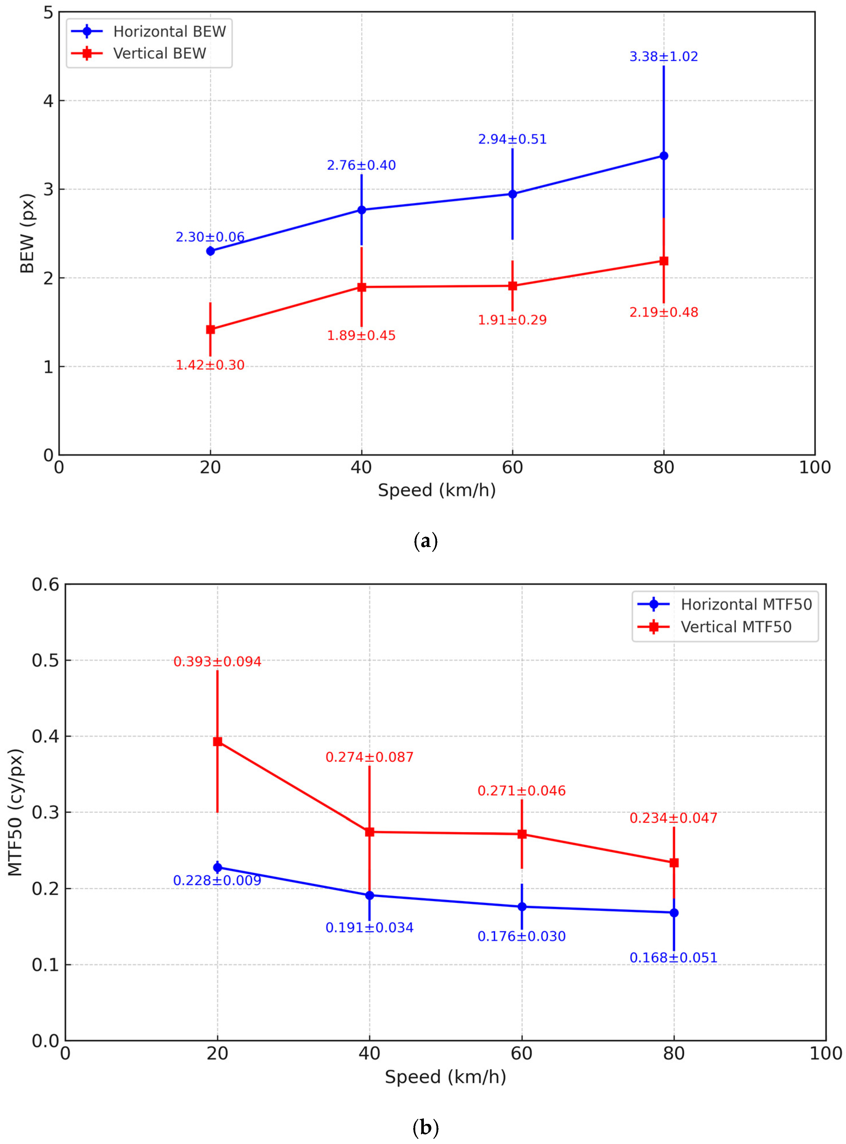
| Direction | Speed (km/h) | Mean BEW (px) | Std. Dev. | Mean MTF50 (cy/px) | Std. Dev. |
|---|---|---|---|---|---|
| Horizontal | 20 | 2.30 | ±0.06 | 0.228 | ±0.009 |
| 40 | 2.76 | ±0.40 | 0.191 | ±0.034 | |
| 60 | 2.94 | ±0.51 | 0.176 | ±0.030 | |
| 80 | 3.38 | ±1.02 | 0.168 | ±0.051 | |
| Vertical | 20 | 1.42 | ±0.30 | 0.393 | ±0.094 |
| 40 | 1.89 | ±0.45 | 0.274 | ±0.087 | |
| 60 | 1.91 | ±0.29 | 0.271 | ±0.046 | |
| 80 | 2.19 | ±0.48 | 0.234 | ±0.047 |
Disclaimer/Publisher’s Note: The statements, opinions and data contained in all publications are solely those of the individual author(s) and contributor(s) and not of MDPI and/or the editor(s). MDPI and/or the editor(s) disclaim responsibility for any injury to people or property resulting from any ideas, methods, instructions or products referred to in the content. |
© 2025 by the authors. Licensee MDPI, Basel, Switzerland. This article is an open access article distributed under the terms and conditions of the Creative Commons Attribution (CC BY) license (https://creativecommons.org/licenses/by/4.0/).
Share and Cite
Lee, C.; Kim, D.; Kim, D. Quality Assessment of High-Speed Motion Blur Images for Mobile Automated Tunnel Inspection. Sensors 2025, 25, 3804. https://doi.org/10.3390/s25123804
Lee C, Kim D, Kim D. Quality Assessment of High-Speed Motion Blur Images for Mobile Automated Tunnel Inspection. Sensors. 2025; 25(12):3804. https://doi.org/10.3390/s25123804
Chicago/Turabian StyleLee, Chulhee, Donggyou Kim, and Dongku Kim. 2025. "Quality Assessment of High-Speed Motion Blur Images for Mobile Automated Tunnel Inspection" Sensors 25, no. 12: 3804. https://doi.org/10.3390/s25123804
APA StyleLee, C., Kim, D., & Kim, D. (2025). Quality Assessment of High-Speed Motion Blur Images for Mobile Automated Tunnel Inspection. Sensors, 25(12), 3804. https://doi.org/10.3390/s25123804