

A Dynamic Self-Adjusting System for Permanent Magnet Synchronous Motors Using an Improved Super-Twisting Sliding Mode Observer


Abstract
1. Introduction
- An improved error function replaces the piecewise function, enabling automatic adjustment of the system through the adjustment of the error factor without considering the selection of the boundary layer, significantly reducing the workload.
- A comprehensive analysis of the impact of the error factor in SMOs is conducted, including observations of estimated current, speed, and position, summarizing corresponding patterns. Specifically, the chattering in SMOs decreases and then increases with the increase in the error factor, while the estimation error also decreases and then increases with the error factor. As the SMO state moves away from the sliding mode surface, the accuracy of the estimated position declines, ultimately reducing control precision. Based on this pattern, selection criteria for the error factor are derived, emphasizing the need to balance chattering suppression and control precision maintenance.
- Combining the patterns and selection criteria from the error factor impact analysis, a neural-network-error-factor self-adjusting SMO model is designed. This method not only considers the balance between chattering and control precision but also significantly reduces design workload, allowing for self-adjustment of the error factor based on actual working conditions. Finally, simulations and experimental validations in the MATLAB/Simulink environment demonstrate that the proposed method exhibits good feasibility and effectiveness, providing new ideas and methods for sensorless control technologies in PMSMs. This research not only enriches the theoretical framework of sliding mode observers but also offers strong support for practical engineering applications.
2. Traditional Sliding Mode Observation Method
2.1. Traditional Sliding Mode Observer
2.2. Sliding Mode Observer
2.3. Stability Analysis
3. Selection of the Error Factor
3.1. Impact Analysis of the Error Factor
3.2. Establishing the Error Factor Using Neural Network Algorithms
4. Simulation Verification
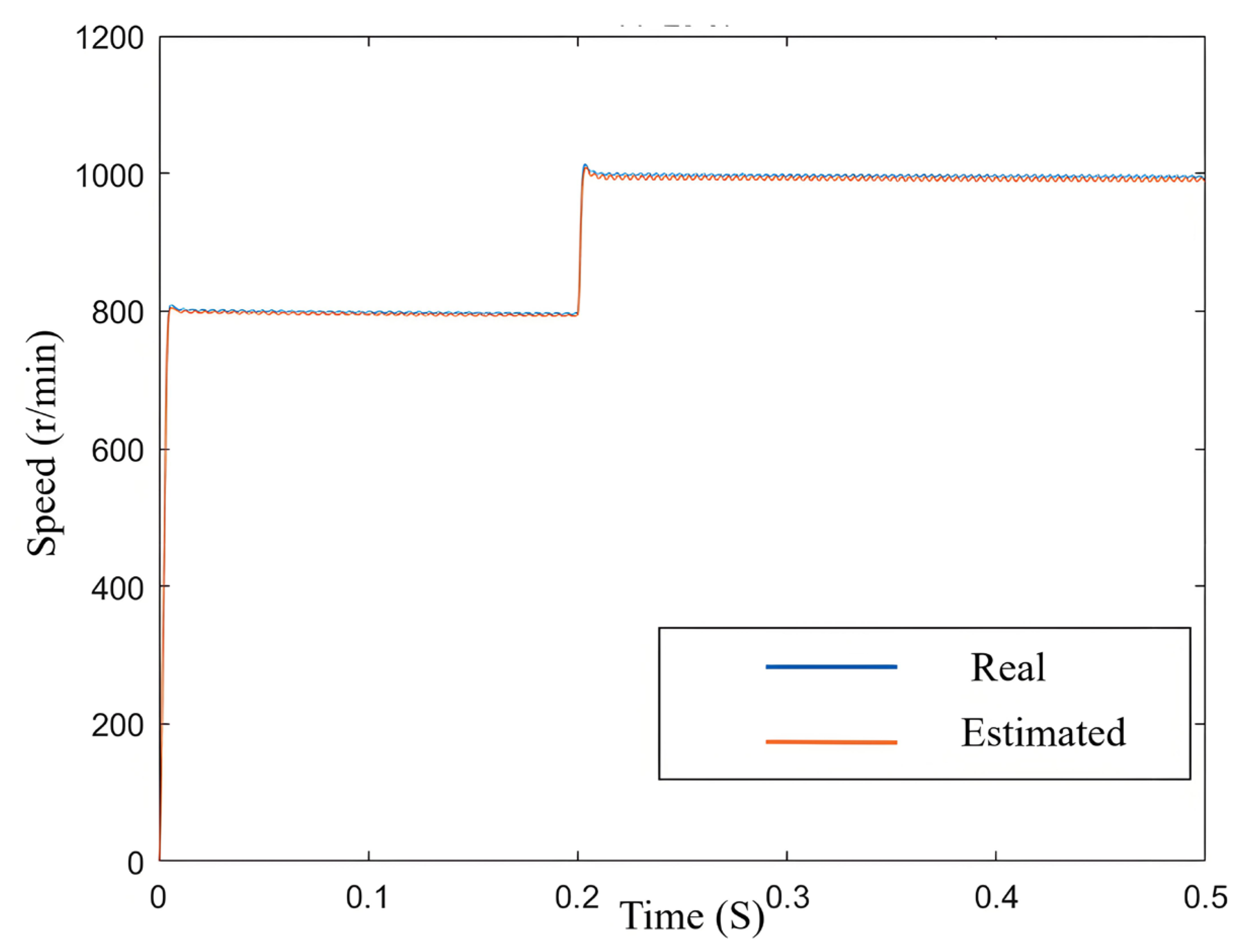
4.1. Speed Variation Analysis
4.2. Sudden Increase Load Analysis
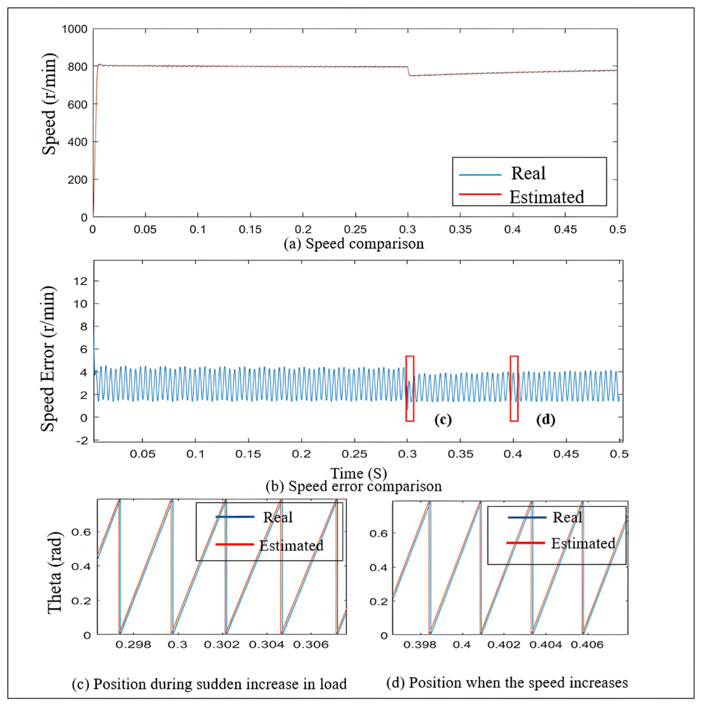
4.2.1. Simulation Verification Under Sudden Load
4.2.2. Effectiveness Verification During Sudden Load Increase
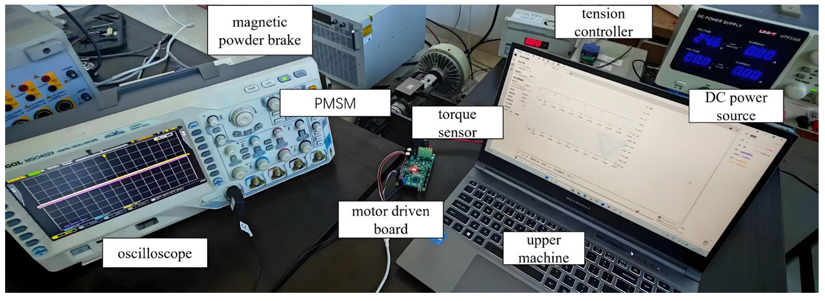
5. Experimental Verification
5.1. Verification of Speed Variation for Self-Adjusting Error Factor SMO
5.1.1. Comparison of Speed Increase and Decrease Experiments
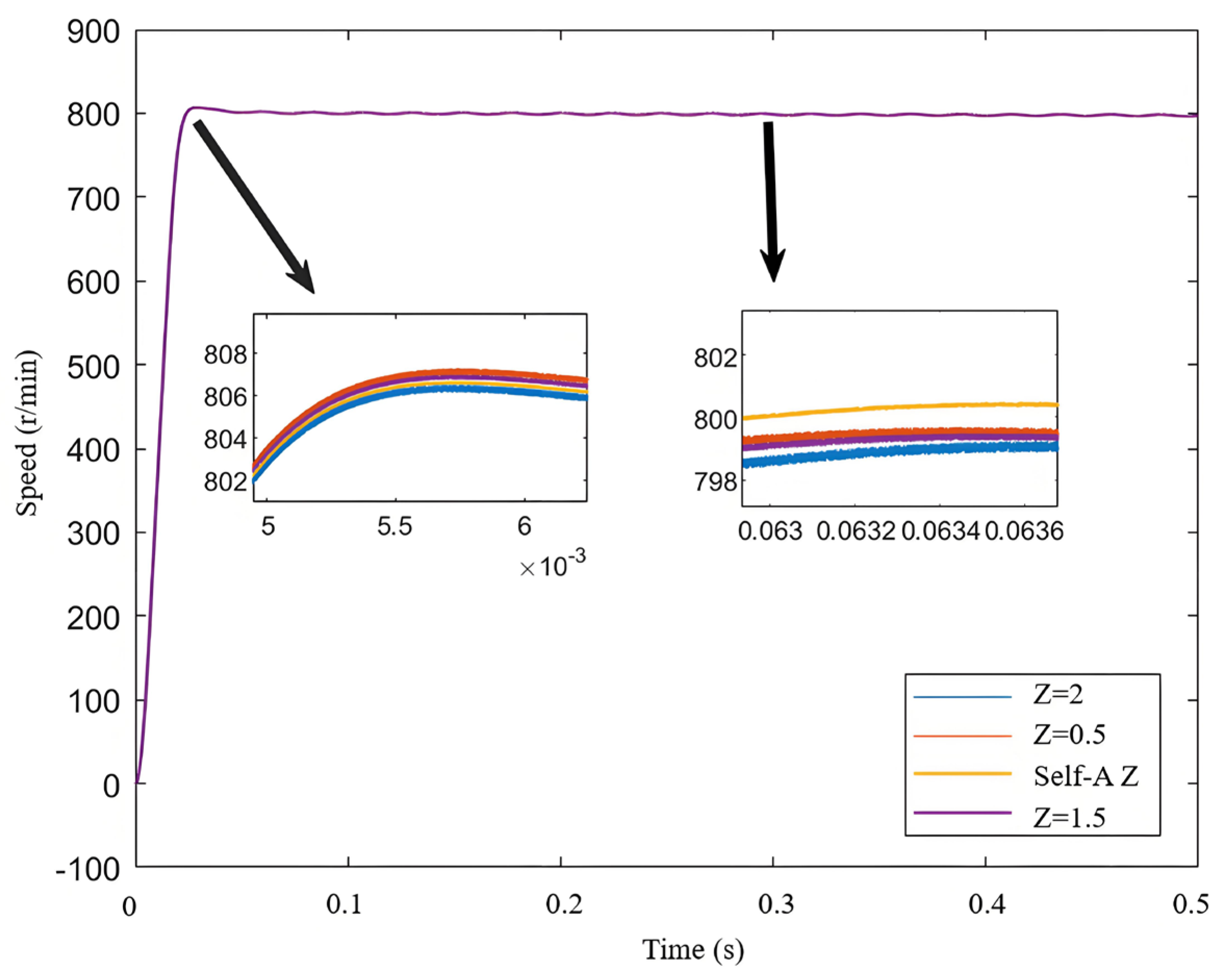
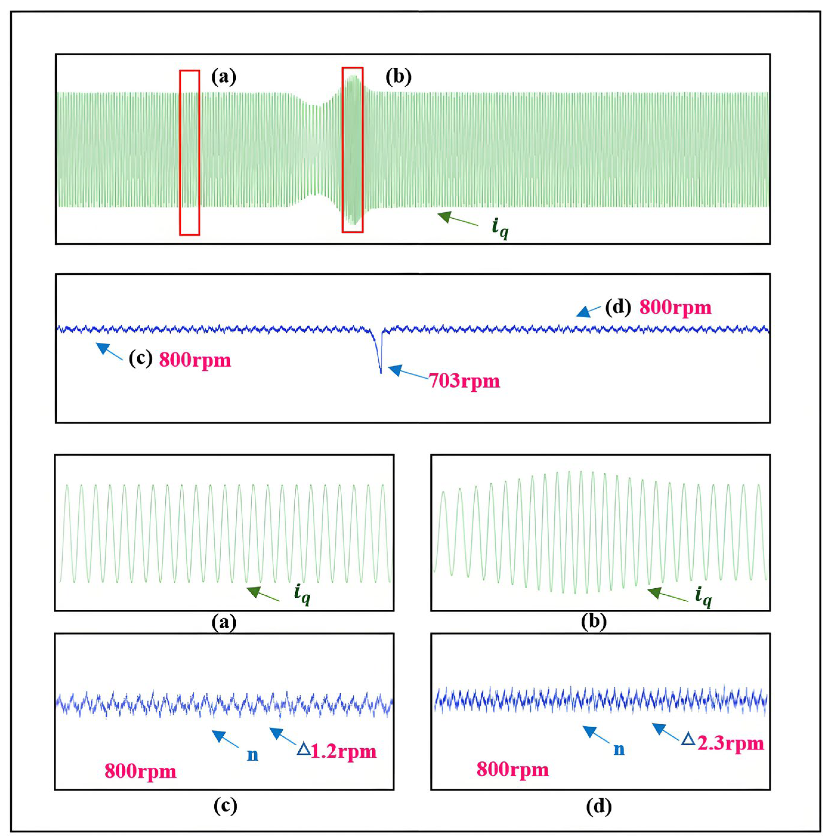
5.1.2. Verification of Effectiveness of Self-Adjusting Z Value During Speed Increase
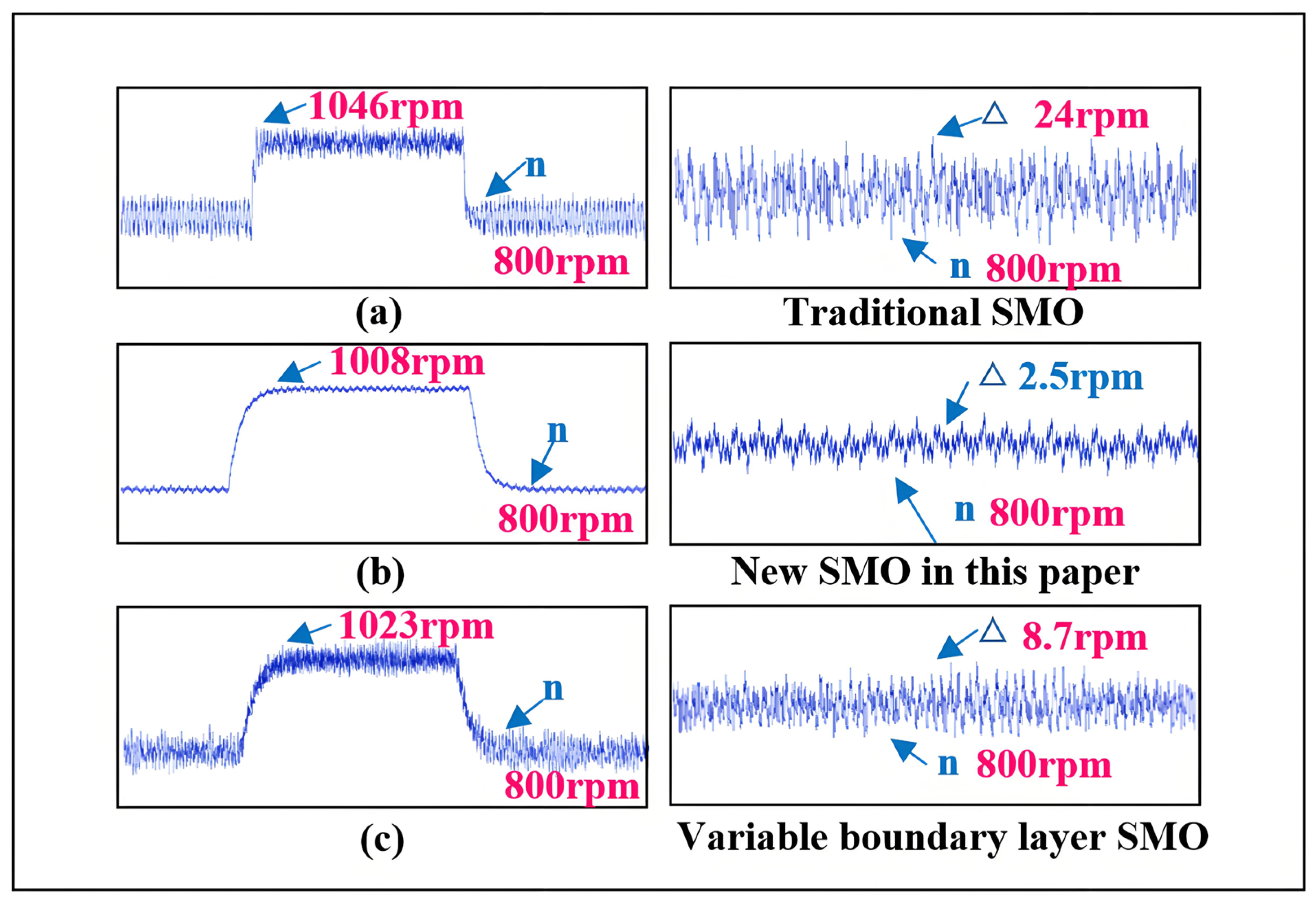
5.1.3. Verification of Effectiveness of the Novel SMO During Speed Increase and Decrease
5.2. Verification of Self-Adjusting Error Factor SMO Under Sudden Load Increase
5.2.1. Feasibility Verification During Sudden Load Increase
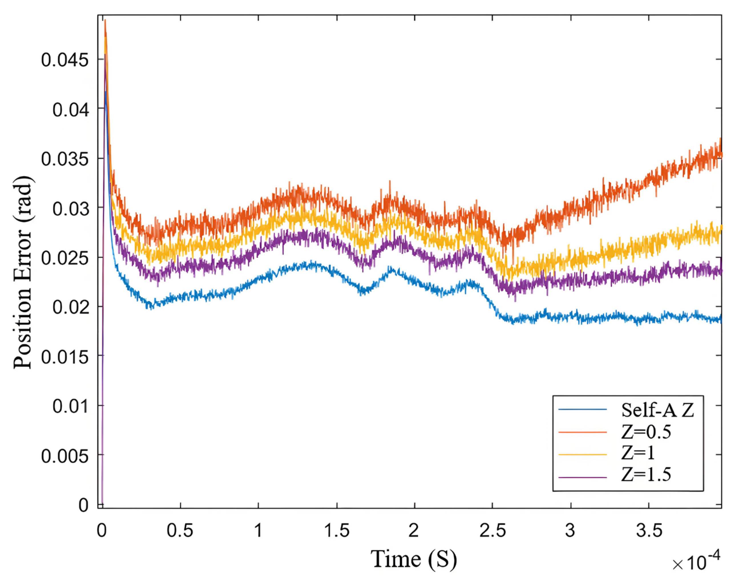
5.2.2. Effectiveness Verification of Self-Adjusting Z Value During Sudden Load Increase
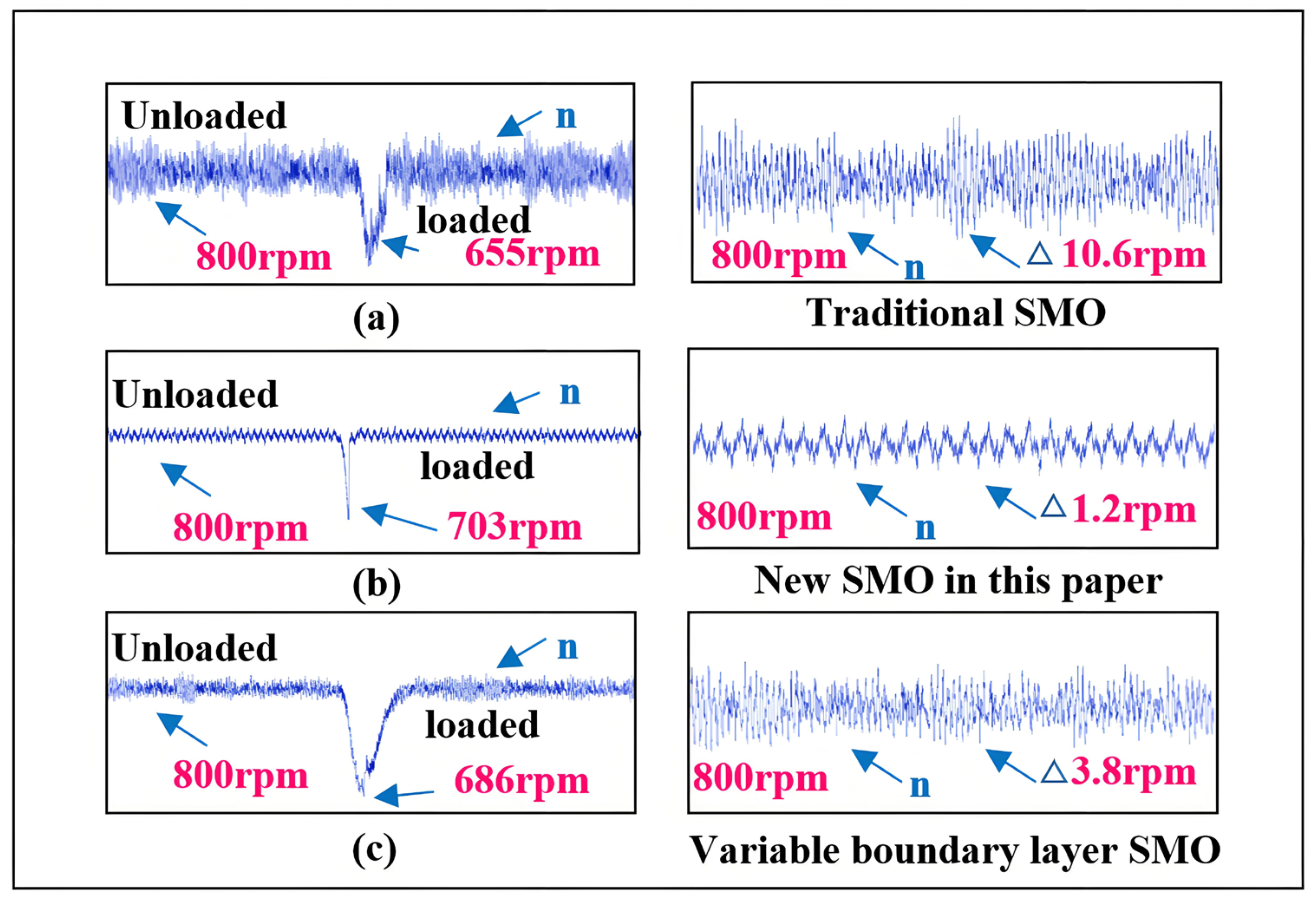
5.2.3. Effectiveness Verification of the Novel SMO During Sudden Load Increase
5.3. Comparative Experimental Analysis
5.3.1. Quantitative Influence Experiment of Parameter Perturbation on System Efficiency
- (1)
- The dynamic gain regulation of the neural network suppresses the current harmonics and reduces the THD by 40–50%.
- (2)
- The adaptive observer reduces the switching loss of the inverter by 25~30%.
5.3.2. Performance Analysis
6. Conclusions
Author Contributions
Funding
Institutional Review Board Statement
Informed Consent Statement
Data Availability Statement
Conflicts of Interest
References
- Guo, B.; Su, M.; Wang, H.; Tang, Z.; Liao, Y.; Zhang, L.; Shi, S. Observer-based second-order sliding mode control for grid-connected VSI with LCL-type filter under weak grid. Electr. Power Syst. Res. 2020, 183, 106270. [Google Scholar] [CrossRef]
- Vural, B.; Dusmez, S.; Uzunoglu, M.; Ugur, E.; Akin, B. Fuel consumption comparison of different battery/ultracapacitor hybridization topologies for fuel-cell vehicles on a test bench. IEEE J. Emerg. Sel. Top. Power Electron. 2014, 2, 552–561. [Google Scholar] [CrossRef]
- Li, L.; Liao, S.; Zou, B.; Liu, J. Mechanism-Based Fault Diagnosis Deep Learning Method for Permanent Magnet Synchronous Motor. Sensors 2024, 24, 6349. [Google Scholar] [CrossRef]
- Yang, X.; Yu, J.; Wang, Q.G.; Zhao, L.; Yu, H.; Lin, C. Adaptive fuzzy finite-time command filtered tracking control for permanent magnet synchronous motors. Neurocomputing 2019, 337, 110–119. [Google Scholar] [CrossRef]
- Zhang, X.; Zhang, L.; Zhang, Y. Model predictive current control for PMSM drives with parameter robustness improvement. IEEE Trans. Power Electron. 2018, 34, 1645–1657. [Google Scholar] [CrossRef]
- Xu, B.; Shi, G.; Ji, W.; Liu, F.; Ding, S.; Zhu, H. Design of an adaptive nonsingular terminal sliding model control method for a bearingless permanent magnet synchronous motor. Trans. Inst. Meas. Control 2017, 39, 1821–1828. [Google Scholar] [CrossRef]
- Orlowska-Kowalska, T.; Wolkiewicz, M.; Pietrzak, P.; Skowron, M.; Ewert, P.; Tarchala, G.; Krzysztofiak, M.; Kowalski, C.T. Fault diagnosis and fault-tolerant control of PMSM drives–state of the art and future challenges. IEEE Access 2022, 10, 59979–60024. [Google Scholar] [CrossRef]
- Ye, S.; Yao, X. An enhanced SMO-based permanent-magnet synchronous machine sensorless drive scheme with current measurement error compensation. IEEE J. Emerg. Sel. Top. Power Electron. 2020, 9, 4407–4419. [Google Scholar] [CrossRef]
- Wekhande, S.; Agarwal, V. High-resolution absolute position Vernier shaft encoder suitable for high-performance PMSM servo drives. IEEE Trans. Instrum. Meas. 2006, 55, 357–364. [Google Scholar] [CrossRef]
- Xu, B.; Zhang, L.; Ji, W. Improved non-singular fast terminal sliding mode control with disturbance observer for PMSM drives. IEEE Trans. Transp. Electrif. 2021, 7, 2753–2762. [Google Scholar] [CrossRef]
- Mohan, H.; Pathak, M.K.; Dwivedi, S.K. Sensorless control of electric drives—A technological review. IETE Tech. Rev. 2020, 37, 504–528. [Google Scholar] [CrossRef]
- Adeli, M.; Hajatipour, M.; Yazdanpanah, M.J.; Hashemi-Dezaki, H.; Shafieirad, M. Optimized cyber-attack detection method of power systems using sliding mode observer. Electr. Power Syst. Res. 2022, 205, 107745. [Google Scholar] [CrossRef]
- Wang, Y.; Xu, Y.; Zou, J. Sliding-mode sensorless control of PMSM with inverter nonlinearity compensation. IEEE Trans. Power Electron. 2019, 34, 10206–10220. [Google Scholar] [CrossRef]
- Liang, D.; Li, J.; Qu, R.; Kong, W. Adaptive second-order sliding-mode observer for PMSM sensorless control considering VSI nonlinearity. IEEE Trans. Power Electron. 2017, 33, 8994–9004. [Google Scholar] [CrossRef]
- Lin, S.; Zhang, W. An adaptive sliding-mode observer with a tangent function-based PLL structure for position sensorless PMSM drives. Int. J. Electr. Power Energy Syst. 2017, 88, 63–74. [Google Scholar] [CrossRef]
- Zhou, A.; Qu, B.Y.; Li, H.; Zhao, S.Z.; Suganthan, P.N.; Zhang, Q. Multiobjective evolutionary algorithms: A survey of the state of the art. Swarm Evol. Comput. 2011, 1, 32–49. [Google Scholar] [CrossRef]
- Zhang, X.; Li, H.; Yang, S.; Ma, M. Improved initial rotor position estimation for PMSM drives based on HF pulsating voltage signal injection. IEEE Trans. Ind. Electron. 2017, 65, 4702–4713. [Google Scholar] [CrossRef]
- Oliva, J.D.J.R.; Ojeda, M.P.; Llanes, J.S.; Valle, A.T. Integrated unavailability analysis including test degradation and efficiency, components ageing and common cause failures. Ann. Nucl. Energy 2023, 191, 109920. [Google Scholar] [CrossRef]
- Yin, Z.; Zhang, Y.; Cao, X.; Yuan, D.; Liu, J. Estimated position error suppression using novel PLL for IPMSM sensorless drives based on full-order SMO. IEEE Trans. Power Electron. 2021, 37, 4463–4474. [Google Scholar] [CrossRef]
- Zaky, M.S.; Metwaly, M.K.; Azazi, H.Z.; Deraz, S.A. A new adaptive SMO for speed estimation of sensorless induction motor drives at zero and very low frequencies. IEEE Trans. Ind. Electron. 2018, 65, 6901–6911. [Google Scholar] [CrossRef]
- Saadaoui, O.; Khlaief, A.; Abassi, M.; Tlili, I.; Chaari, A.; Boussak, M. A new full-order sliding mode observer based rotor speed and stator resistance estimation for sensorless vector controlled PMSM drives. Asian J. Control. 2019, 21, 1318–1327. [Google Scholar] [CrossRef]
- Gude, S.; Chu, C.C. Dynamic performance enhancement of single-phase and two-phase enhanced phase-locked loops by using in-loop multiple delayed signal cancellation filters. IEEE Trans. Ind. Appl. 2019, 56, 740–751. [Google Scholar] [CrossRef]
- Li, X.; Zhan, S.; Guo, F.; Zhuang, Z.; Zhang, H.; Liao, H.; Qu, L. Chattering suppression of the sliding mode observer for marine electric propulsion motor based on piecewise power function. Front. Energy Res. 2022, 10, 994180. [Google Scholar] [CrossRef]
- Gong, C.; Hu, Y.; Gao, J.; Wang, Y.; Yan, L. An improved delay-suppressed sliding-mode observer for sensorless vector-controlled PMSM. IEEE Trans. Ind. Electron. 2019, 67, 5913–5923. [Google Scholar] [CrossRef]
- Du, S.; Liu, Y.; Wang, Y.; Li, Y.; Yan, Z. Research on a Permanent Magnet Synchronous Motor Sensorless Anti-Disturbance Control Strategy Based on an Improved Sliding Mode Observer. Electronics 2023, 12, 4188. [Google Scholar] [CrossRef]
- He, H.; Gao, J.; Wang, Q.; Wang, J.; Zhai, H. Improved Sliding Mode Observer for the Sensorless Control of Permanent Magnet Synchronous Motor. J. Electr. Eng. Technol. 2024, 19, 3149–3161. [Google Scholar] [CrossRef]
- Jin, H.; Zhao, X. Approach angle-based saturation function of modified complementary sliding mode control for PMLSM. IEEE Access 2019, 7, 126014–126024. [Google Scholar] [CrossRef]
- Wang, G.; Zhang, H. A second-order sliding mode observer optimized by neural network for speed and position estimation of PMSMs. J. Electr. Eng. Technol. 2022, 17, 415–423. [Google Scholar] [CrossRef]
- Pu, R.; Qiao, H.; Li, H.; Luo, S. Research on vector control strategy of three-phase PMSM based on PR controller. In Proceedings of the 2022 International Conference on Mechanical and Electronics Engineering (ICMEE), Xi’an, China, 21–23 October 2022; IEEE: Piscataway, NJ, USA, 2022; pp. 6–10. [Google Scholar] [CrossRef]


| Parameters | Parameter Value |
|---|---|
| pole-pairs number | 4 |
| stator winding resistance (Ω) | 2.8750/per phase |
| magnetic flux (Wb) | 0.00175 |
| d-axis inductance (mH) | 0.0085 |
| q-axis inductance (mH) | 0.0085 |
| ) | 0.001 |
| friction coefficient | 0 |
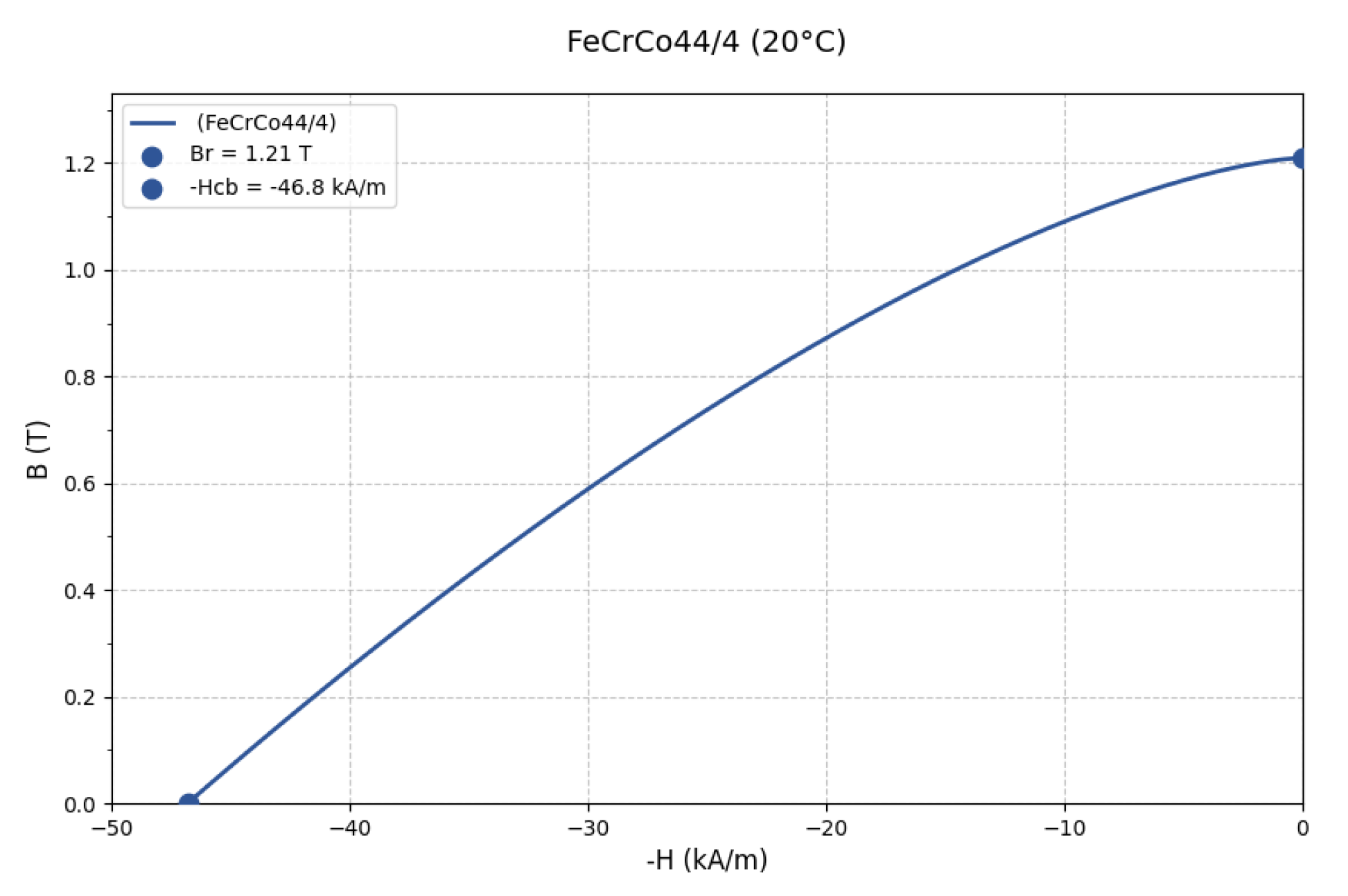
| remanent magnetism (20 °C) (T) | 1.2 |
| Scene | Method | (%) | THD (%) | Ploss (W) | tresponse (ms) |
|---|---|---|---|---|---|
| STSMO | 84.1 | 8.7 | 45.2 | 15.2 | |
| FNN-STASMO | 86.3 | 6.5 | 38.7 | 12.9 | |
| NN-STASMO | 88.9 | 4.3 | 32.1 | 9.8 | |
| STSMO | 83.4 | 9.2 | 47.8 | 16.5 | |
| FNN-STASMO | 85.1 | 7.8 | 41.2 | 13.4 | |
| NN-STASMO | 87.6 | 5.1 | 35.4 | 10.2 | |
| STSMO | 81.9 | 10.5 | 53.6 | 18.7 | |
| FNN-STASMO | 84.2 | 8.1 | 45.3 | 14.1 | |
| NN-STASMO | 86.2 | 6.8 | 39.7 | 11.5 |
| Evaluating Indicator | ILC-STASMO | FNN-STASMO | This Article SMO | Test Method |
|---|---|---|---|---|
| position error RMSE | 0.023 ± 0.005 rad | 0.017 ± 0.003 rad | 0.009 ± 0.002 rad | Tukey HSD |
| maximum overshoot | 12.7% | 8.9% | 4.2% | Welch ANOVA |
| Calculation delay | 85 μs | 120 μs | 92 μs | Kruskal-Wallis |
| Parameter sensitivity index | 0.78 | 0.65 | 0.32 | covariance analysis |
Disclaimer/Publisher’s Note: The statements, opinions and data contained in all publications are solely those of the individual author(s) and contributor(s) and not of MDPI and/or the editor(s). MDPI and/or the editor(s) disclaim responsibility for any injury to people or property resulting from any ideas, methods, instructions or products referred to in the content. |
© 2025 by the authors. Licensee MDPI, Basel, Switzerland. This article is an open access article distributed under the terms and conditions of the Creative Commons Attribution (CC BY) license (https://creativecommons.org/licenses/by/4.0/).
Share and Cite
Huang, Y.; Xie, Y.; Han, W. A Dynamic Self-Adjusting System for Permanent Magnet Synchronous Motors Using an Improved Super-Twisting Sliding Mode Observer. Sensors 2025, 25, 3623. https://doi.org/10.3390/s25123623
Huang Y, Xie Y, Han W. A Dynamic Self-Adjusting System for Permanent Magnet Synchronous Motors Using an Improved Super-Twisting Sliding Mode Observer. Sensors. 2025; 25(12):3623. https://doi.org/10.3390/s25123623
Chicago/Turabian StyleHuang, Yanguo, Yingmin Xie, and Weilong Han. 2025. "A Dynamic Self-Adjusting System for Permanent Magnet Synchronous Motors Using an Improved Super-Twisting Sliding Mode Observer" Sensors 25, no. 12: 3623. https://doi.org/10.3390/s25123623
APA StyleHuang, Y., Xie, Y., & Han, W. (2025). A Dynamic Self-Adjusting System for Permanent Magnet Synchronous Motors Using an Improved Super-Twisting Sliding Mode Observer. Sensors, 25(12), 3623. https://doi.org/10.3390/s25123623