1. Introduction
The inter-satellite link (ISL), as an integrated dynamic network between satellites and between satellites and ground stations, combines measurement and data transmission functions, bringing significant changes to the traditional operation mode of the Global Navigation Satellite System (GNSS) [
1,
2]. The primary functions of navigation ISLs can be summarized as follows: (1) achieving precise inter-satellite ranging, improving the geometric configuration of the network, and enhancing the accuracy of orbit determination and time synchronization; (2) utilizing real-time inter-satellite data transmission to increase the update frequency of navigation broadcast ephemeris; (3) enabling autonomous inter-satellite navigation in the absence of ground station support, enhancing the system’s survivability and wartime operational capabilities; (4) addressing the limitations of regional tracking station monitoring capabilities, ensuring global service performance; and (5) real-time monitoring of the integrity of navigation information, improving the system’s availability and reliability [
3,
4,
5]. Currently, major spacefaring nations are accelerating the construction and refinement of ISL systems, striving to provide higher-quality navigation service performance on a global scale [
6].
The development of the Global Positioning System (GPS) inter-satellite links began early and has reached the highest level of maturity. As early as the 1980s, the United States initiated research on ISL for the GPS, driven initially by the need for real-time monitoring of global nuclear tests and to enhance the survivability of GPS during wartime [
7]. In 1984, Ananda, M. P. et al. first proposed the fundamental framework for autonomous navigation, providing theoretical analysis results that were subsequently adopted by the U.S. military [
2]. By 1990, the theoretical design and data simulation for the GPS Block IIR ISL were completed, demonstrating that, without ground support, the user range error (URE) could be maintained below 6 m for up to 180 days [
7]. In 1997, the first GPS Block IIR satellite equipped with ISL payloads was developed, tested, and launched. Rajan et al. conducted orbit determination experiments using inter-satellite ranging data from four GPS Block IIR satellites, with results showing that the URE could be better than 3 m over 75 days [
8]. To date, GPS has launched four types of satellites: GPS IIR, GPS IIR-M, GPS IIF, and GPS III, with their corresponding operational characteristics summarized in
Table 1 [
9]. GPS satellites utilize UHF-band wide-beam antennas to establish ISLs, employing a polling-based time-division ranging system, where only one satellite transmits at any given time while the others receive [
10]. Currently, the United States is developing third-generation navigation satellites, divided into three phases: GPS IIIA, GPS IIIB, and GPS IIIC. Although GPS III was originally planned to use Ka-band (22.55–23.55 GHz) and V-band (59.3–64 GHz) frequencies, the currently launched satellites of GPS III still operate in the UHF band due to various reasons [
11]. Additionally, ongoing projects are exploring the integration of laser payloads into future GPS satellites [
12].
Facing intense competition in the global navigation arena and challenges in establishing foreign ground stations, Russia has made significant investments in developing inter-satellite link (ISL) technologies for its GLONASS system. The current implementations primarily serve GLONASS-M and GLONASS-K satellites, each demonstrating distinct technological approaches. The GLONASS-M series satellites utilize S-band wide-beam antennas to establish ISLs and employ a simplex time-division mode to measure inter-satellite pseudo-range values, achieving systematic and random errors of 0.3 m and 0.4 m, respectively [
13]. The GLONASS-K ISLs adopt a pulsed laser system, enabling centimeter-level inter-satellite ranging accuracy and medium data transmission rates (50 kbit/s), with the fastest link establishment time being less than 10 s [
14]. Looking forward, Russia’s next-generation GLONASS-K2 satellites will feature enhanced capabilities through two-phased array antennas transmitting FDMA/CDMA signals. This upgrade integrates both laser and radio frequency ISL technologies while incorporating higher-precision atomic clocks, promising substantial improvements in system performance and navigation accuracy [
15].
The Galileo navigation constellation currently does not employ ISLs, but the European Space Agency (ESA) is actively conducting exploratory research on ISL technology. In the realm of radio frequency ISLs, ESA has initiated two projects: GNSS+ and ADVISE. In the GNSS+ project demonstration, the ISLs operate in the C-band, utilizing a time-division multiple access (TDMA) ranging and communication system. This system enables bidirectional dual-frequency pseudo-range measurements between satellites, achieving an accuracy of 1–2 cm [
16]. Building on this, ESA proposed the ADVISE project, which significantly reduced payload mass and radio frequency power consumption by improving ISL design and algorithms. This solution employed a frequency-hopping time-division multiple access (FTDMA) system, achieving orbit determination accuracy of approximately 1 cm and time synchronization performance better than 0.4 ns [
17]. Simultaneously, ESA is actively exploring optical quantum links (OQLs) and laser links (Kepler), aiming to investigate new directions for ISL development and enhance the performance of navigation systems [
18].
Since the completion of the BeiDou-1 dual-satellite system at the end of 2000, China has adopted a “three-step” development strategy and officially completed the construction of the BeiDou-3 Global Navigation Satellite System (BDS-3) on 31 July 2020 [
19]. Furthermore, China plans to establish a “more ubiquitous, integrated, and intelligent” national comprehensive Positioning, Navigation, and Timing (PNT) system by around 2035 [
20,
21].
Figure 1 illustrates the development timeline of the BeiDou satellite navigation system. Between 2015 and 2016, China launched five experimental satellites (I1-S, I2-S, M1-S, M2-S, and M3-S), equipped with Ka-band ISL payloads. These satellites conducted in-orbit tests on technologies such as topology structure, communication protocols, antenna design, and autonomous navigation algorithms, achieving orbit determination accuracy better than 2 m [
22]. Starting in 2017, BDS-3 satellites began carrying ISL payloads to enable inter-satellite measurement and communication. By December 2018, the initial BDS-3 constellation was successfully established, consisting of 18 Medium Earth Orbit (MEO) satellites and 1 Geostationary Earth Orbit (GEO) satellite [
23]. Guo et al. processed 30 days of ISL measurement data from 18 MEO satellites using a distributed approach based on the extended Kalman filter, demonstrating that the three-dimensional orbital error could be less than 2.30 m over 30 days [
24]. Xie et al. analyzed the orbit determination performance of 18 MEO satellites and 1 GEO satellite using 43 days of ISL measurement data from 2019. The results showed that the radial orbit error of the MEO satellites was on the order of 2–4 cm, while that of the GEO satellite was on the order of 8–10 cm [
25].
Currently, all BDS-3 satellites are equipped with Ka-band ISL payloads, enabling precise orbit determination and time synchronization through inter-satellite precision measurement and data transmission. Zhang et al. analyzed the inter-satellite ranging performance using 30 days of measurement data from the complete BDS-3 constellation, revealing that the ISL ranging accuracy was better than 5 cm [
26]. Guo et al. conducted an experimental analysis using one month of raw observation data from 29 BDS-3 satellites, consistently demonstrating that the time synchronization accuracy of each satellite was better than 0.4 ns [
6]. The BeiDou ISL communication and measurement system employs a time-division half-duplex mode, establishing narrow-beam directional links based on a phased-array mechanism. Each satellite, following a time-slot schedule uploaded from the ground, establishes links with other satellites (or ground anchor stations) in a polling manner. The BDS-3 ISL system divides the timeline into superframes (1 min), with each superframe further subdivided into 20 time slots (3 s). Within a single time slot, the linked satellites alternately transmit signals to each other during their respective 1.5 s intervals, completing two-way inter-satellite measurement and communication [
26,
27,
28].
Currently, ISLs in major global navigation systems predominantly employ a time-division half-duplex (TDHD) mode. While numerous scholars have focused on analyzing link performance based on raw inter-satellite observation data, such as orbit determination accuracy, time synchronization precision, and routing transmission efficiency, research on the operational mechanisms of ISLs remains limited. The TDHD mode, which prevents simultaneous transmission and reception on the same frequency, results in unidirectional transmission rates being only 50% of the total channel capacity. Additionally, the link establishment process is complex, and timestamp calculation and error correction are prone to significant inaccuracies. These limitations lead to issues such as low communication efficiency, high latency, and restricted inter-satellite measurement accuracy [
3]. In contrast, Co-frequency Co-time Full Duplex (CCFD) technology, a key innovation proposed during the 5G era, has matured significantly in recent years [
29,
30,
31]. Compared to traditional time-division and frequency-division systems, CCFD technology enables wireless devices to achieve simultaneous signal transmission and reception on the same frequency. Relative to time-division systems, CCFD technology allows concurrent signal transmission and reception, theoretically doubling the information throughput within the same time interval. In contrast to frequency-division systems, CCFD technology can effectively conserve bandwidth resources, theoretically improving spectral efficiency by a factor of two. Currently, numerous researchers have begun dedicating efforts to the study of CCFD technology, covering a wide range of fields such as massive multiple-input multiple-output systems, low-power wide-area networks, relay communication networks, Wi-Fi systems, Long-Term Evolution systems, and cognitive radio [
29]. Introducing CCFD into ISL measurement and communication processes could effectively overcome the constraints of TDHD systems, which are unable to simultaneously transmit and receive signals on the same frequency. Moreover, it would simplify the link establishment process and enable continuous inter-satellite transmission and precise measurement. In terms of transmission, CCFD could double the inter-satellite transmission rate, measurement frequency, and data update rate. For measurement, CCFD could effectively mitigate ranging errors caused by relative motion, clock bias, and Doppler effects between satellites. This would eliminate the need for complex models to improve ranging accuracy and enhance the performance of inter-satellite measurements.
In this paper, we propose a novel inter-satellite two-way measurement method based on the CCFD system to enhance the overall performance of the ISL network.
Section 2 analyzes the self-interference suppression performance of the CCFD system from three domains and presents the current total self-interference suppression level.
Section 3 provides a detailed analysis of the spatial configuration of the BDS-3 satellite navigation constellation, constructing a dynamic link constraint model based on satellite visibility and antenna directivity.
Section 4 conducts a comprehensive link budget analysis of the BDS-3 ISL.
Section 5 systematically introduces the proposed two-way measurement method for ISL, including the fundamental principle, system model, and key errors, theoretically evaluating the system performance under the new framework.
Section 6 presents experimental simulations and analyses, autonomously constructing a BDS-3 ISL scenario and a digital simulation verification platform to capture inter-satellite topological characteristics, validate the feasibility of the full-duplex system, and analyze pseudo-code ranging performance under the new framework.
Section 7 analyzes the experimental results and discusses potential directions for future research.
Section 8 provides a comprehensive summary and synthesis of the research findings presented in this paper.
3. BDS-3 Constellation Configuration and ISL Establishment Constraints
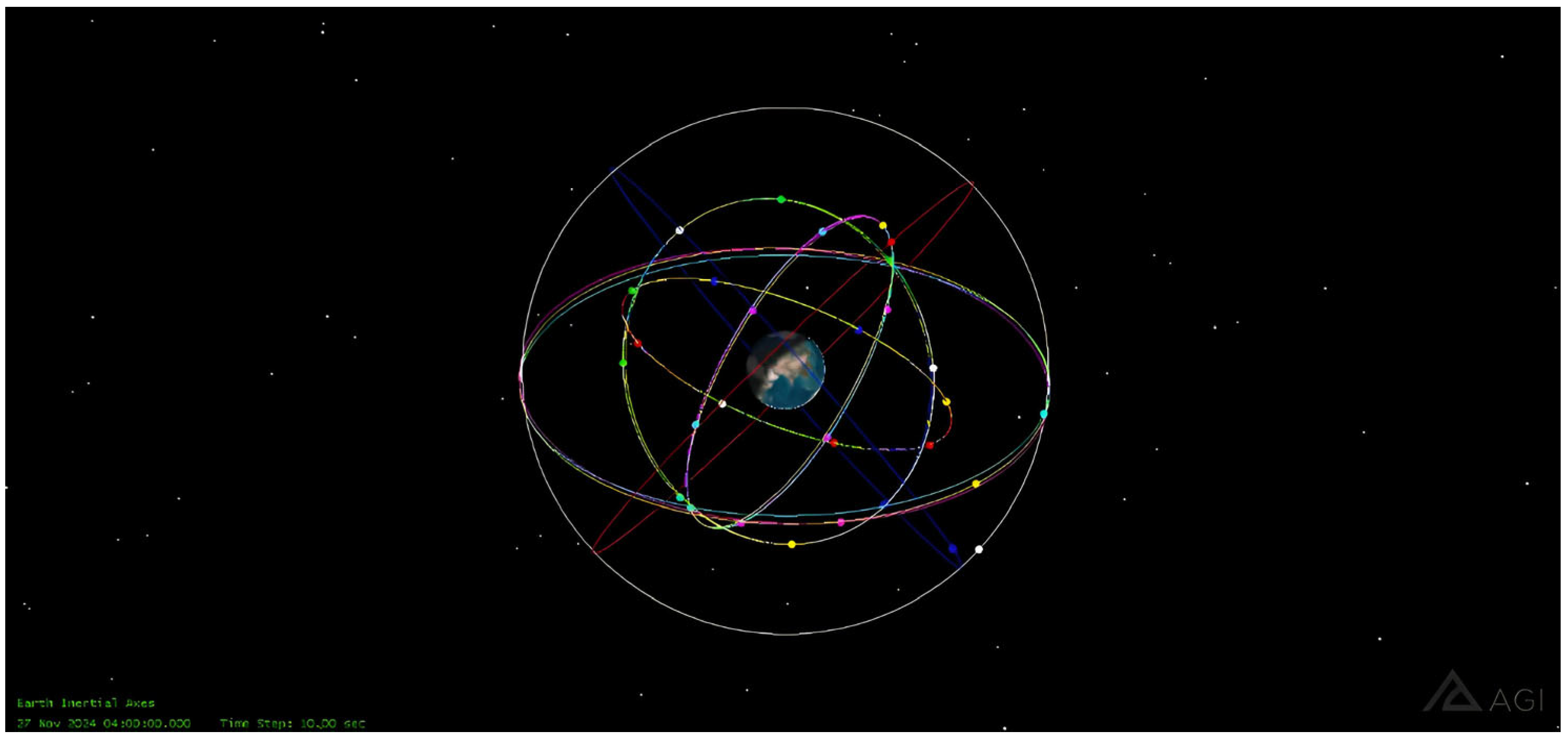
The BDS-3 constellation is a multi-layered heterogeneous hybrid system, consisting of 3 GEO satellites, 3 Inclined Geosynchronous Orbit (IGSO) satellites, and 24 MEO satellites. The MEO satellites are arranged in a Walker 24/3/1 constellation configuration, featuring an orbital altitude of 21,528 km and an inclination of 55°. This configuration distributes the 24 MEO satellites across three evenly spaced orbital planes, with eight satellites uniformly positioned within each plane. Additionally, the phase difference between corresponding satellites in adjacent orbital planes is 15°. For the 24 MEO satellites configured in the Walker constellation, the satellites within the three orbital planes are labeled as MEO1m, MEO2n, and MEO3k, where m, n, k = 1, 2, …, 8. The 3 IGSO satellites have an inclination angle of 55° and a theoretical orbital altitude of 35,786 km. The 3 GEO satellites are positioned at longitudes of 80° E, 110.5° E, and 140° E, with a theoretical orbital altitude of 35,786 km.
The BDS-3 constellation features a large number of orbital planes and complex orbital types, and the relative positions and spatial relationships between satellites change rapidly over time. Therefore, the following constraints must be considered when establishing ISLs.
3.1. Satellite Visibility Constraints
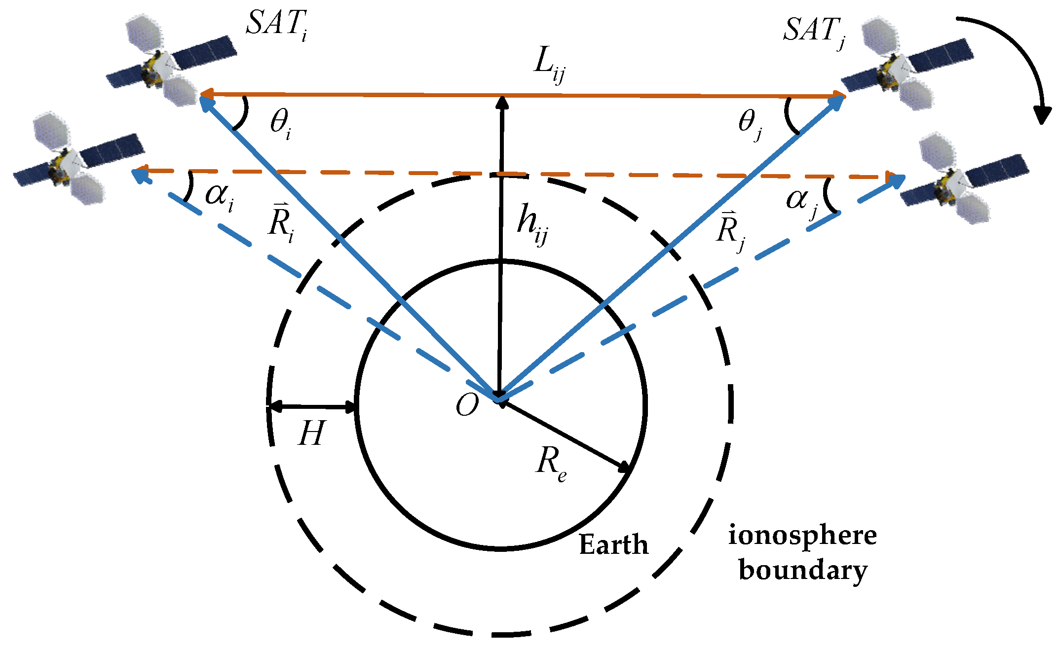
The fundamental condition for establishing a link between two satellites is that they are mutually visible in space, meaning there is no Earth obstruction between them. Additionally, to avoid interference and effects from the troposphere and ionosphere on the ISL signals, the visibility constraint can be strengthened by requiring that the inter-satellite communication zone be at least 1000 km above the Earth’s surface.
As shown in
Figure 4,
SATi and
SATj represent the two satellites establishing the link,
O denotes the center of the Earth,
is the Earth’s radius, and
is the height of the ionosphere. The vectors
and
represent the direction vectors from the Earth’s center to satellites
i and
j, respectively.
is the distance between the two satellites,
is the distance from the Earth’s center to the line connecting satellites
i and
j,
is the angle between the line connecting satellite
i to satellite
j and the line connecting satellite
i to the Earth’s center, and
is the angle between the line connecting satellite
j to satellite
i and the line connecting satellite
j to the Earth’s center.
and
are Earth occlusion angles of satellites
i and
j.
To ensure unobstructed inter-satellite signal transmission and guaranteed communication quality, the spatial positional relationship between satellite
i and satellite
j must satisfy the following equation:
Using
and
to represent
, the distance constraint formula for inter-satellite visibility can be derived as follows:
When the line connecting satellite
i and satellite
j is tangent to the ionosphere boundary, the angle between the satellite connection line and the line from the satellite to the Earth’s center can be calculated, resulting in the angle constraint formula for inter-satellite visibility:
3.2. Antenna Directivity Constraints
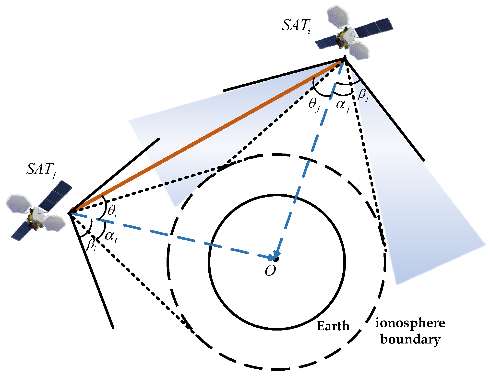
The BDS-3 employs phased-array antennas for its ISLs. By controlling the phase relationships of the antenna elements, the system can achieve beam scanning over a wide spatial range, enabling effective signal transmission. The BDS-3 ISLs operate in the Ka-band, which features relatively narrow antenna beams. By adjusting the beam direction, the system can establish point-to-point signal transmission links. Furthermore, phased-array antennas have a maximum beam scanning angle. Therefore, when establishing ISLs, the antenna directivity constraints must be considered. Specifically, the satellite pair planning to establish a link must simultaneously fall within each other’s beam scanning range to ensure effective link establishment.
Figure 5 illustrates the antenna directivity constraints, where
and
represent the maximum beam scanning ranges of satellite
i and satellite
j, respectively. If both satellites are within each other’s visibility range, the following antenna directivity constraint conditions must be satisfied, as expressed in the equation below:
Considering practical engineering constraints, the maximum beam scanning range for BDS-3 can be set to 60° [
25]. Taking into account both satellite visibility and antenna directivity constraints, a theoretical analysis of the ISL antenna scanning range and the maximum communication distance can be conducted. For MEO-MEO type links and MEO-GEO/IGSO type links, the maximum communication distance can be calculated as follows:
where
represents the maximum inter-satellite distance for MEO-MEO type links, and
represents the maximum inter-satellite distance for MEO-GEO/IGSO type links.
denotes the theoretical orbital altitude of MEO satellites, and
denotes the theoretical orbital altitude of GEO/IGSO satellites. The Earth occlusion angles for MEO satellites and GEO/IGSO satellites can be calculated using the following equations:
where
represents the Earth occlusion angle for MEO satellites, and
represents the Earth occlusion angle for GEO/IGSO satellites. Taking
= 6378 km,
= 1000 km,
= 21,528 km, and
= 35,786 km, and substituting these values into Equations (5)~(8), the maximum inter-satellite communication distance and the Earth occlusion angle can be calculated. The calculation results are shown in
Table 5.
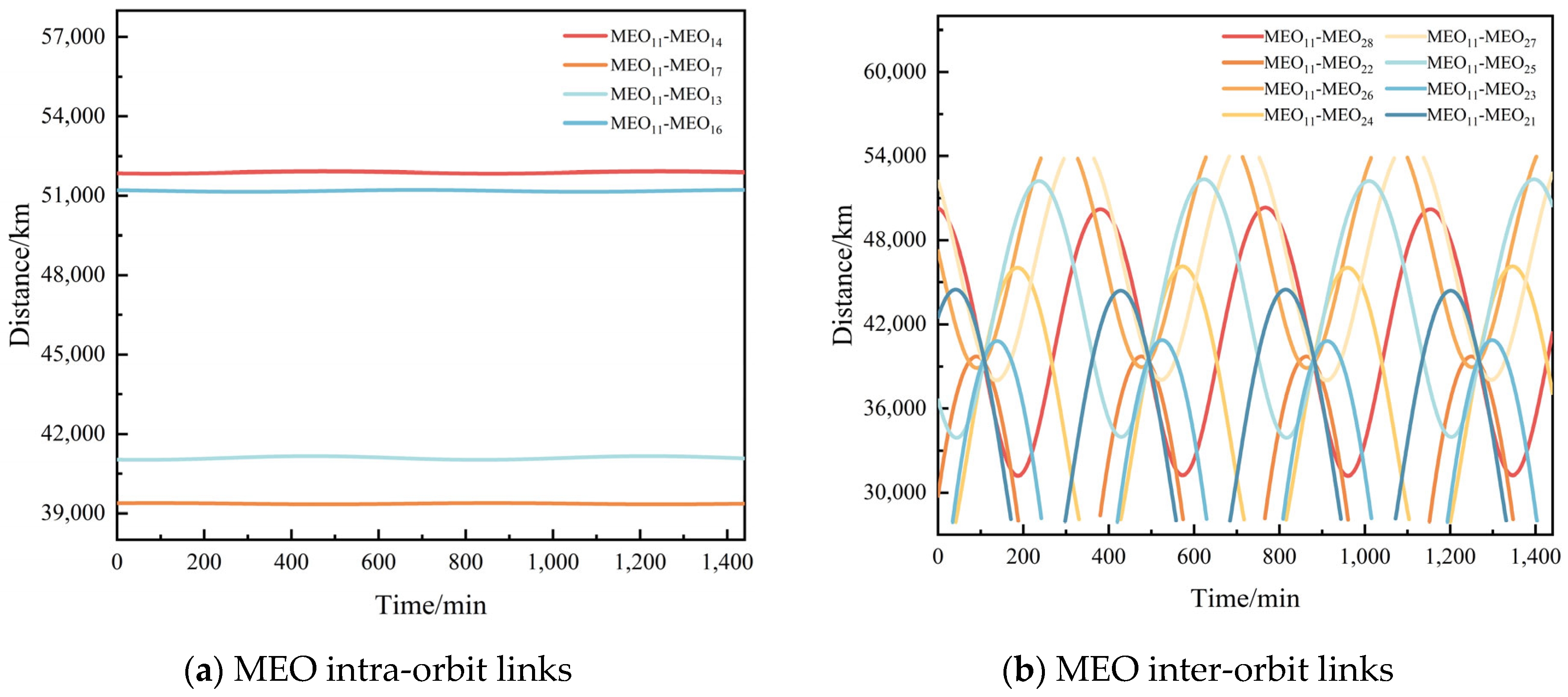
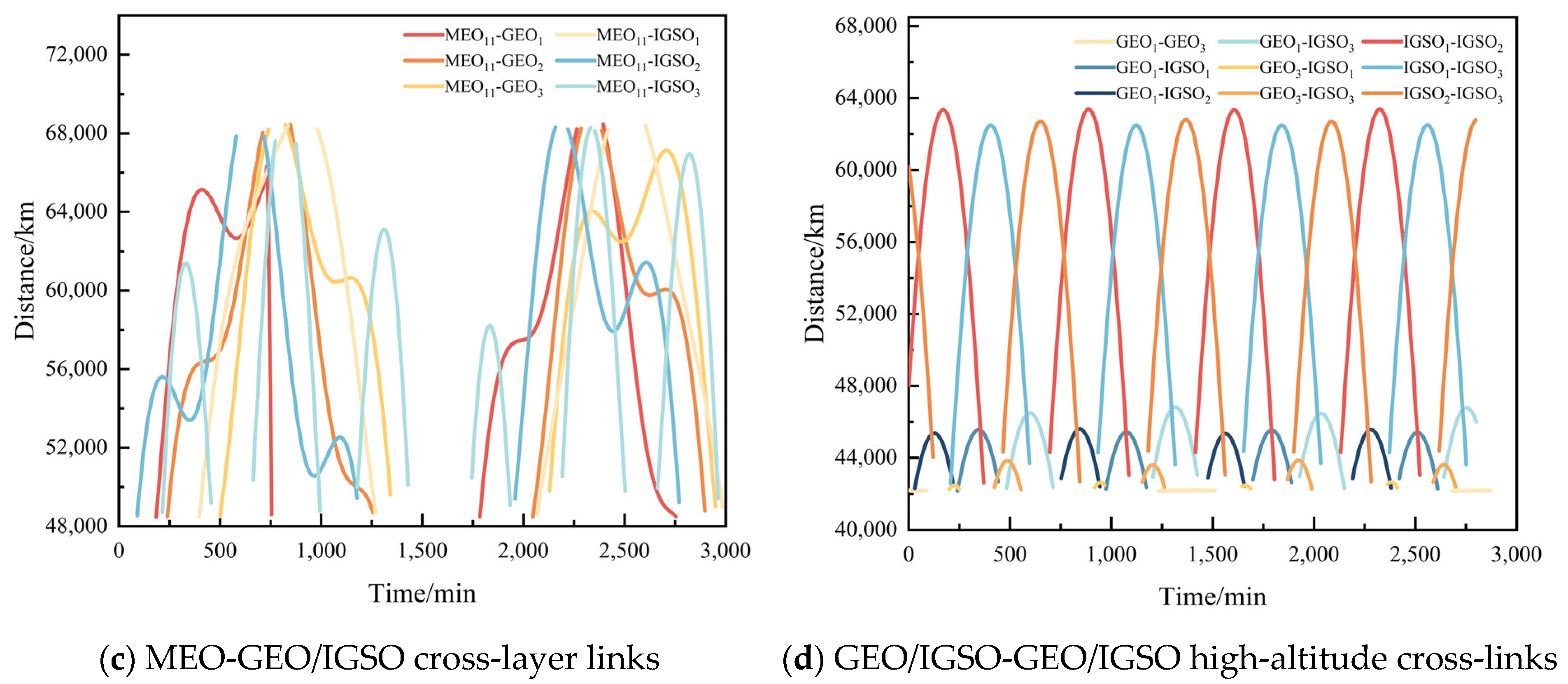
Simulation results indicate that the maximum inter-satellite communication distance for MEO-MEO type links can reach 55,897.12 km, while for MEO-GEO/IGSO type links, it can reach 70,477.33 km. The Earth occlusion angles for MEO satellites and GEO/IGSO satellites are 14.79° and 9.84°, respectively. In the next step of inter-satellite topology analysis, inter-satellite visibility and antenna directivity constraints should be considered. To ensure signal transmission quality with a sufficient margin, the beam scanning range for MEO satellites can be set to [15°, 60°], while for GEO/IGSO satellites, it can be set to [10°, 60°].
5. Two-Way Measurement Method in CCFD
Introducing CCFD into the BDS-3 ISL system enables simultaneous transmission and reception of signals on the same frequency, thereby enhancing the overall performance of the constellation. This section provides a detailed analysis of the fundamental principle, system model, and key errors of inter-satellite two-way measurement in CCFD. It has been proved in theory that this approach can achieve higher ranging precision.
5.1. Principle of Two-Way Measurement Method in CCFD
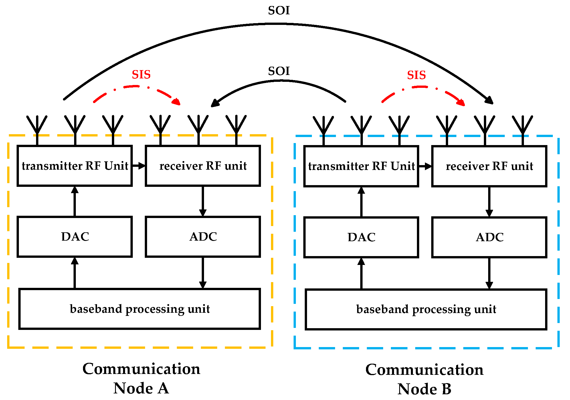
The two-way measurement method in CCFD is described as follows: (1) In terms of the time slot schedule uploaded from the ground, the satellite pair is identified to establish the link. (2) The two satellites (satellite and ) agree on the same transmission time and simultaneously send signals to each other. The signals share the same frame structure, with the baseband clock and carrier frequency generated locally by each satellite. (3) While transmitting, each satellite synchronously receives the signal sent by the other satellite. (4) Through spatial-domain, RF-domain, and digital-domain self-interference suppression, the self-interference signal can be reduced to the receiver noise floor, enabling effective signal reception. (5) The satellites execute signal acquisition, tracking, and demodulation processes to recover the information frame, extract the transmission epoch time, and integrate it with the local epoch time to compute the local pseudo-range. (6) The local pseudo-range is embedded into the information frame and transmitted to the other satellite. Both satellites then construct the two-way observation equation using the local pseudo-range and the pseudo-range demodulated from the received information frame. (7) The system performs timestamp calculation and key error correction to derive the modified pseudo-range equation. (8) The system performs summation and difference operations on the modified pseudo-range equation to derive the inter-satellite geometric distance and clock bias, which are necessary for precise orbit determination and time synchronization.
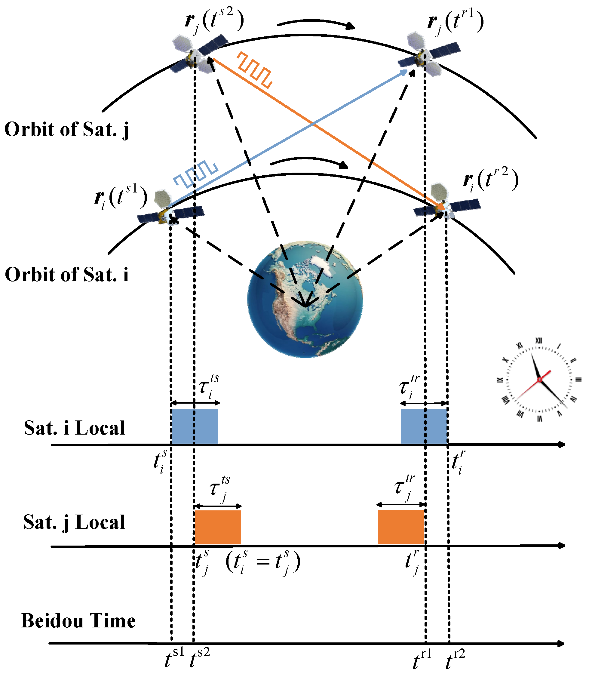
Figure 6 illustrates the timing diagram of inter-satellite two-way measurement in CCFD, with the following parameter definitions: (1)
is the local transmission time of the satellite
, and
is the corresponding BeiDou time (BDT).
is the local transmission time of the satellite
, and
is the corresponding BDT. (2)
is the local reception time of the satellite
, and
is the corresponding BDT.
is the local transmission time of the satellite
, and
is the corresponding BDT. (3)
and
represent the transmission and reception channel delays of the satellite
, respectively.
and
represent the satellite’s transmission and reception channel delays
, respectively. (4)
and
denote the position vectors of the satellite
in the Earth-Centered Inertial (ECI) coordinate system at the transmission and reception times, respectively.
and
denote the position vectors of the satellite
in the ECI coordinate system at the transmission and reception times, respectively.
5.2. System Model of Two-Way Measurement Method in CCFD
Based on the process of inter-satellite two-way measurement, the observation equation can be derived as follows:
where
and
represent the locally measured pseudo-ranges of satellites
and
, respectively.
and
are the clock bias between the local time of the satellite
and BDT at times
and
, respectively.
and
are the clock bias between the local time of the satellite
and BDT at times
and
, respectively. The clock bias can be expressed as follows:
and
represent the systematic errors of the two-way measurement, while
and
denote the ranging noise. The systematic errors can be further expressed as follows:
where
and
represent the gravitational time delay of the two-way measurement, respectively.
and
denote the time delay of periodic relativistic effects in the two-way measurement, respectively.
and
represent the time delay of phase center offset (PCO) in the two-way measurement, respectively. Therefore, the inter-satellite two-way observation equation can be expressed in detail as follows:
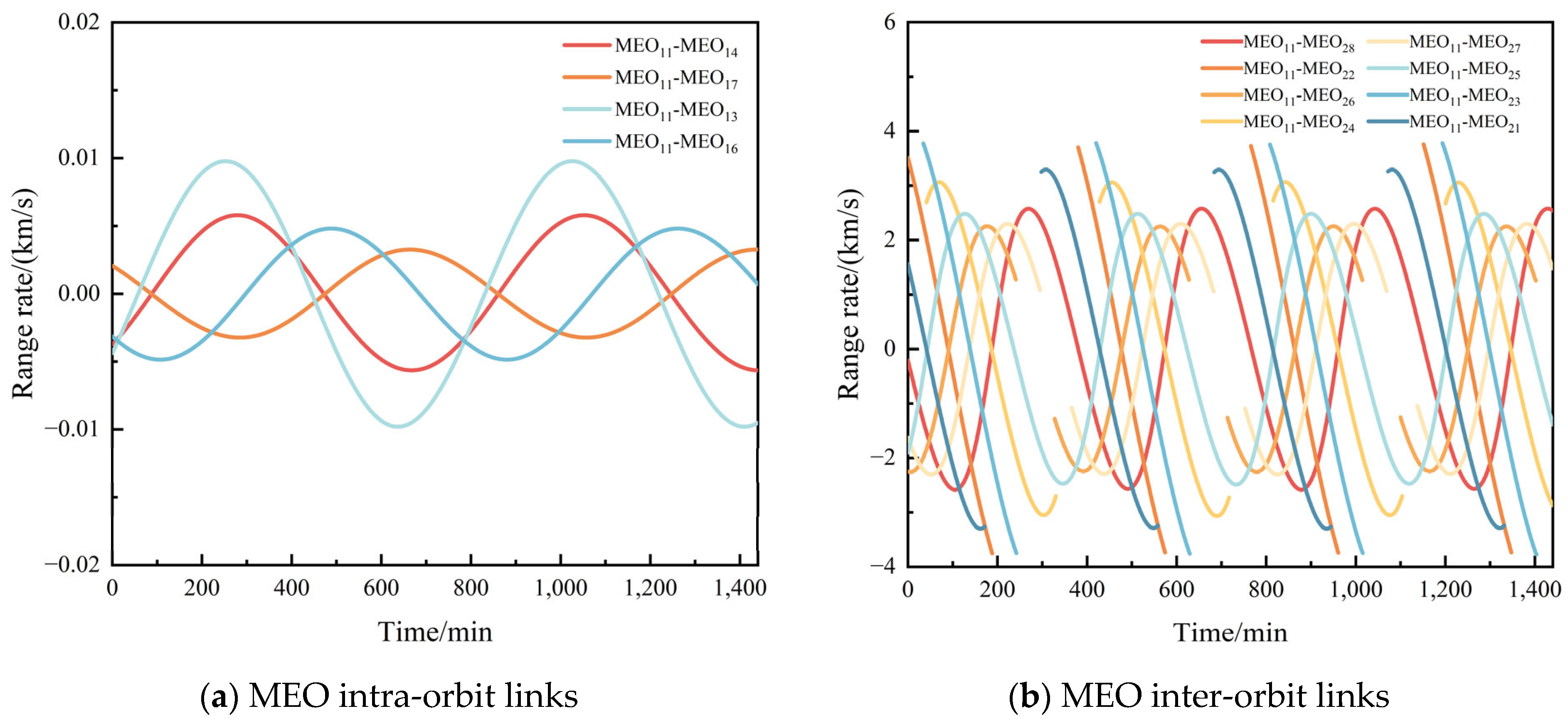
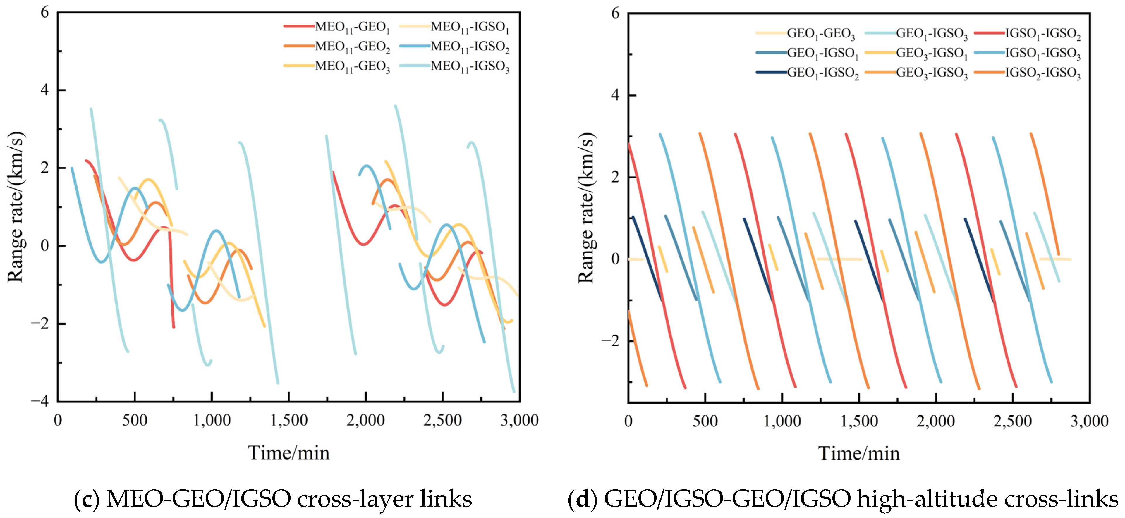
Given that the maximum communication distance of BDS-3 ISLs can reach 70,000 km and the relative velocity between satellites can reach several km/s, the effects of signal propagation delay and high-speed satellite motion cannot be overlooked [
65]. ISL ranging aims to determine the geometric distance between two satellites at the same instant. Therefore, it is necessary to perform timestamp calculations on the observations to align the inter-satellite pseudo-range measurement to a unified system time.
can be selected as the reckoning time (
) in CCFD, and the inter-satellite two-way observation equation can be adjusted as follows:
where
and
are the distance corrections for the inter-satellite two-way measurement, respectively.
is the clock bias correction for satellite
from time
to
, and
is the clock bias correction for satellite
from time
to
. Comparing Equations (25) and (26), the following equations can be derived as follows:
Analyzing the measurement process from satellite
to satellite
, it can be concluded that:
where
represents the velocity of satellite
, and
denotes the unit direction vector from satellite
to satellite
. Let
, and perform a first-order Taylor expansion at
, yielding as follows:
where
where
is a value between
and
. Since the velocity of the satellite changes slowly during a single ranging process and the linked satellites are tens of thousands of kilometers apart, the acceleration of the satellite and the rate of change of the inter-satellite direction can be approximated as zero over a short period, and
can be neglected. Letting
, Equation (30) can be written as follows:
Substituting Equation (32) into Equation (29), it can be concluded that:
For the measurement process from satellite
to satellite
, we can similarly derive the following result:
where
represents the velocity of the satellite
, and
denotes the unit direction vector from satellite
to satellite
. Substituting Equations (33) and (34) into Equation (27), the following expressions can be obtained as follows:
Let
, representing the spatial distance between satellites at different times. A first-order Taylor expansion of
at time
is performed. Since the duration of a single two-way measurement is short, the inter-satellite acceleration can be approximated as zero [
3], allowing the Taylor expansion remainder term to be neglected. The expansion of
and Equation (36) can be expressed as follows:
To better describe the calculation error, we can define it as follows:
where
is the “spatial reckoning” term resulting from the difference between transmission and reckoning times.
and
are the “dynamic compensation” terms caused by the high-speed motion of the satellites. Therefore, the distance correction term for the inter-satellite two-way measurement can be rewritten as follows:
Under the monitoring and control of ground stations, the clock bias between BeiDou satellite local time and BDT generally does not exceed 1 ms [
3]. Therefore, the clock bias between satellites is typically maintained within 2 ms. The following relationship can be obtained as follows:
As a navigation satellite, it stores its own broadcast ephemeris and the almanac of other satellites in the constellation. The precision of calculating satellite velocity using the broadcast ephemeris is 0.1 mm/s, while using the almanac yields a precision of dm/s [
66]. Therefore, after calculating with the satellite’s local ephemeris and almanac, the correction precision of
can reach the sub-millimeter level, and the correction error can be considered negligible.
For the TDHD system, the reckoning time is often chosen at the midpoint of the two-way link transmission period. For a 3 s time slot, the difference between the reckoning time and the transmission time is approximately 0.75 s. In this case, the correction precision of the “spatial reckoning” term is only at the centimeter level, which does not meet the high-precision ranging requirements for ISLs. The CCFD system can effectively overcome this issue.
For the “dynamic compensation” term, since the maximum inter-satellite communication distance can reach 70,000 km, the maximum inter-satellite transmission delay is approximately 0.23 s, which means as follows:
According to Equation (39), the “dynamic compensation” term depends on the receiving satellite’s velocity (which can be calculated from ephemeris data with an accuracy of 0.1 mm/s), the inter-satellite unit direction vector, and the transmission time interval. Since the maximum inter-satellite communication duration is approximately 0.23 s and the inter-satellite distance can extend to tens of thousands of kilometers, the unit direction vector between satellites remains effectively constant during a single transmission slot. Consequently, the “dynamic compensation” term can be corrected to an order of 10−2 mm, rendering it negligible in practice.
For the clock bias correction term, since the frequency stability of onboard atomic clocks is generally better than 10
−13 s/s [
25], and the difference between the two-way transmission/reception times and the reckoning time is no more than 0.5 s in CCFD, the maximum value of the clock bias correction term is only on the order of 10
−14 s, corresponding to a distance on the order of 10
−3 mm, which is negligible.
In summary, the analysis shows that the error introduced by timestamp reckoning in CCFD is primarily caused by the “dynamic compensation” term in the distance correction. After ephemeris and almanac correction, the precision can reach the sub-millimeter level. Compared to the traditional TDHD system, the correction precision is significantly improved, meeting the requirements for high-precision inter-satellite measurement.
5.3. Key Errors of the Two-Way Measurement Method in CCFD
During the process of inter-satellite two-way measurement, various types of errors exist, including channel time delay, gravitational time delay, the time delay of periodic relativistic effects, the time delay of PCO, and ranging noise. The presence of these errors can significantly impact the precision of inter-satellite measurements, necessitating their calculation and compensation.
5.3.1. Channel Time Delay
Channel delay error is one of the significant error terms affecting the precision of inter-satellite measurements. Due to the presence of various nonlinear components in the equipment, along with the effects of aging and temperature drift, the channel delay of the transceiver equipment can vary over time. For a single measurement, since the measurement duration is short and the equipment state changes minimally, the channel delay can be assumed to be constant.
Since the system employs the CCFD framework, allowing simultaneous transmission and reception of signals on the same frequency, an online calibration method can be used to perform real-time calibration of the channel delay. By introducing a self-calibration channel into the ranging equipment, a closed-loop circuit is formed between the transmission and reception channels. Through transmission–reception switching, three different delay combinations are obtained, and the transmission and reception equipment delays can be calculated, achieving a calibration precision better than 0.3 ns [
66].
5.3.2. Gravitational Time Delay
Due to the effects of general relativity, gravitational time delay errors occur during signal transmission. These errors can be calculated and corrected using the following formula [
6]:
where
is the post-Newtonian parameter, and
is the Earth’s gravitational constant.
5.3.3. Time Delay of Periodic Relativistic Effects
Under the influence of special relativity, satellite clocks exhibit a nominal frequency offset (NFO) and periodic relativistic effects. The NFO can be eliminated by adjusting the clock frequency before transmission, and the correction formula can be expressed as follows [
67]:
where
is the NFO in Hz, and
is the satellite orbit semi-long axis in m. The periodic relativistic effects can be calculated and corrected using the following formula [
68]:
5.3.4. Time Delay of PCO
Inter-satellite measurements are based on the phase center of the transceiver antenna, while the antenna is installed based on its geometric center. During the measurement process, the inconsistency between the antenna’s phase center and its geometric center introduces an error known as the time delay of PCO.
The time delay of PCO can be corrected by the factory default values, which were calibrated by the satellite manufacturer and have been released on the Beidou official website [
69]. Alternatively, it can be determined through in-orbit calibration. This method generally utilizes the observation data between the globally uniformly distributed ground stations and the satellites and solves the antenna phase center deviation parameters through network estimation [
70].
5.3.5. Ranging Noise
The inter-satellite pseudo-range values
and
are extracted from the pseudo-code tracking loop of the satellite receiving device. The precision of pseudo-range measurements is related to the thermal noise error and dynamic stress error of the tracking loop. The 1σ tracking error of the pseudo-code loop can be expressed as follows:
where
is the tracking error caused by thermal noise, and
is the dynamic stress error caused by inter-satellite relative movement.
can be expressed in the following form as follows:
where
is the order of the loop, and
is the natural frequency in Hz. During actual tracking, carrier-aided code tracking technology is often used, which can largely eliminate most of the dynamic stress errors. Therefore, dynamic stress errors can be neglected, and the ranging error is primarily caused by thermal noise.
can be expressed as follows:
where
is the pseudo-code rate in Hz,
is the equivalent noise band of the code loop in Hz,
is the correlation interval, and
is the coherent integration time. When the inter-satellite ranging system uses the CCFD scheme, compared to the traditional TDHD scheme, the measurement time can be doubled, and the system can reduce the equivalent noise band
, achieving higher-ranging accuracy by sacrificing convergence speed. Therefore, it can be theoretically verified that using the CCFD scheme can effectively reduce the pseudo-code ranging noise.
7. Discussion
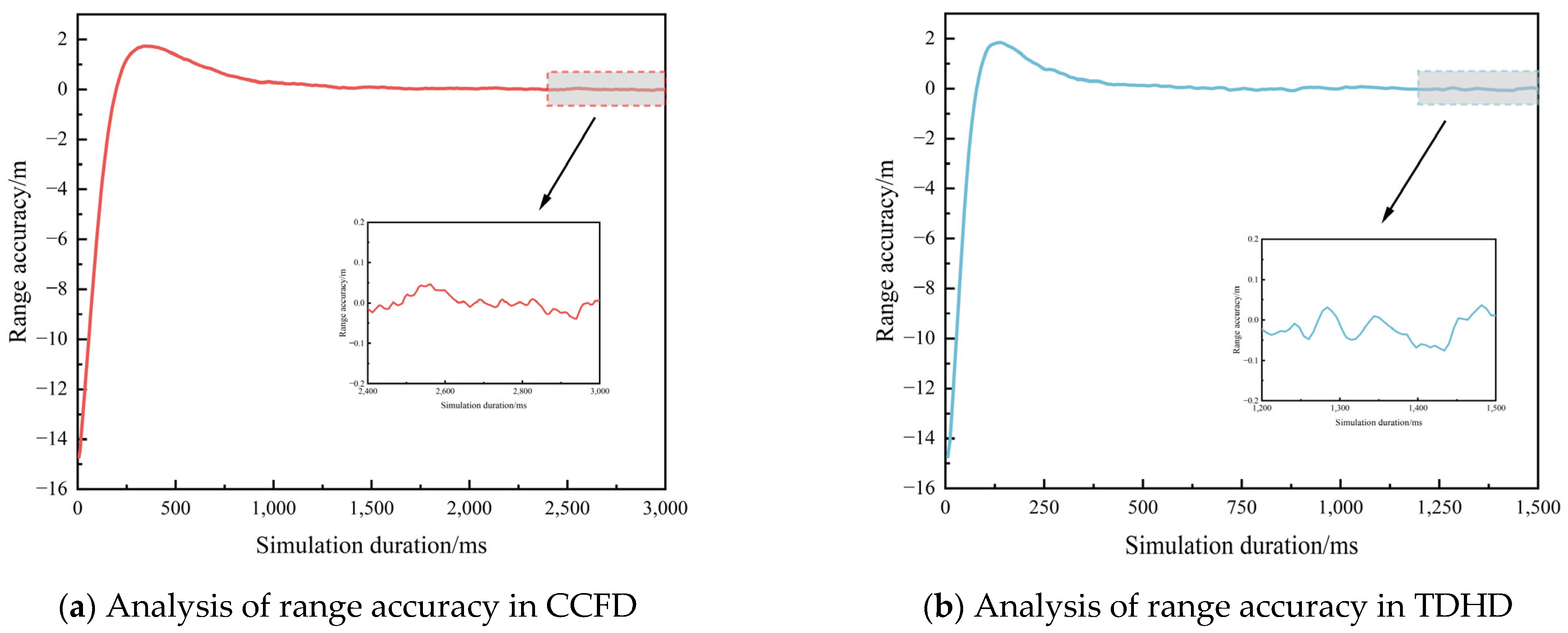
Theoretical analysis and experimental simulations confirm that the CCFD scheme can significantly enhance inter-satellite ranging accuracy, with its technical advantages manifested in two key aspects: Firstly, regarding observation precision, the CCFD scheme doubles the inter-satellite measurement duration, allowing the system to achieve narrower code loop equivalent noise bandwidth at the cost of moderately reduced loop convergence speed, thereby markedly improving pseudo-range observation accuracy (with improvement exceeding 50%). Secondly, in terms of timestamp reckoning, the CCFD system can effectively eliminate the “spatial reckoning” errors inherent in the conventional TDHD system caused by the difference between transmission and reckoning timestamps. After ephemeris and almanac corrections, residual errors can be maintained at negligible levels.
As a critical metric for BDS-3 ISL construction, ranging accuracy directly impacts system performance. Given that both orbit determination and clock offset calibration rely on pseudo-range observations, accuracy improvement is essential for achieving sub-meter precise orbit determination and nanosecond-level time synchronization, which will significantly enhance the navigation system’s service quality and constellation autonomy.
It is noteworthy that CCFD technology has applications extending far beyond BDS-3 ISLs. It demonstrates considerable potential in large-scale heterogeneous constellation networking, satellite formation flying, space station TT&C, and new technology demonstration satellites. While this study focuses on optimizing pseudo-code ranging methods, CCFD’s unique long-duration measurement capability creates opportunities for implementing higher-accuracy techniques (such as carrier-phase-smoothed pseudo-range and pure carrier-phase ranging), which will constitute our primary research direction. Furthermore, CCFD implementation not only enhances measurement performance but also improves inter-satellite data transmission efficiency and routing reliability; these derivative advantages warrant further investigation.

 and
and 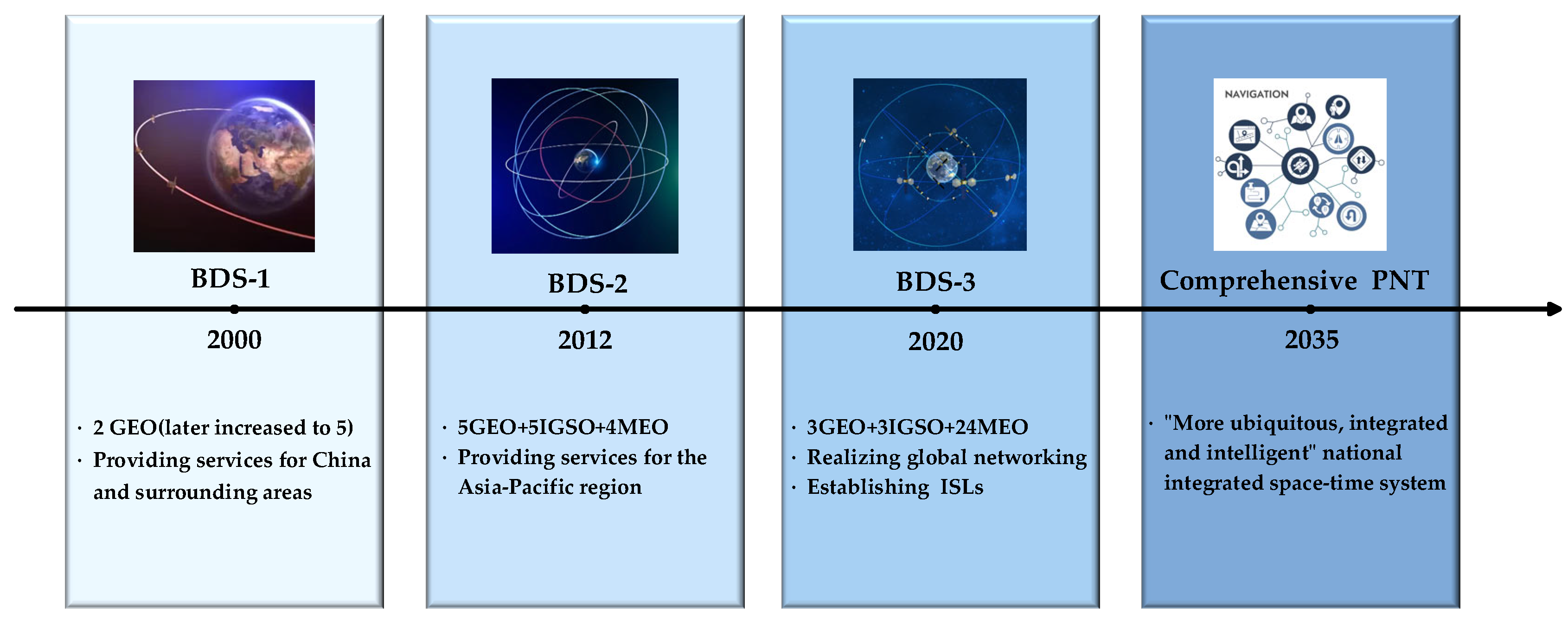


