
An Effective Method for Calculation of Mutual Inductance Between Rectangular Coils at Arbitrary Positions in Space


 ,
,
Abstract

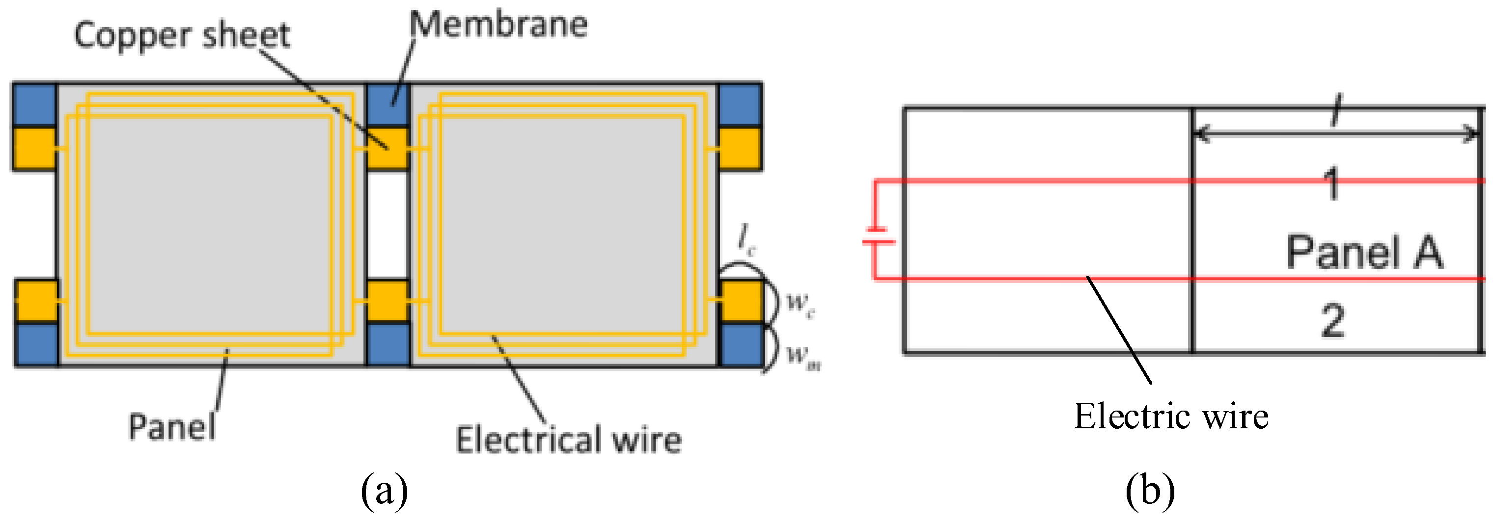
1. Introduction
2. Mutual Inductance Calculation of Rectangular Coil
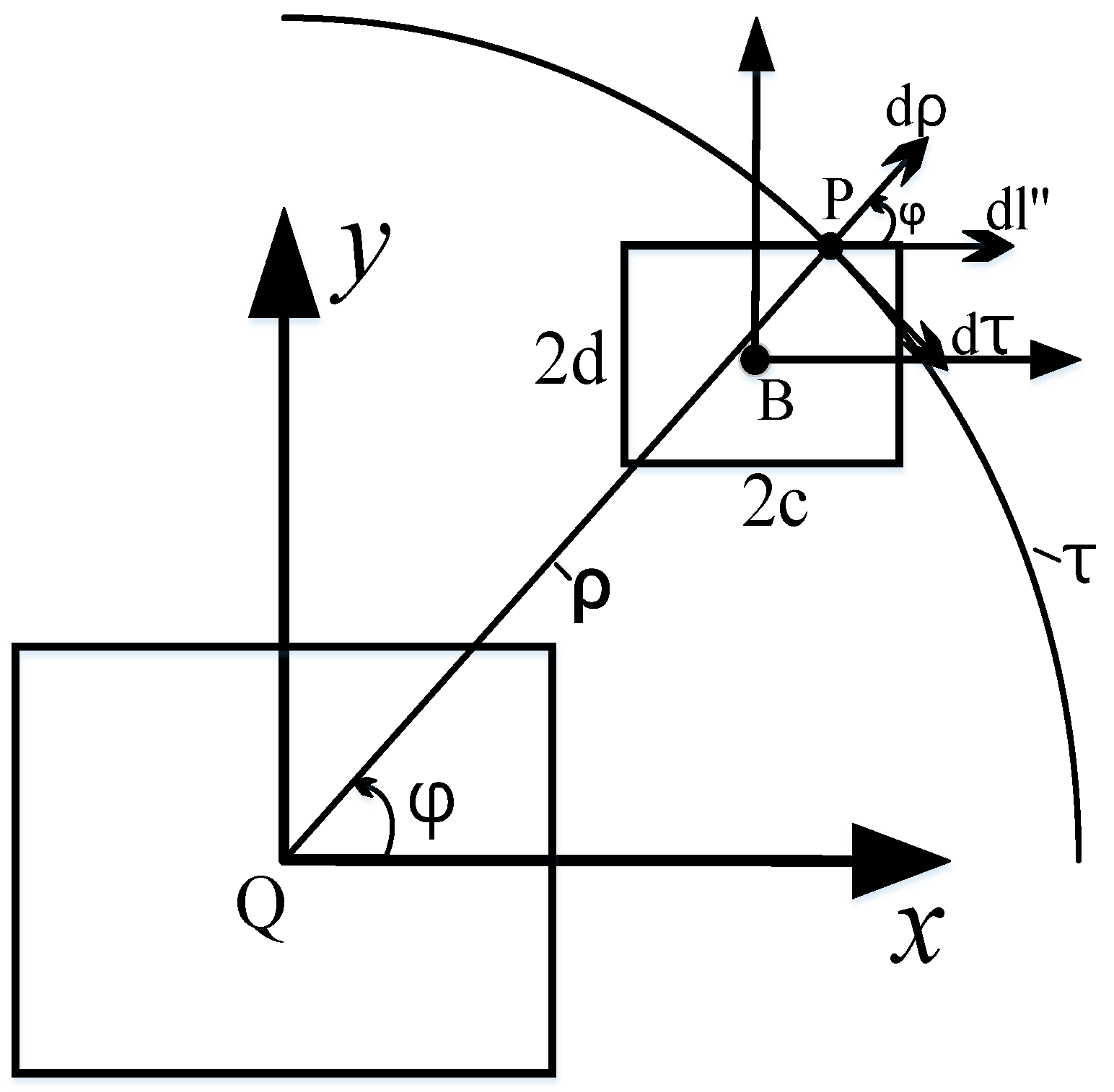
2.1. Coordinate Transformation
2.2. Neumann Formula
2.3. Mutual Inductance Calculation
3. Algorithm Verification
3.1. Calculation of Vertical Offset Mutual Inductance
- (1)
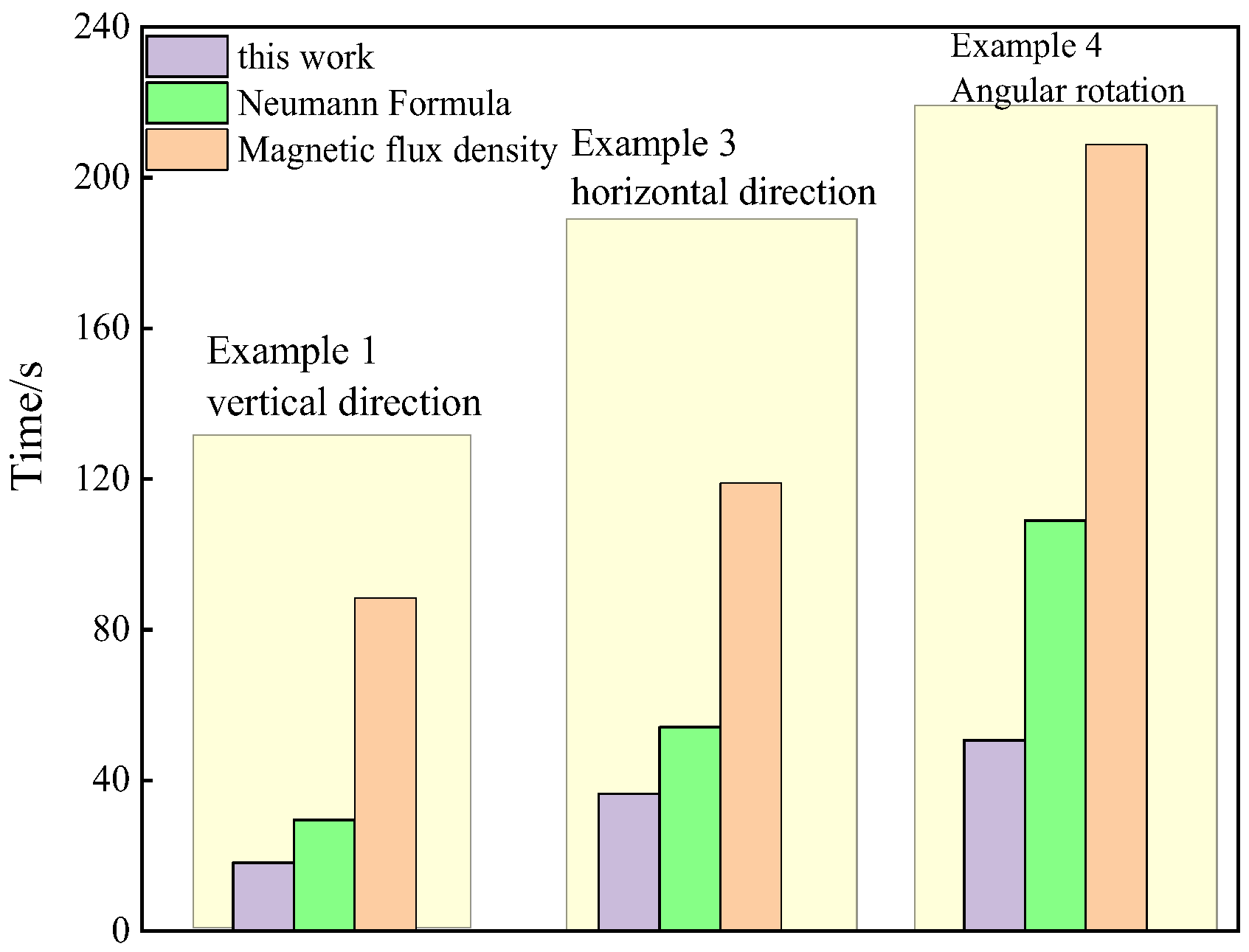
- Example 1
3.2. Calculation of Horizontal Offset Mutual Inductance
- (1)
- Example 2
- (2)
- Example 3
3.3. Mutual Inductance Calculation at Arbitrary Position in Space
- (1)
- Example 4
- (2)
- Example 5
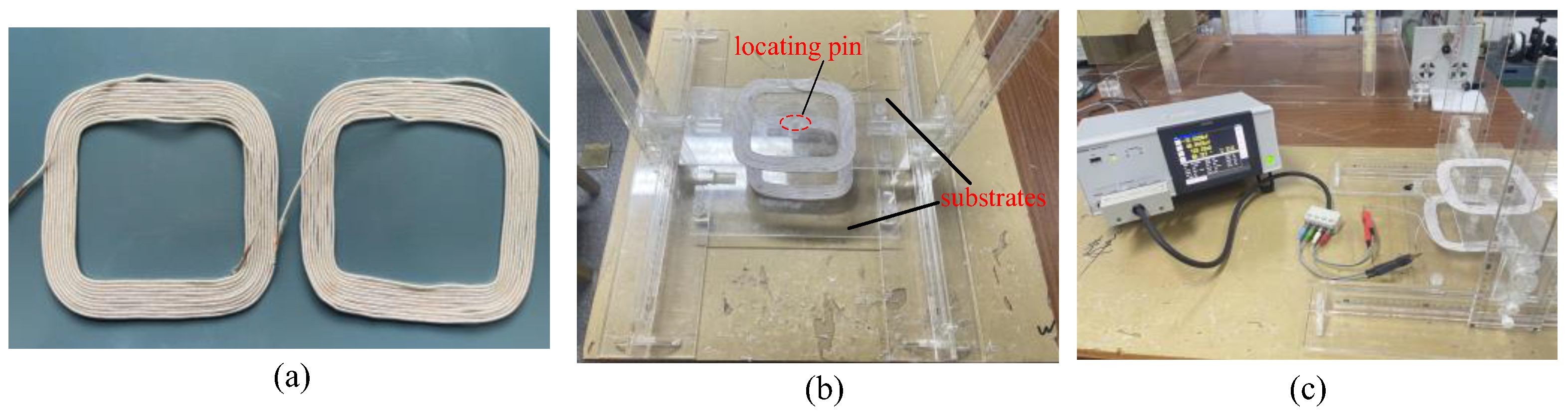
4. Experimentation and Numerical Simulation
4.1. Mutual Inductance Measurement Experiment
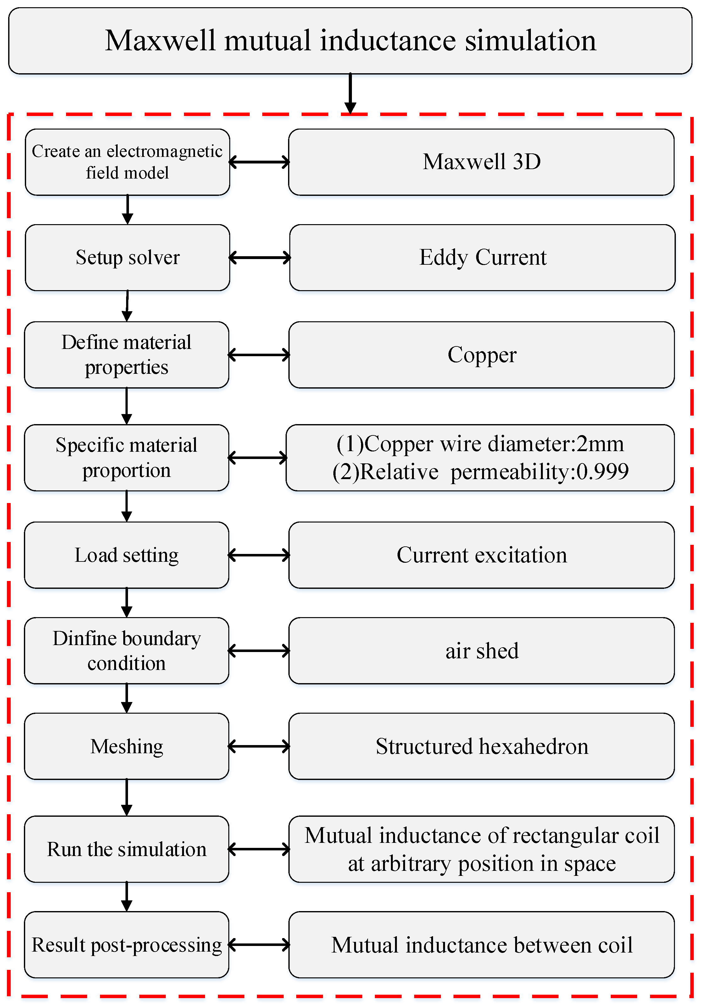
4.2. Numerical Simulation of Mutual Inductance
5. Results and Discussion
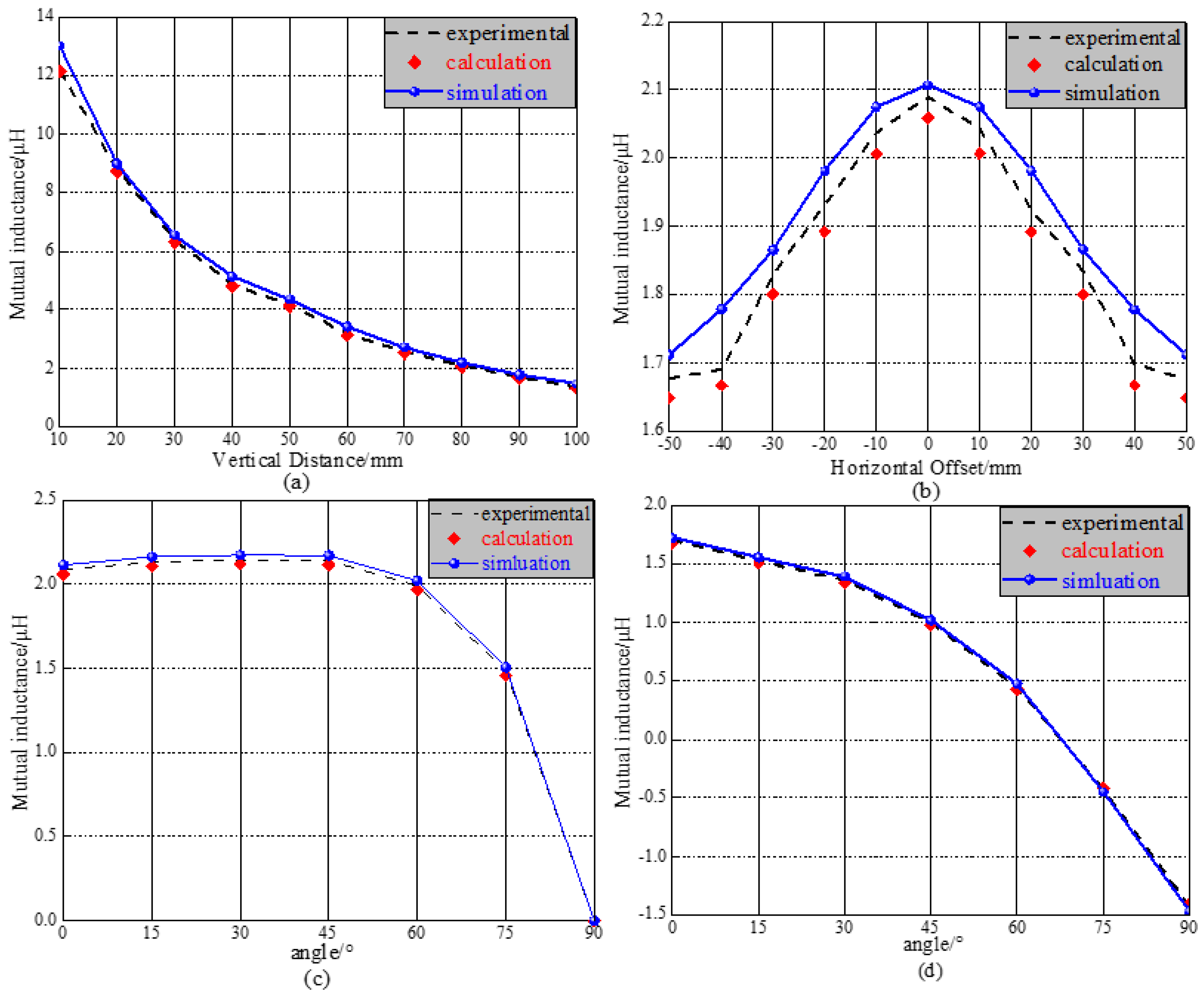
5.1. Comparison of Calculation and Experimental Results
- (1)
- Influence of vertical offset on mutual inductance
- (2)
- Influence of horizontal offset on mutual inductance
- (3)
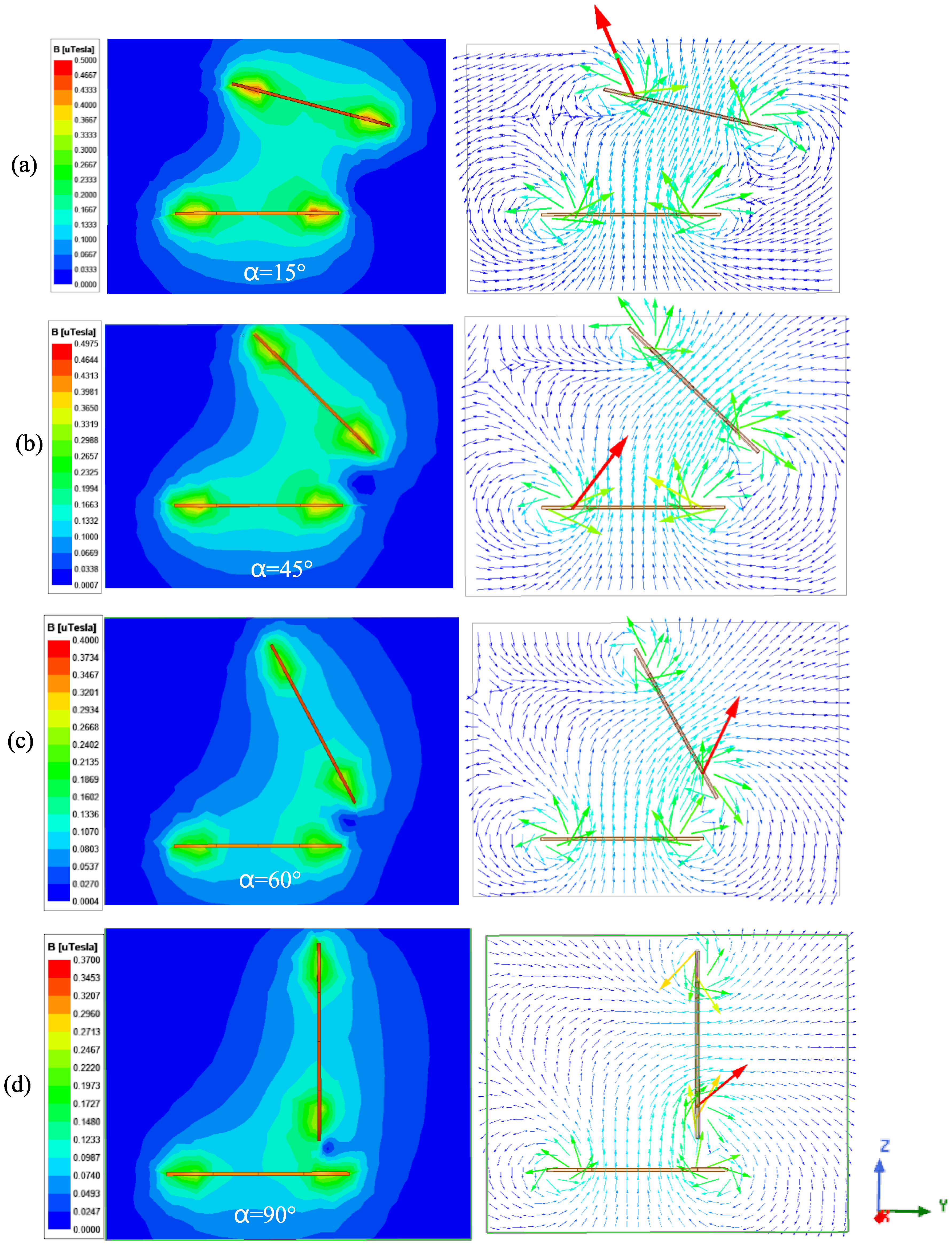
- Influence of angular rotation on mutual inductance
- (4)
- Influence of angular rotation with offset on mutual inductance
5.2. Comparison of Calculation with Experimental and Simulation Results
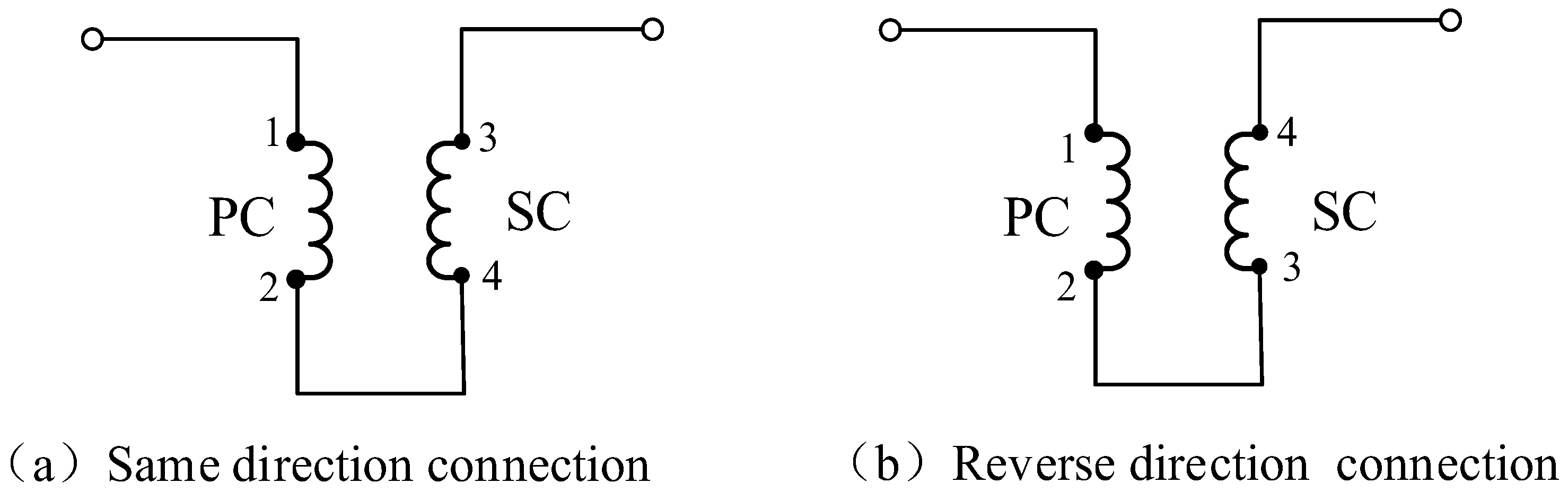
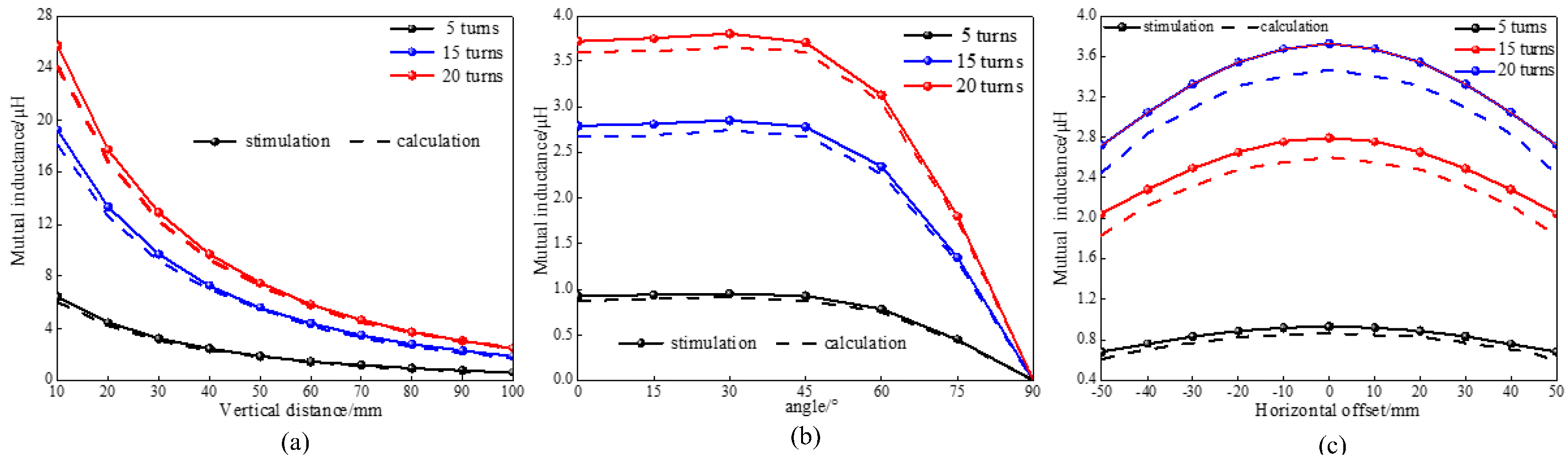
5.3. Mutual Inductance Verification Between Coils with Different Turns
6. Conclusions
Author Contributions
Funding
Institutional Review Board Statement
Informed Consent Statement
Data Availability Statement
Acknowledgments
Conflicts of Interest
References
- Poletkin, K.V. Calculation of magnetic force and torque between two arbitrarily oriented circular filaments using Kalantarov–Zeitlin’s method. Int. J. Mech. Sci. 2022, 220, 107159. [Google Scholar] [CrossRef]
- Yi, J.; Yang, P.; Li, Z.; Kong, P.; Li, J. Mutual inductance calculation of circular coils for an arbitrary position with a finite magnetic core in wireless power transfer systems. IEEE Trans. Transp. Electrif. 2022, 9, 1950–1959. [Google Scholar] [CrossRef]
- Narukullapati, B.K.; Bhattacharya, T.K. Determination of a stable lateral region of a floating disc–mathematical analysis and FEM simulation. Alex. Eng. J. 2021, 60, 3107–3118. [Google Scholar] [CrossRef]
- Aydin, E.; Yildiriz, E.; Aydemir, M.T. A new semi-analytical approach for self and mutual inductance calculation of hexagonal spiral coil used in wireless power transfer systems. Electr. Eng. 2021, 103, 1769–1778. [Google Scholar] [CrossRef]
- Spengler, N.; While, P.T.; Meissner, M.V.; Wallrabe, U.; Korvink, J.G. Magnetic Lenz lenses improve the limit-of-detection in nuclear magnetic resonance. PLoS ONE 2017, 128, e0182779. [Google Scholar] [CrossRef]
- Schweighart, S.A. Electromagnetic Formation Flight Dipolesolution Planning; Massachusetts Institute of Technology: Cambridge, MA, USA, 2005. [Google Scholar]
- Li, Y.; Chen, J.; Liu, Y.; Zhao, X.; Fu, M.; He, Z. An Accurate Modeling and Suppression Method for Current Imbalance in Dual-Receiver WPT Systems for Low-voltage and High-current Applications. IEEE Trans. Transp. Electrif. 2023, 10, 7065–7075. [Google Scholar] [CrossRef]
- Inamori, T.; Sugawara, Y.; Satou, Y. Electromagnetic panel deployment and retraction using the geomagnetic field in LEO satellite missions. Adv. Space Res. 2015, 56, 2455–2472. [Google Scholar] [CrossRef]
- Inamori, T.; Satou, Y.; Sugawara, Y.; Ohsaki, H. Electromagnetic panel deployment and retraction in satellite missions. Acta Astronaut. 2015, 109, 14–24. [Google Scholar] [CrossRef]
- Hu, W.; He, Q.; Sun, X.; Yang, Y.; Yang, B. Design of an innovative active hinge for Self-deploying/folding and vibration control of solar panels. Sens. Actuators A Phys. 2018, 281, 196–208. [Google Scholar] [CrossRef]
- Zhu, Y.; Cai, W.; Yang, L.; Huang, H. Flatness-based trajectory planning for electromagnetic spacecraft proximity operations in elliptical orbits. Acta Astronaut. 2018, 152, 342–351. [Google Scholar] [CrossRef]
- Wu, D.; Huang, C.; Yang, F.; Sun, Q. Analytical calculations of self-and mutual inductances for rectangular coils with lateral misalignment in IPT. IET Power Electron. 2019, 12, 4054–4062. [Google Scholar]
- Babic, S.; Akyel, C. Improvement in calculation of the self-and mutual inductance of thin-wall solenoids and disk coils. IEEE Trans. Magn. 2000, 36, 1970–1975. [Google Scholar] [CrossRef]
- Lyu, Y.-L.; Meng, F.-Y.; Yang, G.-H.; Che, B.-J.; Wu, Q.; Sun, L.; Erni, D.; Li, J.L.-W. A method of using nonidentical resonant coils for frequency splitting elimination in wireless power transfer. IEEE Trans. Power Electron. 2015, 30, 6097–6107. [Google Scholar] [CrossRef]
- Conway, J.T. Inductance calculations for noncoaxial coils using bessel functions. IEEE Trans. Magn. 2007, 43, 1023–1034. [Google Scholar] [CrossRef]
- Smeets, J.P.C.; TOverboom, T.; Jansen, J.W.; Lomonova, E.A. Inductance calculation nearby conducting material. IEEE Trans. Magn. 2014, 50, 1–4. [Google Scholar] [CrossRef]
- Hussain, I.; Woo, D.K. Simplified mutual inductance calculation of planar spiral coil for wireless power applications. Sensors 2022, 22, 1537. [Google Scholar] [CrossRef]
- Maxwell, J.C. A Treatise on Electricity and Magnetism, 3rd ed.; Dover Publications Inc.: Garden City, NY, USA, 1954; Volume 2. [Google Scholar]
- Babic, S.; Sirois, F.; Akyel, C.; Girardi, C. Mutual inductance calculation between circular filaments arbitrarily positioned in space: Alternative to Grover’s formula. IEEE Trans. Magn. 2010, 46, 3591–3600. [Google Scholar] [CrossRef]
- Grover, F.W. Inductance Calculations: Working Formulas and Tables; Courier Corporation: North Chelmsford, MA, USA, 2004. [Google Scholar]
- Poletkin, K.V.; Korvink, J.G. Efficient calculation of the mutual inductance of arbitrarily oriented circular filaments via a generalisation of the Kalantarov-Zeitlin method. J. Magn. Magn. Mater. 2019, 483, 10–20. [Google Scholar] [CrossRef]
- Gao, S.; Wang, Q.; Li, G.; Qian, Z.; Ye, Q.; Lu, Z.; Li, Z. Spherical actuator attitude measurement method based on multi-to-one WPT modeling. Measurement 2022, 197, 111346. [Google Scholar] [CrossRef]
- Qiao, X.; Wu, Y.; Chen, M.; Niu, Y. Modeling and optimization of the magnetically coupled resonant wireless power transfer used in rotary ultrasonic machining process. Sens. Actuators A Phys. 2023, 354, 114290. [Google Scholar] [CrossRef]
- Li, H.; Li, J.; Wang, K.; Chen, W.; Yang, X. A maximum efficiency point tracking control scheme for wireless power transfer systems using magnetic resonant coupling. IEEE Trans. Power Electron. 2014, 30, 3998–4008. [Google Scholar] [CrossRef]
- Chen, N.; Liu, L.J.; Qie, D.S.; Zhou, H.; Li, B.; Li, Y.; Zhang, H. Design and Electromagnetic Analysis of Induction Coil of Cold Crucible by ANSYS. He-Huaxue Yu Fangshe Huaxue J. Nucl. Radiochem. 2014, 36, 21–26. [Google Scholar]
- Ji, Y.; Wang, H.; Lin, J.; Guan, S.; Feng, X.; Li, S. The mutual inductance calculation between circular and quadrilateral coils at arbitrary attitudes using a rotation matrix for airborne transient electromagnetic systems. J. Appl. Geophys. 2014, 111, 211–219. [Google Scholar] [CrossRef]
- Durmus, F.; Karagol, S. Mutual Inductance Calculation for Planar Square and Hexagonal Coils. Arab. J. Sci. Eng. 2022, 47, 3409–3420. [Google Scholar] [CrossRef]
- Tavakkoli, H.; Abbaspour-Sani, E.; Khalilzadegan, A.; Rezazadeh, G.; Khoei, A. Analytical study of mutual inductance of hexagonal and octagonal spiral planer coils. Sens. Actuators A Phys. 2016, 247, 53–64. [Google Scholar] [CrossRef]
- Song, M.; Zhou, D.; Yu, P.; Zhao, Y.; Wang, Y.; Tan, Y.; Li, J. Analytical calculation and experimental verification of superconducting electrodynamic suspension system using null-flux ground coil. IEEE Trans. Intell. Transp. Syst. 2021, 23, 14978–14989. [Google Scholar] [CrossRef]
- Cheng, Y.H.; Shu, Y.M. A new analytical calculation of the mutual inductance of the coaxial spiral rectangular coils. IEEE Trans. Magn. 2013, 50, 1–6. [Google Scholar] [CrossRef]
- He, J.L.; Rote, D.M.; Chen, S.S. Characteristics and Computer Model Simulation of Magnetic Damping Forces in Maglev Systems; ANL/ESD/TM-66; Argonne National Lab: Argonne, IL, USA, 1994. [Google Scholar]
- Joy, E.R.; Dalal, A.; Kumar, P. Accurate computation of mutual inductance of two air core square coils with lateral and angular misalignments in a flat planar surface. IEEE Trans. Magn. 2013, 50, 1–9. [Google Scholar] [CrossRef]
- Li, J. Research on Calculation Method of Mutual Inductance Between Rectangular Coils in Wireless Power Transfer Systems. Master’s Thesis, Hunan University of Technology, Zhuzhou, China, 2023. [Google Scholar]


| Symbols | Meanings | Symbols | Meanings |
|---|---|---|---|
| α, β, γ | Euler angles | Mt | Mutual inductance of a multi-turn coil |
| Rαβγ | Coordinate transformation matrix | dρ, dτ | Radius and tangent of projected circular plane |
| B | Magnetic induction intensity | dl, l1, l2 | Primary coil side length |
| A | Vector magnetic potential | dl’, l’1, l’2 | Side length of secondary coil |
| ψ | Magnetic linkage | a, b | Side length of primary coil of example model |
| M | Mutual inductance | c, d | Side length of secondary coil of example model |
| N1 | Turns of the primary coil | h | Vertical height |
| N2 | Turns of the secondary coil | Δy | Horizontal displacement |
| Vertical Distance h/cm | M/μH (Magnetic Flux Density) | M/μH (Neumann Formula) | M/Μh (This Work’s Equation (31)) |
|---|---|---|---|
| 2 | 18.05 | 18.08 | 18.10 |
| 3 | 13.97 | 14.00 | 14.10 |
| 4 | 11.16 | 11.18 | 11.26 |
| 5 | 9.11 | 9.14 | 9.20 |
| 6 | 7.54 | 7.57 | 7.64 |
| 7 | 6.32 | 6.35 | 6.42 |
| 8 | 5.34 | 5.38 | 5.43 |
| 9 | 4.46 | 4.50 | 4.56 |
| 10 | 3.83 | 3.86 | 3.90 |
| Horizontal Distance Δy/mm | M/μH (Magnetic Flux Density) | M/μH (Neumann Formula) | M/μH (This Work’s Equation (31)) |
|---|---|---|---|
| 1 | 17.04 | 17.08 | 17.10 |
| 2 | 15.76 | 15.79 | 15.82 |
| 3 | 14.24 | 14.28 | 14.30 |
| 4 | 12.75 | 12.79 | 12.80 |
| 5 | 11.35 | 11.38 | 11.40 |
| 6 | 10.04 | 10.09 | 10.11 |
| 7 | 8.88 | 8.92 | 8.94 |
| 8 | 7.61 | 7.64 | 7.66 |
| 9 | 6.75 | 6.77 | 6.79 |
| 10 | 5.27 | 5.30 | 5.32 |
| Horizontal Distance Δy/mm | M/μH (Magnetic Flux Density) | M/μH (Neumann Formula) | M/μH (This Work’s Equation (31)) |
|---|---|---|---|
| 10 | 2.7281 | 2.7369 | 2.7587 |
| 20 | 2.6498 | 2.6793 | 2.6891 |
| 30 | 2.5244 | 2.5413 | 2.5510 |
| 40 | 2.3586 | 2.3719 | 2.3767 |
| 50 | 2.1606 | 2.1724 | 2.1883 |
| 60 | 1.9395 | 1.9577 | 1.9675 |
| 70 | 1.7045 | 1.7233 | 1.7531 |
| 80 | 1.4646 | 1.4769 | 1.4868 |
| 90 | 1.2279 | 1.2413 | 1.2482 |
| Deflection Angle α/° | M/μH (Magnetic Flux Density) | M/μH (Neumann Formula) | M/μH (This Work’s Equation (31)) |
|---|---|---|---|
| 0 | 2.7535 | 2.7591 | 2.7691 |
| 10 | 2.7301 | 2.7687 | 2.7787 |
| 20 | 2.7705 | 2.7735 | 2.7935 |
| 30 | 2.8181 | 2.8241 | 2.8341 |
| 40 | 2.8141 | 2.8232 | 2.8385 |
| 50 | 2.6765 | 2.6741 | 2.6971 |
| 60 | 2.323 | 2.3259 | 2.3459 |
| 70 | 1.7119 | 1.721 | 1.731 |
| 80 | 0.8948 | 0.9012 | 0.9111 |
| 90 | 0 | 0 | 0 |
| α/rad | β/rad | γ/rad | M/μH (Neumann Formula) | M/μH (This Work’s Equation (28)) |
|---|---|---|---|---|
| π/3 | 0 | π/6 | 12.66 | 12.476 |
| π/4 | π/3 | π/3 | 14.64 | 14.519 |
| π/3 | π/4 | π/2 | 15.70 | 15.505 |
| π/4 | π/5 | 2π/3 | 23.92 | 23.417 |
| π/5 | π/6 | 5π/6 | 26.16 | 25.935 |
| Coil Parameters | Size | Material Quality |
|---|---|---|
| Length of the innermost circle/mm | 100 | copper wire |
| Innermost ring width/mm | 80 | |
| Turns of the primary coil | 10 | |
| Turns of the secondary coil | 10 | |
| Diameter/mm | 2 |
| No. | Vertical Distance h/mm | Me/μh | Mc/μh | εe/% |
|---|---|---|---|---|
| 1 | 10 | 12.1632 | 12.0112 | 1.25 |
| 2 | 20 | 8.7757 | 8.6539 | 1.39 |
| 3 | 30 | 6.3631 | 6.2723 | 1.43 |
| 4 | 40 | 4.8511 | 4.7783 | 1.50 |
| 5 | 50 | 4.1551 | 4.100 | 1.33 |
| 6 | 60 | 3.1863 | 3.126 | 1.89 |
| 7 | 70 | 2.5664 | 2.5193 | 2.15 |
| 8 | 80 | 2.0895 | 2.0591 | 1.46 |
| 9 | 90 | 1.7034 | 1.6718 | 1.86 |
| 10 | 100 | 1.3559 | 1.3355 | 1.51 |
| No. | Horizontal Offset Δy/mm | Me/μh | Mc/μh | εe/% |
|---|---|---|---|---|
| 11 | −50 | 1.6777 | 1.6490 | 1.71 |
| 12 | −40 | 1.6905 | 1.6677 | 1.35 |
| 13 | −30 | 1.8300 | 1.8008 | 1.6 |
| 14 | −20 | 1.9309 | 1.8916 | 2.04 |
| 15 | −10 | 2.0366 | 2.0067 | 1.47 |
| 16 | 0 | 2.0895 | 2.0591 | 1.45 |
| 17 | 10 | 2.0426 | 2.0067 | 1.77 |
| 18 | 20 | 1.9243 | 1.8916 | 1.76 |
| 19 | 30 | 1.8346 | 1.8008 | 1.84 |
| 20 | 40 | 1.6993 | 1.6677 | 1.86 |
| 21 | 50 | 1.6993 | 1.6490 | 1.58 |
| No. | α/° | Me/μh | Mc/μh | εe/% |
|---|---|---|---|---|
| 22 | 0 | 2.0895 | 2.0591 | 1.46 |
| 23 | 15 | 2.1293 | 2.1079 | 1.01 |
| 24 | 30 | 2.1465 | 2.1196 | 1.25 |
| 25 | 45 | 2.1400 | 2.1142 | 1.20 |
| 26 | 60 | 1.9903 | 1.965 | 1.27 |
| 27 | 75 | 1.4824 | 1.4596 | 1.54 |
| 28 | 90 | 0.00095 | 0 | / |
| No. | Secondary Coil Center Coordinates (0,40,80)/mm | |||
|---|---|---|---|---|
| α/° | Me/μh | Mc/μh | εe/% | |
| 29 | 0 | 1.6993 | 1.6677 | 1.86 |
| 30 | 15 | 1.5223 | 1.5015 | 1.37 |
| 31 | 30 | 1.3564 | 1.3301 | 1.2 |
| 32 | 45 | 0.9949 | 0.9719 | 1.31 |
| 33 | 60 | 0.44 | 0.4234 | 1.5 |
| 34 | 75 | −0.4225 | −0.4169 | 1.33 |
| 35 | 90 | −1.4244 | −1.3991 | 1.77 |
Disclaimer/Publisher’s Note: The statements, opinions and data contained in all publications are solely those of the individual author(s) and contributor(s) and not of MDPI and/or the editor(s). MDPI and/or the editor(s) disclaim responsibility for any injury to people or property resulting from any ideas, methods, instructions or products referred to in the content. |
© 2025 by the authors. Licensee MDPI, Basel, Switzerland. This article is an open access article distributed under the terms and conditions of the Creative Commons Attribution (CC BY) license (https://creativecommons.org/licenses/by/4.0/).
Share and Cite
Chen, J.; Yao, G.; Wang, M.; Zhou, L.; Gao, K.; Zhou, P.; Liu, R. An Effective Method for Calculation of Mutual Inductance Between Rectangular Coils at Arbitrary Positions in Space. Sensors 2025, 25, 3265. https://doi.org/10.3390/s25113265
Chen J, Yao G, Wang M, Zhou L, Gao K, Zhou P, Liu R. An Effective Method for Calculation of Mutual Inductance Between Rectangular Coils at Arbitrary Positions in Space. Sensors. 2025; 25(11):3265. https://doi.org/10.3390/s25113265
Chicago/Turabian StyleChen, Junlin, Guofeng Yao, Min Wang, Liming Zhou, Kuiyang Gao, Peilei Zhou, and Ruiyao Liu. 2025. "An Effective Method for Calculation of Mutual Inductance Between Rectangular Coils at Arbitrary Positions in Space" Sensors 25, no. 11: 3265. https://doi.org/10.3390/s25113265
APA StyleChen, J., Yao, G., Wang, M., Zhou, L., Gao, K., Zhou, P., & Liu, R. (2025). An Effective Method for Calculation of Mutual Inductance Between Rectangular Coils at Arbitrary Positions in Space. Sensors, 25(11), 3265. https://doi.org/10.3390/s25113265