Communication

Multiple-Cumulant-Matrices-Based Method for Exact NF Polarization Localization with COLD Array

1
Faculty of Electrical Engineering and Computer Science, Ningbo University, Ningbo 315211, China
2
School of Materials Science and Chemical Engineering, Ningbo University, Ningbo 315211, China
*
Author to whom correspondence should be addressed.
These authors contributed equally to this work.
Sensors 2025, 25(10), 3244; https://doi.org/10.3390/s25103244
Submission received: 11 April 2025 / Revised: 14 May 2025 / Accepted: 20 May 2025 / Published: 21 May 2025

Abstract

:
As a key technology for the fifth-generation of mobile communications, massive MIMO systems enable massive user access via large-scale arrays. However, their dense deployment extends the near-field (NF) region, introducing new localization complexities. Based on an exact spherical wavefront model, this paper proposes a multiple-cumulant-matrices-based method for NF source localization using a Co-centered Orthogonal Loop and Dipole (COLD) array. Firstly, following the physical numbering of array elements, we can construct multiple polarization cumulant matrices, which can then be cascaded into a long matrix. Next, the signal subspace can be obtained through eigen-decomposition of this long matrix, from which the horizontal and vertical components can be further separated. By applying ESPRIT, joint angle, range, and polarization parameters can be estimated. In addition, the asymptotic variances for joint spatial and polarization parameters are analyzed. Compared with existing NF polarization algorithms, the proposed method exhibits better parameter estimation and is consistent with a theoretical asymptotic performance.

1. Introduction

In array signal processing, source localization is an important problem, with widespread applications in wireless communication and radar systems [1,2,3,4,5,6,7]. In practical scenarios, such as multiple-input multiple-output (MIMO) systems equipped with a large antenna array, the target source crosses the Fresnel boundary, entering the NF region. When the sources move from the far-field (FF) region, the planar wavefront assumption is not available, requiring characterization by a spherical wavefront that is bivariate in both the Direction-of-Arrival (DOA) and range parameters, and the propagation attenuation induces range-dependent amplitude variations among sensors, thereby rendering FF localization methods ineffective.
Nowadays, numerous algorithms for FF localization have been successfully generalized for NF applications, such as the maximum-likelihood (ML) method [8], second-order statistics (SOS) methods [9,10,11,12] and fourth-order cumulant (FOC) methods [13,14,15]. Based on the wavefront approximation principle, i.e., Fresnel approximation, these methods suffer from amplitude and phase loss compared with practical wireless environments [16,17,18]. For amplitude attenuation, several works have addressed this issue. In [19], a delay-correlation SOS-based method was proposed considering amplitude attenuation; however, to satisfy the symmetric property of the array, this method utilizes an approximation phase item. Recently, based on an exact spherical wavefront model, Ref. [20] proposed a delay FOC-based method, which can achieve underdetermined estimation by using a cumulant matrix and vectorization operation, but it requires 3-D spectral search, suffering from an extremely high complexity. In [21], a mixed FF and NF localization method was proposed using coarse and fine estimation from the amplitude and phase item, and this method is closed-from, but suffers from aperture loss.
Although all the abovementioned algorithms were designed for effective spatial parameter estimation, they neglect polarization information, which is a fundamental feature of electromagnetic sources. With the introduction of polarization-sensitive arrays, both spatial and polarization parameter localization are possible. In [22], a generalized ESPRIT method was performed for NF polarization source localization based on a cross-dipole array, which can decouple spatial and polarization parameters, but it can only estimate spatial parameters. In [23], a rank-reduction-based method was proposed, but it still required a 2-D spectral search to estimate polarization parameters. The aforementioned methods [8,9,10,11,13,15,22,23] employed Fresnel approximation. Then, a COLD array-based exact NF polarization localization method was proposed in [24], which can estimate the polarization rotational matrix, but estimates spatial parameters from range-dependent amplitude attenuation, resulting in a lower estimation accuracy.
To address the issue of exact NF polarization source localization, by employing a COLD array, this paper proposes a multiple-cumulant-based DOA estimation method. Cumulant matrices related to various array elements are calculated, which can then be combined in a long matrix, avoiding the aperture loss. By using ESPRIT, the proposed method can achieve spatial and polarization decoupling and joint estimation of four-dimensional (4-D) parameters. Moreover, joint spatial and polarization parameter performance evaluation was performed to demonstrate the algorithm’s validity.This paper represents an original contribution in three aspects:
(1) Unlike conventional NF polarization localization methods, the proposed algorithm completely avoids systematic errors induced by model approximations.
(2) Multiple cumulant matrices are constructed and cascaded into a long matrix, so the manifold matrix for joint parameters can be estimated without aperture loss.
(3) We derive an analytical expression for the asymptotic variance under an exact NF polarization condition.

2. Signal Model

As depicted in Figure 1, assume that there is a linear array deployed along the x-axis consisting of 2 L + 1 COLD antennas, where the center antenna, i.e., the 0-th antenna, serves as amplitude-phase reference. Consider K narrowband completely polarized signals impinging on the array from θ 1 , r 1 , , θ k , r k , θ K , r K with corresponding polarization parameters γ 1 , η 1 , , γ k , η k , , γ K , η K , where θ k , r k , γ k and η k represent the angle, range, polarization angle, and polarization phase difference of the k-th signal s k t , respectively.
Based on spherical wavefront geometry, the range between the k-th source and l-th sensor is given by
r l , k = r k 2 + d l 2 2 r k d l sin θ k ,
where d l represents the distance between the l-th COLD and reference point, l = L , . . . , 0 , . . . , L . Therefore, the exact spatial amplitude-phase corresponding to between k-th source and l-th sensor be expressed as
b l , k = r k r l , k e j 2 π λ r k r l , k = ρ l , k e j τ l , k ,
where ρ l , k stands for the amplitude attenuation, τ l , k = 2 π λ r k r l , k stands for the exact phase shift caused by propagation delay, and then we can obtain the spatial steering vector of the k-th source, which can be expressed as
b θ k , r k = b L , k , . . . , b 0 , k , . . . , b L , k T .
Additionally, for the COLD array, the polarization steering vector of the k-th source can be written as
g γ k , η k = sin γ k e j η k cos γ k .
Hence, we can obtain a spatial and polarization joint steering vector as
a θ k , r k , γ k , η k = g γ k , η k b θ k , r k ,
where ⊗ represents the Kronecker product, a θ k , r k , γ k , η k is the 2 2 L + 1 × 1 vector. At time t, the signal data vector of the COLD array can be expressed as the following 2 2 L + 1 × 1 vector:
x t = k = 1 K g γ k , η k b θ k , r k s k t + n t = G B s t + n t = As t + n t ,
where ⊙ represents the Khatri–Rao product, A = a θ 1 , r 1 , γ 1 , η 1 , . . . , a θ K , r K , γ K , η K signifies the 2 2 L + 1 × K manifold matrix, B = b θ 1 , r 1 , . . . , b θ K , r K stands for spatial manifold matrix, G = g γ 1 , η 1 , . . . , g γ K , η K stands for the 2 × K polarization manifold matrix, s t = s 1 t , . . . , s K t T represents the K × 1 signal vector, and n t represents the 2 2 L + 1 × 1 additive noise vector of COLD array with zero mean.
From (5), the signal data vector can be divided into horizontal and vertical components, expressed as
x t = x 1 t x 2 t = BP 1 BP 2 s t + n t ,
where x 1 t is composed of the first 2 L + 1 rows of x t , x 1 t = x 1 , L t , . . . , x 1 , L t T , and x 2 t containing the last 2 L + 1 rows, x 2 t = x 2 , L t , . . . , x 2 , L t T . P 1 and P 2 are diagonal matrices, whose k-th diagonal elements are sin γ k e j η k and cos γ k , respectively. Hence, the steering vector a θ k , r k , γ k , η k can be rewritten as two components, i.e., a θ k , r k , γ k , η k = a 1 , L , k , . . . , a 1 , L , k , a 2 , L , k , . . . , a 2 , L , k T , where a 1 , l , k = sin γ k e j η k b l , k and a 2 , l , k = cos γ k b l , k .

3. The Proposed Method

According to the definition in [25], the FOC of x p t , x q t , x i t , x j t is given by
C x p , x q * , x i , x j * = E { x p x q * x i x j * } E { x p x q * } E { x i x j * } E { x p x i } E { x q * x j * } E { x p x j * } E { x q * x i } .

3.1. Spatial Manifold Matrix Estimation

Using the signal data vector, we can construct the FOC matrix of the l-th COLD antenna C l as follows [26]
C l = i = 1 2 cum x i , l t , x i , 0 * t , x t , x H t = i = 1 2 k = 1 K a i , l , k a i , 0 , k a k a k H × cum s k t , s k * t , s k t , s k * t = k = 1 K b l , k a k a k H c 4 s k ,
where · * represents complex conjugate, · H represents conjugate transpose, and the FOC matrix C l can be expressed in compact form as C l = A Φ l C 4 s A H with dimensions of 2 2 L + 1 × 2 2 L + 1 , c 4 s k = cum s k t , s k * t , s k t , s k * t stands for the FOC of k-th signal, Φ l is diagonal matrix, whose diagonal elements are related to the amplitude-phase corresponding of l-th COLD array, Φ l = diag ρ l , 1 e j τ l , 1 , . . . , ρ l , K e j τ l , K , C 4 s = diag c 4 s 1 , . . . , c 4 s K .
From (9), for the complete COLD array, we can construct 2 L + 1 similar cumulant matrices by varying the sensor index. Subsequently, a long matrix Ξ can be obtained by cascading these cumulant matrices
Ξ = C L C 0 C L = A Φ L C 4 s A H A Φ 0 C 4 s A H A Φ L C 4 s A H ,
where Φ 0 is the identity matrix. The covariance matrix of this joint long matrix is given by
R = E { Ξ Ξ H } .
The eigen-decomposition of the covariance matrix R yields
R = U Σ U H = U S Σ S U S H + U N Σ N U N H ,
where U contains the eigenvectors of R , Σ is the diagonal matrix, the signal subspace U S corresponds to the K largest eigenvalues with the dimensions 2 2 L + 1 2 × K , while the noise subspace U N corresponds to the 2 2 L + 1 2 K smallest eigenvalues.
The signal subspace U S comprises the subspace associated with the cumulant matrices of all array elements, which can be partitioned into 2 L + 1 block sub-matrices as follows:
U S = U S L T , , U S 0 T , , U S L T T ,
where U S 0 , formed by the elements from rows 2 2 L + 1 L + 1 to 2 2 L + 1 L + 1 of U S , represents the subspace corresponding to the cumulant matrix of the reference. Due to the rotation-invariant property between the reference cumulant matrix and other sensors’ matrices, there exists a full-rank matrix T satisfying
U S = A Φ L A Φ 0 A Φ L T .
From (14), between U S l and U S 0 , we can have the following relationship as
U S l = U S 0 T 1 Φ l T = U S 0 Ψ l ,
where Ψ l = T 1 Φ l T , Φ l is diagonal matrix, whose diagonal elements are the eigenvalues of Ψ l . Using the least squares (LS), we can obtain the following formulation:
min Δ U 2 s . t . U S l + Δ U = U S 0 Ψ l .
From (16), we can derive
Ψ l = U S 0 H U S 0 1 U S 0 H U S l = U S 0 + U S l ,
where · + represents pseudo-inverse. Obviously, Φ ^ l can be estimated by performing the eigen-decomposition of Ψ l . Iterate through different array elements and repeat the aforementioned steps (17), the spatial manifold matrix B ^ can be estimated as follows:
B ^ = diag 1 Φ ^ L diag 1 Φ ^ 0 diag 1 Φ ^ L = b ^ θ 1 , r 1 , . . . , b ^ θ K , r K ,
where diag 1 · represents the row vector operation, and the estimation of spatial steering vector of k-th signal is b ^ θ k , r k = b ^ L , k , . . . , b ^ 0 , k , . . . , b ^ L , k T .

3.2. Polarization Parameters Estimation

From (7), obviously, the FOC matrix C l can be divided into
C l = B Φ l P 1 C 4 s B H B Φ l P 2 C 4 s B H ,
where the first half of C l corresponds to the horizontal component, while the second half corresponds to the vertical component. Therefore, U S l can be further divided into
U S l = U S l , 1 T , U S l , 2 T T ,
where U S l , 1 is formed by the first 2 L + 1 rows of U S l and U S l , 2 formed by the last 2 L + 1 rows. Sub-matrices U S L , 1 , . . . , U S L , 1 and U S L , 2 , . . . , U S L , 2 can be extracted from the signal subspace U S , the horizontal and vertical component subspaces, E h and E v , can then be constructed as
E h = U S L , 1 U S 0 , 1 U S L , 1 , E v = U S L , 2 U S 0 , 2 U S L , 2 .
By applying ESPRIT, we can rewrite (21) as
E h = B Φ L P 1 B Φ L P 1 T , E v = B Φ L P 2 B Φ L P 2 T .
With component matrices E h and E v , we can obtain the following matrix:
D = E h + E v = T 1 P 1 1 P 2 T = T 1 PT .
Substituting matrices P 1 and P 2 into (23), the polarized diagonal matrix P can be expressed as
P = diag cot γ 1 e j η 1 , . . . , cot γ K e j η K .
Like (15), P ^ can be estimated by performing eigen-decomposition of D . As a result, the polarization parameters estimates of k-th source are given by
γ ^ k = arc cot P ^ k η ^ k = angle P ^ k ,
where P ^ k represents the k-th diagonal element of P ^ .

3.3. Coarse Estimation

The angle ( · ) operator can extract the phase of b ^ l , k but introduces phase ambiguity when the spacing between two COLDs exceeds λ / 2 . To resolve this ambiguity, disambiguation operations utilizing the coarse reference estimates are employed to obtain the unambiguous phase τ ^ l , k for fine estimation. Then, we impose structural constraints on the array configuration to obtain unambiguous reference values. Assuming there exist three sensors, whose positions are d p , d c , and d q , respectively, the phase factor will be coarse but unambiguous, when the spacing of these three sensors satisfies d p d c λ / 2 and d q d c λ / 2 . The relationship between these sensors can be established as
r k 2 + d c 2 2 r k d c sin α k r k 2 + d p 2 2 r k d p sin α k = ψ ^ c , p , k 2 π / λ r k 2 + d c 2 2 r k d c sin α k r k 2 + d q 2 2 r k d q sin α k = ψ ^ c , q , k 2 π / λ ,
where ψ ^ c , p , k = angle B ^ p , k / B ^ c , k and ψ ^ c , p , k = angle B ^ q , k / B ^ c , k . In this work, d c represents the coordinates of the reference element, while d p = d 1 and d q = d 1 denote the coordinates of its adjacent elements located at λ / 2 on either side. Hence, from (18), the unambiguous phases of the k-th steering vector can be denoted as τ ^ 1 , k and τ ^ 1 , k . Then, the coarse estimates of θ k and r k can be given by
r ^ k c = d 1 τ ^ 1 , k 2 π / λ 2 d 1 τ ^ 1 , k 2 π / λ 2 + d 1 d 1 2 d 1 d 1 2 2 d 1 τ ^ 1 , k 2 π / λ 2 d 1 τ ^ 1 , k 2 π / λ θ ^ k c = arc sin 2 r ^ k c τ ^ 1 , k 2 π / λ τ ^ 1 , k 2 π / λ 2 + d 1 2 2 r ^ k c d 1 .

3.4. Fine Estimation

Let ϕ ^ l , k denote the ambiguous phase. According to the (2), there exists an integer-multiplicity set S l relationship between ϕ ^ l , k and τ ^ l , k , expressed as S l = ϕ ^ l , k + 2 π n n Z . With (27), by using θ ^ k c and r ^ k c , we can construct the unambiguous phase reference values as follows:
τ ^ l , k c o = 2 π λ r ^ k c r ^ l , k c .
Thus, the exact estimation τ ^ l , k is the value in S l that minimizes the deviation from the coarse estimate τ ^ l , k c o , i.e.,
τ ^ l , k = arg min n τ l , k c o ϕ ^ l , k + 2 π n .
Furthermore, the phase term satisfies the following relationship with respect to the angle and range:
τ l , k 2 π / λ = r k r l , k = r k r k 2 + d l 2 2 r k d l sin θ k .
Substituting the τ ^ L , k , , τ ^ l , k , , τ ^ L , k into (30) and simplifying, we can construct coefficient matrices which consist of 2 L equation relations
V k = 2 τ ^ L , k 2 π / λ 2 d L 2 τ ^ L , k 2 π / λ 2 d L , W k = τ ^ L , k 2 π / λ 2 d L 2 τ ^ L , k 2 π / λ 2 d L 2 ,
where the unknown vector to be solved is denoted as Δ f , k T = r k r k sin θ k T . These vectors can be further rewritten as a matrix equation V k × Δ f , k = W k . By applying LS, the Δ ^ f , k can be solved as
Δ ^ f , k = V k H V k 1 V k H W k = V k + W k .
Finally, the fine estimates of angle and range can be derived as
r ^ k f i = Δ ^ f , k 1 θ ^ k f i = arc sin Δ ^ f , k 2 Δ ^ f , k 1 .

3.5. Asymptotic Variance for Joint Parameters

The theoretical phase at the l-th sensor from the k-th source is given by
ϑ l , k = e j 2 π λ r k r k 2 + d l 2 2 r k d l sin θ k ,
while the corresponding polarization factor for the k-th source is
p k = cot γ k e j η k .
Additionally, the estimate ϑ ^ l , k of ϑ l , k , is the l , k -th element of B ^ , while p ^ k is obtained from the k-th diagonal element of P ^ . Thus, the deviations between the true and estimated values are δ ϑ l , k = ϑ ^ l , k ϑ l , k and δ p k = p ^ k p k [13].
For simplicity, the fine estimates of angle and range are defined as θ ^ k and r ^ k , whose deviations are defined as δ θ k = θ ^ k θ k and δ r k = r ^ k r k . In addition, the deviations of polarization angle and polarization phase difference are defined as δ γ k = γ ^ k γ k and δ η k = η ^ k η k , respectively.
Using the first-order Taylor expansion for ϑ l , k and p k , we can obtain
ϑ l , k ϑ ^ l , k + θ k θ ^ k ϑ l , k θ k + r k r ^ k ϑ l , k r k ,
p k p ^ k + γ k γ ^ k p k γ k + η k η ^ k p k η k ,
where the partial derivatives of ϑ l , k to θ ^ k and r ^ k are
ϑ l , k θ k = ϑ l , k j 2 π λ r k d l cos θ k r k 2 + d l 2 2 r k d l sin θ k , ϑ l , k r k = ϑ l , k j 2 π λ 1 2 r k 2 d l sin θ k 2 r k 2 + d l 2 2 r k d l sin θ k ,
and
p k γ k = 1 sin 2 γ k e j η k , p k η k = j cot γ k e j η k .
Substituting (38) and (39) into (36) and (37), respectively, the final expansion yields
j 2 π r k d l λ r l , k cos θ k ϑ l , k δ θ k + j 2 π r l , k r k + d l sin θ k λ r l , k ϑ l , k δ r k = δ ϑ l , k ,
1 sin 2 γ k e j η k δ γ k j cot γ k e j η k δ η k = δ p k .
With the same principle as (31), 2 L equations can be listed, which can than be rewritten in matrix form
Z k = j υ L , k ϑ L , k j ω L , k ϑ L , k j υ L , k ϑ L , k j ω L , k ϑ L , k , Λ k = δ ϑ L , k δ ϑ L , k ,
where
υ l , k = 2 π r k d l λ r l , k cos θ k , ω l , k = 2 π r l , k r k + d l sin θ k λ r l , k ,
and the unknown vector to be solved is Γ k = δ θ k δ r k T , which satisfies Z k × Γ k = Λ k . By applying LS, we have the following results:
Γ k = Z k H Z k 1 Z k H Λ k = Z k + Λ k ,
Thus, the closed-form variance expressions can be given by
E δ θ k 2 = E Z k + Λ k Z k + Λ k T 1 , E δ r k 2 = E Z k + Λ k Z k + Λ k T 2 .
where · 1 represents the first diagonal element, and · 2 represents the second diagonal element.
According to (41), δ γ k and δ η k correspond to the real and imaginary parts of δ p k , respectively. By exploiting the conjugate symmetry, the closed-form expressions for δ γ k and δ η k are
δ γ k = δ p k e j η k + δ p k * e j η k sin 2 γ k 2 , δ η k = δ p k e j η k δ p k * e j η k 2 j cot γ k ,
and the variances of δ γ k and δ η k can be given by
E δ γ k 2 = E δ p k e j η k + δ p k * e j η k 2 sin 4 γ k 4 E δ η k 2 = E δ p k e j η k δ p k * e j η k 2 4 cot 2 γ k .
The steps of the proposed method are summarized in Table 1.

3.6. Computational Complexity

In this section, we analyze the computational complexity of the proposed method, focusing on (a) 2 L + 1 FOC matrix construction requires O 4 2 L + 1 × 2 L + 1 2 N flops; (b) the complexity of computing the covariance matrix R requires O { 8 2 L + 1 5 } ; (c) the eigen-decomposition of the covariance matrix requires O { 8 2 L + 1 6 } multiplication operations; (d) the complexity of manifold matrix estimation requires O { 4 2 L + 1 K 2 + 2 K 2 } ; (e) the complexity in computing D is O { 2 2 L + 1 K 2 } . Overall, the proposed method is approximately O { 4 2 L + 1 3 N + 8 2 L + 1 5 + 8 2 L + 1 6 + 12 L + 8 K 2 } . The computational complexity of the proposed algorithm and that of other comparative methods are summarized in Table 2, where n θ , n r , n γ , n η represent the number of searches for DOA, range, polarization angle, and polarization phase difference. As shown in Table 2, the proposed method showed better efficiency than FR-RARE and G-ESPRIT without peak search, though requiring more operations than He’s method.

3.7. CRB Derivation

This section derives the closed-form deterministic Cramér–Rao Bound (CRB) expressions for jointly estimating the DOA, range, and polarization parameters under exact near-field polarization conditions. We define the real-valued vector ε = θ T r T η T γ T T , where θ = θ 1 , θ 2 , , θ K T , r = r 1 , r 2 , , r K T , η = η 1 , η 2 , , η K T and γ = γ 1 , γ 2 , , γ K T . Thus, the CRB for the parameters in ε is given by [24]
CRB ε = σ n 2 2 N Υ H P Θ Υ 1 4 1 4 T R s T 1 .
where Υ = Υ θ , Υ r , Υ γ , Υ η , Υ θ = Θ θ 1 , , Θ θ K , Υ r = Θ r 1 , , Θ r K , Υ γ = Θ γ 1 , , Θ γ K , Υ η = Θ η 1 , , Θ η K , P Θ = I 2 2 L + 1 Θ Θ H Θ 1 Θ H .

4. Simulation Results

Simulation experiments were performed to evaluate the performance of the proposed method compared with the existing G-ESPRIT method [22], FR-RARE method [23], He’s method [24], and the CRB [24] for an exact NF polarization scenario.

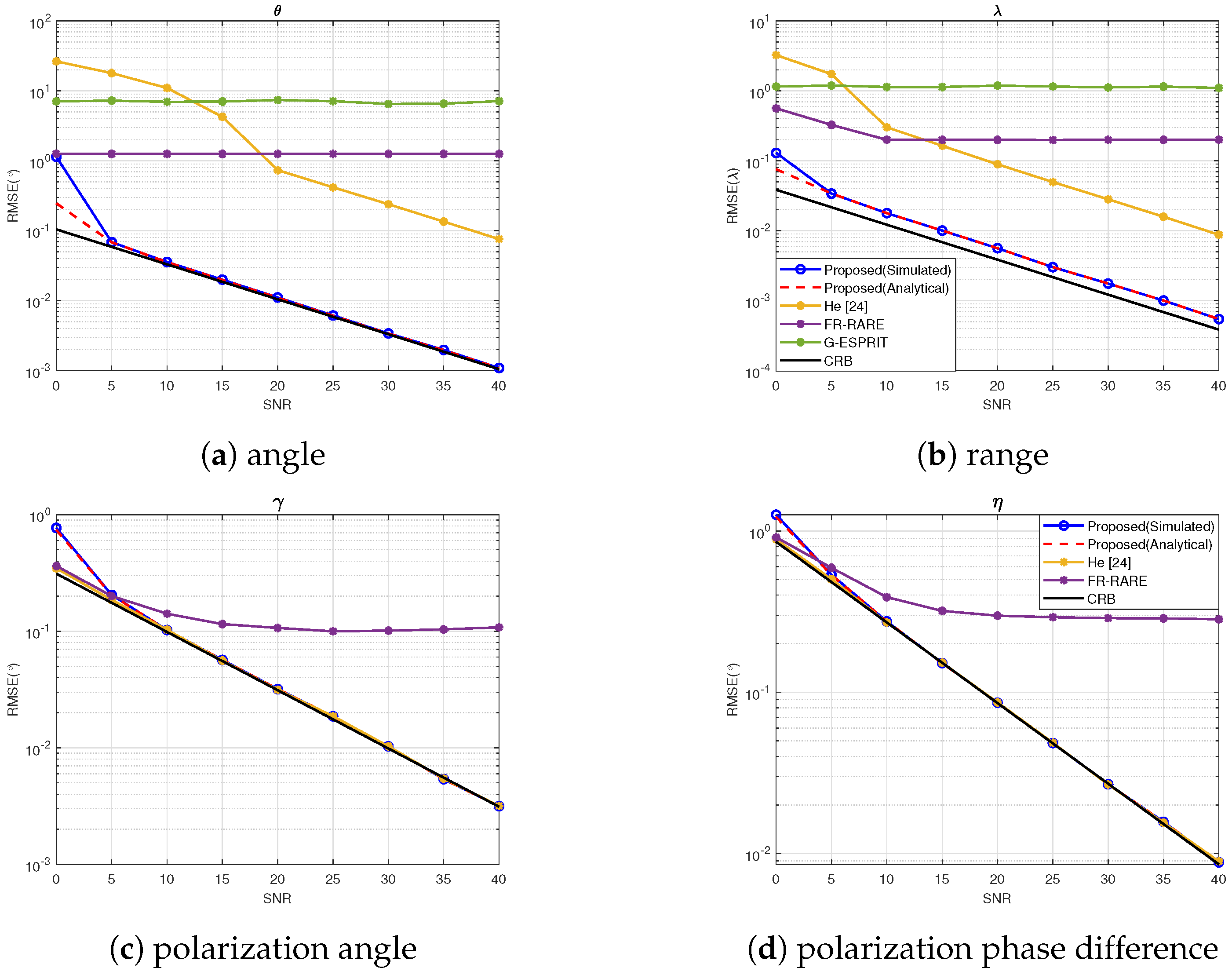
4.1. Experiment 1: RMSE vs. SNR

In this section, a symmetric linear COLD array consisting of 9 antenna elements was considered, with uniform spacing λ / 4 . Two uncorrelated NF sources arrived at the COLD array, with parameters 15 , 5.5 λ , 20 , 20 and 20 , 6 λ , 30 , 40 and the number of snapshots was set to N = 2000 . The root-mean-square error (RMSE) was utilized to evaluate the performance, defined as
RMSE = 1 500 K k = 1 K i = 1 500 x k x ^ i , k 2 ,
where x k stands for the true value of parameters θ k , r k , γ k , η k and x ^ i , k represents the estimate of the θ ^ i , k , r ^ i , k , γ ^ i , k , η ^ i , k at the i-th run in 500 Monte-Carlo trials.
Figure 2 shows the RMSE curves of the spatial and polarization parameters, when the SNR varied from 0 dB to 40 dB. It can be seen that the estimation performance of both the proposed algorithm and He’s method improved as the SNR increased. As an amplitude-attenuation based method, He’s method exhibited limited estimation accuracy, suffering from mismatch under the low SNR. Among all the algorithms, the proposed algorithm more closely approximated the CRB and could exploit the whole aperture. In addition, due to the model approximation, G-ESPRIT and FR-RARE showed performance “saturation”.

4.2. Experiment 2: Scatter for Spatial and Polarization

In this section, we derived the maximum number of identifiable NF sources. Based on an analysis of the rank of the manifold matrix, the theoretical limit was established when the matrix satisfied the full-rank condition. Consider a 9-element COLD array with antenna positions 2 , 1.6 , 1.1 , 0.5 , 0 , 0.5 , 1.3 , 1.5 , 2.2 . Assume that 8 uncorrelated NF sources arrive at the array with locations 15 , 5.5 λ , 20 , 20 , 5 , 6 λ , 30 , 40 , 5 , 6.5 λ , 45 , 30 , 20 , 7.5 λ , 50 , 25 , 25 , 5.8 λ , 25 , 10 , 30 , 6 λ , 20 , 42 , 35 , 6.3 λ , 40 , 10 , and 40 , 6.8 λ , 30 , 50 . With the SNR fixed at 25 dB and the number of snapshots be 2000, Figure 3 presents scatter plots of joint parameters in a 2-D plane based on 500 Monte Carlo runs. As shown in Figure 3, the 4-D parameters were all closely distributed near the true values, which were automatically paired.

4.3. Experiment 3: RMSE vs. Path Loss Exponent

In this section, we tested the algorithm performance with difference path loss exponents. The location of the sources and other parameters were set the same as in Experiment 1, and the path loss exponent varied from 2 to 6. As shown in Figure 4, the RMSE was approximately constant with the exponential increase in path loss. The reasons for the performance saturation of He’s method, G-ESPRIT, and FR-RARE were the same as in Experiment 1.

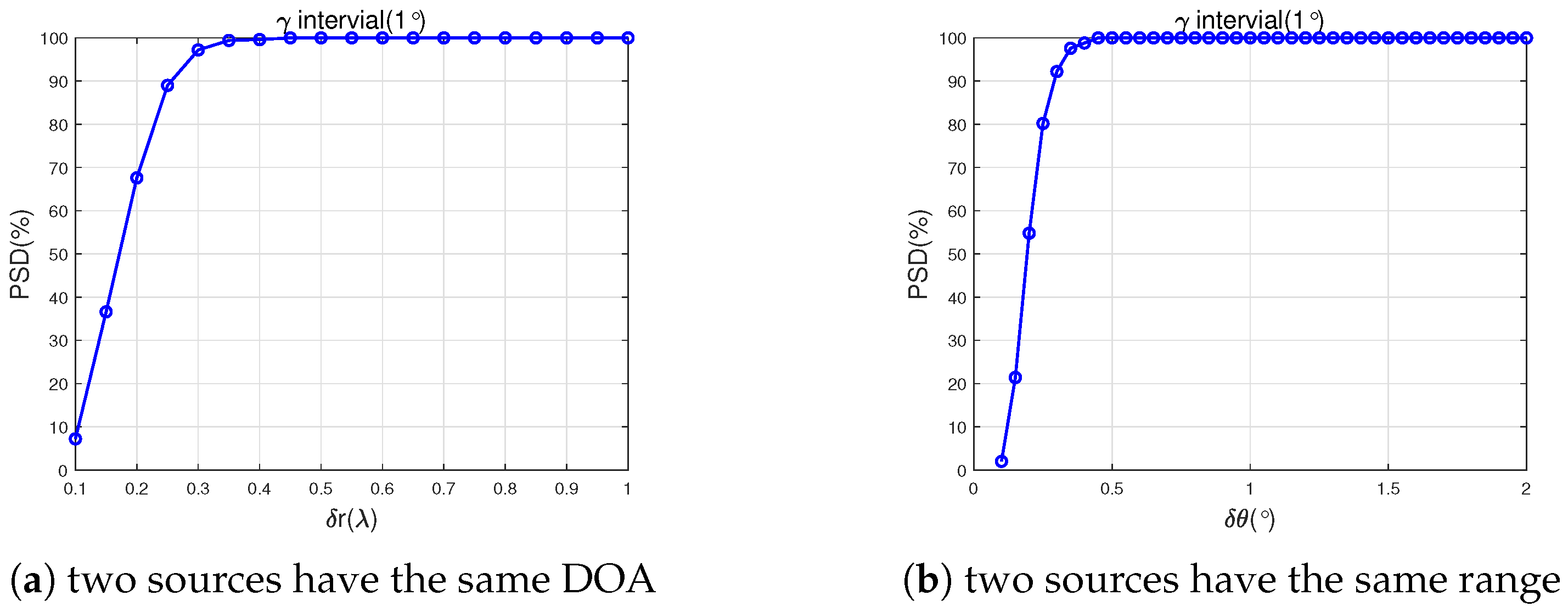
4.4. Experiment 4: Detection Capability for Closely Spaced Targets

In this section, we considered a scenario where two closely spaced impinging signals had the same DOA or same range. In Figure 5a, two sources had the same DOA parameterized by 20 , 5.5 λ , 20 , 20 , and 20 , 5.5 λ + δ λ , 30 , 40 , in Figure 5b, the two sources had the same range parameterized by 20 , 5.5 λ , 20 , 20 , and 20 + δ θ , 5.5 λ , 30 , 40 , and the other parameters were set as same as Experiment 2. Successful detection was defined as a polarization angle RSME between the estimated γ ^ and true value γ less than 1 . The probability of successful detection (PSD) was defined as a successful detection trial under 500 Monte-Carlo runs. As shown in Figure 5, when the DOA interval was larger than 0 . 5 or the range interval was larger than 0.4 λ , the proposed method offered 100 % PSD for polarization angle; that is, we could refer to polarization information to distinguish two closely spaced impinging signals.

4.5. Experiment 5: RMSE vs. Correlation Coefficient

Assume that there are two correlated sources parameterized by 10 , 5.5 λ , 15 , 45 and 22 , 5.8 λ , 35 , 90 , the other parameters were set the same as in Experiment 2, where correlation coefficient varied from 0.1 to 0.9. As can be seen from Figure 6, the RMSE of all spatial and polarization parameters increased with the increase in the correlation coefficient.

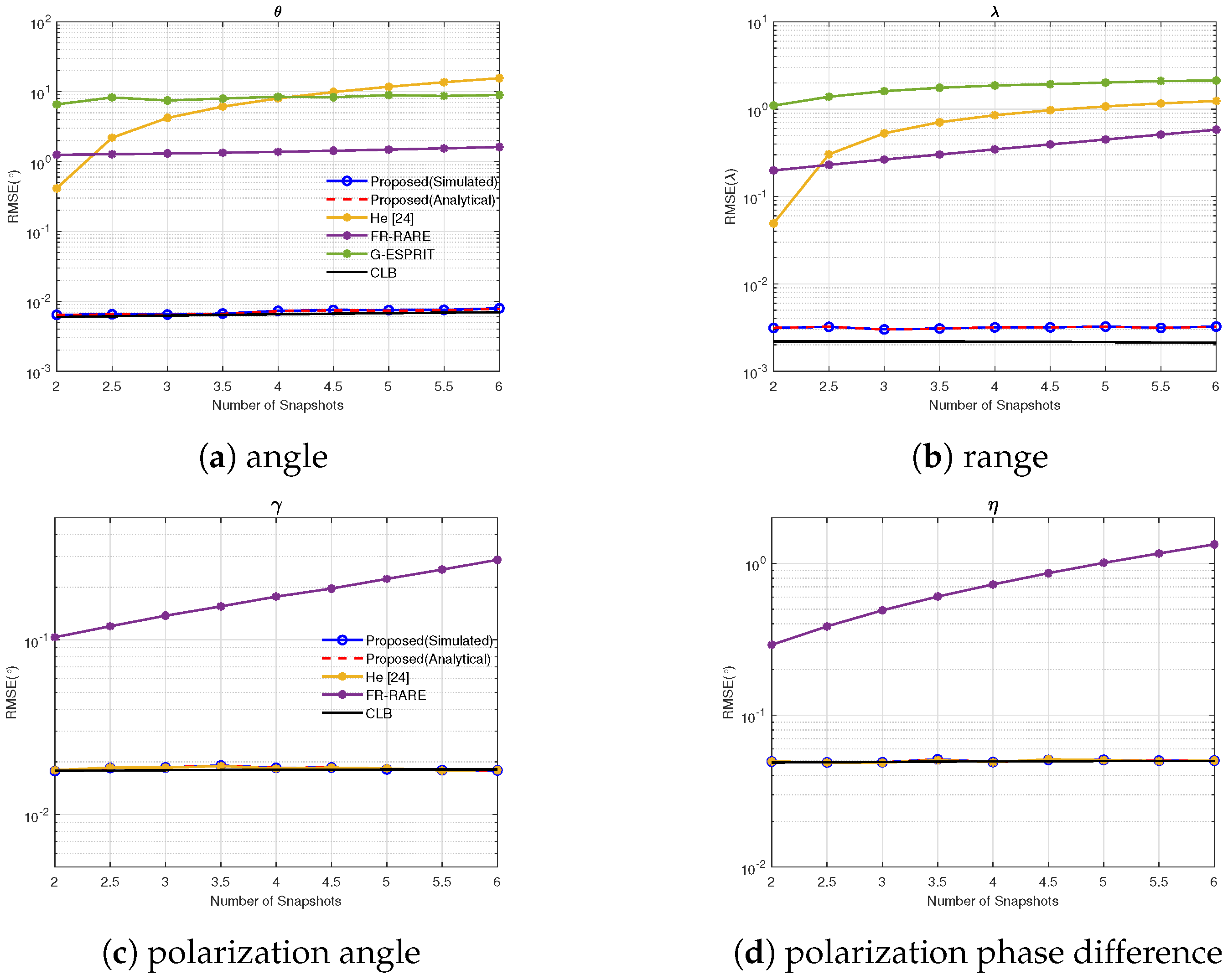
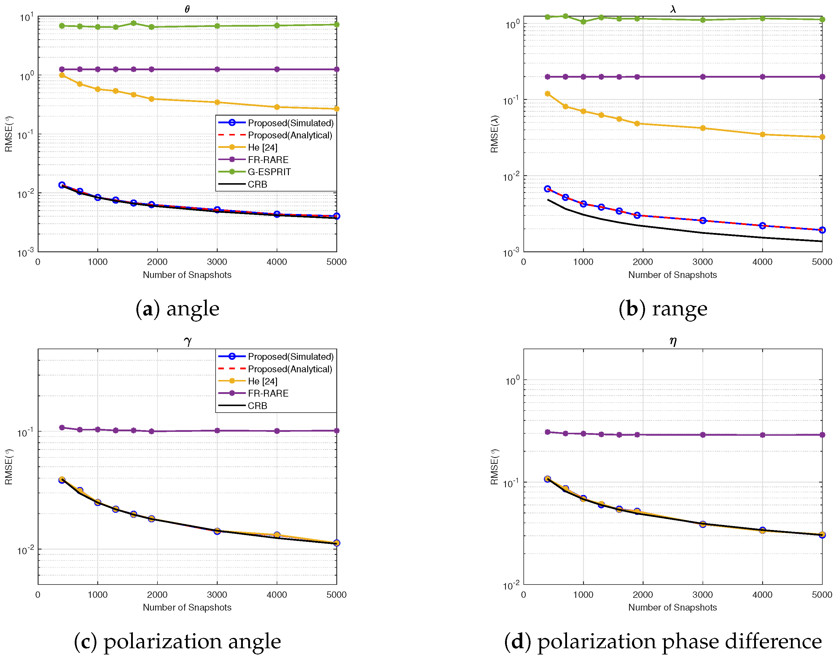
4.6. Experiment 6: RMSE vs. Snapshots

In this experiment, we evaluated the performance by varying the number of snapshots from 400 to 5000, the SNR was fixed as 25 dB, with the same source parameters as in Experiment 1. The RMSE of the 4-D parameters vs. the number of snapshots is shown in Figure 7. The results demonstrate that the RMSE of both the proposed algorithm and He’s method decreased with increasing snapshots, while our method had a better performance. In contrast, G-ESPRIT and FR-RARE were always in a performance saturation state.

5. Conclusions

The primary contribution of this paper is source localization under an exact NF polarization scenario. With a COLD array, a multiple-cumulant-matrices-based method was proposed for joint 4-D parameter estimation, formulated via least squares principles, with neither approximation nor aperture loss. After that, the asymptotic variances of 4-D parameters were derived. Simulation results demonstrated that the algorithm had superior performance under the exact NF polarization scenario.

Author Contributions

Conceptualization, J.Z.; methodology, J.Z., H.M. and Z.L.; software, J.Z. and Z.L.; validation, J.Z. and Z.L.; formal analysis, J.Z. and H.W.; investigation, J.Z. and Z.L.; resources, W.L.; data curation, J.Z. and H.M.; writing—original draft preparation, J.Z. and H.C.; writing—review and editing, H.C. and W.L.; visualization, H.C.; supervision, H.C.; project administration, H.C.; funding acquisition, H.C. and W.L. All authors have read and agreed to the published version of the manuscript.

Funding

This research was supported by Zhejiang Provincial Natural Science Foundation of China under Grant No. LY23F010003, and by the “Pioneer” and “Leading Goose” R & D Program of Zhejiang Province under Grant 2024C01105, and by the National Natural Science Foundation of China under Grant 62001256.

Institutional Review Board Statement

Not applicable.

Informed Consent Statement

Not applicable.

Data Availability Statement

The data used to support the findings of this study are available from the corresponding author upon request.

Acknowledgments

We sincerely thank all the reviewers for their patient reviews of and valuable suggestions for this article.

Conflicts of Interest

We declare that we have no financial and personal relationships with other people or organizations that can inappropriately influence our work, there is no professional or other personal interests of any nature or kind in any product, service, and/or company that could be construed as influencing the position presented in, or the review of, the manuscript entitled.

References

  1. Sakhnini, A.; De Bast, S.; Guenach, M.; Bourdoux, A.; Sahli, H.; Pollin, S. Near-Field Coherent Radar Sensing Using a Massive MIMO Communication Testbed. IEEE Trans. Wirel. Commun. 2022, 21, 6256–6270. [Google Scholar] [CrossRef]
  2. Ali, E.; Balfaqih, M.; Shglouf, I.; Alrayes, M.; Balfagih, Z. Two-Dimensional DOA Zero-Forcing Precoding for Enhanced Spectral Efficiency in Cell-Free Massive MIMO. In Proceedings of the 2025 22nd International Learning and Technology Conference, Jeddah, Saudi Arabia, 15–16 January 2025; Volume 22, pp. 164–169. [Google Scholar] [CrossRef]
  3. Chen, H.; Fang, J.; Wang, W.; Liu, W.; Tian, Y.; Wang, Q.; Wang, G. Near-Field Target Localization for EMVS-MIMO Radar with Arbitrary Configuration. IEEE Trans. Aerosp. Electron. Syst. 2024, 60, 5406–5417. [Google Scholar] [CrossRef]
  4. Weißer, F.; Utschick, W. DoA-Aided Channel Estimation for One-Bit Quantized Systems. In Proceedings of the 2025 14th International ITG Conference on Systems, Communications and Coding (SCC), Karlsruhe, Germany, 10–13 March 2025; pp. 1–6. [Google Scholar] [CrossRef]
  5. Elbir, A.M.; Celik, A.; Eltawil, A.M. NEAT-MUSIC: Auto-Calibration of DOA Estimation for Terahertz-Band Massive MIMO Systems. IEEE Wirel. Commun. Lett. 2024, 13, 451–455. [Google Scholar] [CrossRef]
  6. Buzzi, S.; Grossi, E.; Lops, M.; Venturino, L. Foundations of MIMO Radar Detection Aided by Reconfigurable Intelligent Surfaces. IEEE Trans. Signal Process. 2022, 70, 1749–1763. [Google Scholar] [CrossRef]
  7. Chen, H.; Yi, Z.; Jiang, Z.; Liu, W.; Tian, Y.; Wang, Q.; Wang, G. Spatial-Temporal-Based Underdetermined Near-Field 3-D Localization Employing a Nonuniform Cross Array. IEEE J. Sel. Top. Signal Process. 2024, 18, 561–571. [Google Scholar] [CrossRef]
  8. Chen, J.; Hudson, R.; Yao, K. Maximum-likelihood source localization and unknown sensor location estimation for wideband signals in the near-field. IEEE Trans. Signal Process. 2002, 50, 1843–1854. [Google Scholar] [CrossRef]
  9. Gao, F.; Gershman, A. A generalized ESPRIT approach to direction-of-arrival estimation. IEEE Signal Process. Lett. 2005, 12, 254–257. [Google Scholar] [CrossRef]
  10. Huang, Y.D.; Barkat, M. Near-field multiple source localization by passive sensor array. IEEE Trans. Antennas Propag. 1991, 39, 968–975. [Google Scholar] [CrossRef]
  11. He, J.; Swamy, M.N.S.; Ahmad, M.O. Efficient Application of MUSIC Algorithm Under the Coexistence of Far-Field and Near-Field Sources. IEEE Trans. Signal Process. 2012, 60, 2066–2070. [Google Scholar] [CrossRef]
  12. Zaman, F.; Akbar, S.; Akhtar, Z.; Phanomchoeng, G. Efficient Technique for Joint Parameter Estimation of Mixed Far Field Targets and Near Field Jammers in Phased Array Radar. IEEE Access 2025, 13, 55887–55898. [Google Scholar] [CrossRef]
  13. Yuen, N.; Friedlander, B. Performance analysis of higher order ESPRIT for localization of near-field sources. IEEE Trans. Signal Process. 1998, 46, 709–719. [Google Scholar] [CrossRef]
  14. Molaei, A.M.; del Hougne, P.; Fusco, V.; Yurduseven, O. Efficient Joint Estimation of DOA, Range and Reflectivity in Near-Field by Using Mixed-Order Statistics and a Symmetric MIMO Array. IEEE Trans. Veh. Technol. 2022, 71, 2824–2842. [Google Scholar] [CrossRef]
  15. Liang, J.; Liu, D. Passive Localization of Mixed Near-Field and Far-Field Sources Using Two-stage MUSIC Algorithm. IEEE Trans. Signal Process. 2010, 58, 108–120. [Google Scholar] [CrossRef]
  16. Friedlander, B. Localization of Signals in the Near-Field of an Antenna Array. IEEE Trans. Signal Process. 2019, 67, 3885–3893. [Google Scholar] [CrossRef]
  17. Fang, J.; Chen, H.; Liu, W.; Yang, S.; Yuen, C.; So, H.C. Three-Dimensional Localization of Mixed Near-Field and Far-Field Sources Based on a Unified Exact Propagation Model. IEEE Trans. Signal Process. 2025, 73, 245–258. [Google Scholar] [CrossRef]
  18. He, J.; Li, L.; Shu, T.; Truong, T.K. Mixed Near-Field and Far-Field Source Localization Based on Exact Spatial Propagation Geometry. IEEE Trans. Veh. Technol. 2021, 70, 3540–3551. [Google Scholar] [CrossRef]
  19. Jiang, Z.; Chen, H.; Liu, W.; Wang, G. 3-D temporal-spatial-based near-field source localization considering amplitude attenuation. Signal Process. 2022, 201, 108735. [Google Scholar] [CrossRef]
  20. Jin, L.; Chen, H.; Fang, J.; Liu, W.; Tian, Y.; Wang, G. Fourth-Order Cumulant Based 3-D Near-Field Underdetermined Parameter Estimation With Exact Spatial Propagation Model. In Proceedings of the ICASSP 2025—2025 IEEE International Conference on Acoustics, Speech and Signal Processing (ICASSP), Hyderabad, India, 6–11 April 2025; pp. 1–5. [Google Scholar] [CrossRef]
  21. He, J.; Shu, T.; Li, L.; Truong, T.K. Mixed Near-Field and Far-Field Localization and Array Calibration With Partly Calibrated Arrays. IEEE Trans. Signal Process. 2022, 70, 2105–2118. [Google Scholar] [CrossRef]
  22. He, J.; Ahmad, M.O.; Swamy, M.N.S. Near-Field Localization of Partially Polarized Sources with a Cross-Dipole Array. IEEE Trans. Aerosp. Electron. Syst. 2013, 49, 857–870. [Google Scholar] [CrossRef]
  23. Tao, J.W.; Liu, L.; Lin, Z.Y. Joint DOA, Range, and Polarization Estimation in the Fresnel Region. IEEE Trans. Aerosp. Electron. Syst. 2011, 47, 2657–2672. [Google Scholar] [CrossRef]
  24. He, J.; Li, L.; Shu, T. Near-Field Parameter Estimation for Polarized Source Using Spatial Amplitude Ratio. IEEE Commun. Lett. 2020, 24, 1961–1965. [Google Scholar] [CrossRef]
  25. Mendel, J. Tutorial on higher-order statistics (spectra) in signal processing and system theory: Theoretical results and some applications. Proc. IEEE 1991, 79, 278–305. [Google Scholar] [CrossRef]
  26. Ma, H.; Tao, H.; Xie, J.; Cheng, X. Parameters Estimation of 3-D Near-Field Sources with Arbitrarily Spaced Electromagnetic Vector-Sensors. IEEE Commun. Lett. 2022, 26, 2764–2768. [Google Scholar] [CrossRef]
Figure 1. COLD array configuration for exact NF source localization.
Sensors 25 03244 g001
Figure 2. RMSE vs. SNR.
Sensors 25 03244 g002
Figure 3. Scatter plots of 4-D parameters estimation.
Sensors 25 03244 g003
Figure 4. RMSE vs. path loss exponent.
Sensors 25 03244 g004
Figure 5. PSD vs. parameter interval.
Sensors 25 03244 g005
Figure 6. RMSE vs. correlation coefficient.
Sensors 25 03244 g006
Figure 7. RMSE vs. the number of snapshots.
Sensors 25 03244 g007
Table 1. Algorithmic steps.
StepOperation
1Construct C L , , C 0 , , C L via (9) and the long matrix Ξ
can be obtain via (10).
2Compute the covariance matrix R and perform eigen-decomposition
to obtain signal subspace U S .
3Using the LS and eigen-decomposition, we can obtain
Φ ^ L , , Φ ^ 0 , , Φ ^ L to construct B ^ .
4Extract U S L , 1 , , U S L , 1 and U S L , 2 , , U S L , 2 from U S to construct E h and E v .
Matrix P is obtained by performing eigen-decomposition on matrix D ,
where matrix D can be obtain from (33). From the diagonal element of P ,
we have the estimates γ ^ 1 , , γ ^ k , , γ ^ K and η ^ 1 , , η ^ k , , η ^ K .
5for  k 1 , K  do
   (1) The closed-form coarse estimation r ^ k c and θ ^ k c can be obtained via (26) and (27).
   (2) Via (28) and (29), we can disambiguate the phase to construct matrices
       V k and W k .
   (3) Based on LS method, the fine estimation r ^ k f i and θ ^ k f i can be obtained by
      solving (33).
End for
Table 2. Computational complexity of all compared algorithms.
MethodComplexity
Proposed O { 4 2 L + 1 3 N + 8 2 L + 1 5 + 8 2 L + 1 6 + 12 L + 8 K 2 }
FR-RARE [22] O { 4 2 L + 1 2 N + 8 2 L + 1 3 + 4 L + 1 4 L + 2 K 2 L + 1 K n θ
+ 2 L + 1 32 L + 16 4 K + 8 K n r + 2 2 L + 1 4 L + 2 K n γ n η }
G-ESPRIT [23] O { 4 2 L + 1 2 N + 8 2 L + 1 3 + 32 L K 2 n θ + 4 2 L + 1 4 L + 2 K n r }
He [24] O { 4 2 L + 1 2 N + 8 2 L + 1 3 + 4 2 L + 1 2 K + 2 2 L + 1 K 2 }
Disclaimer/Publisher’s Note: The statements, opinions and data contained in all publications are solely those of the individual author(s) and contributor(s) and not of MDPI and/or the editor(s). MDPI and/or the editor(s) disclaim responsibility for any injury to people or property resulting from any ideas, methods, instructions or products referred to in the content.

