

Performance Comparison of Multipixel Biaxial Scanning Direct Time-of-Flight Light Detection and Ranging Systems With and Without Imaging Optics

Abstract

1. Introduction
2. Materials and Methods
2.1. Rate Model
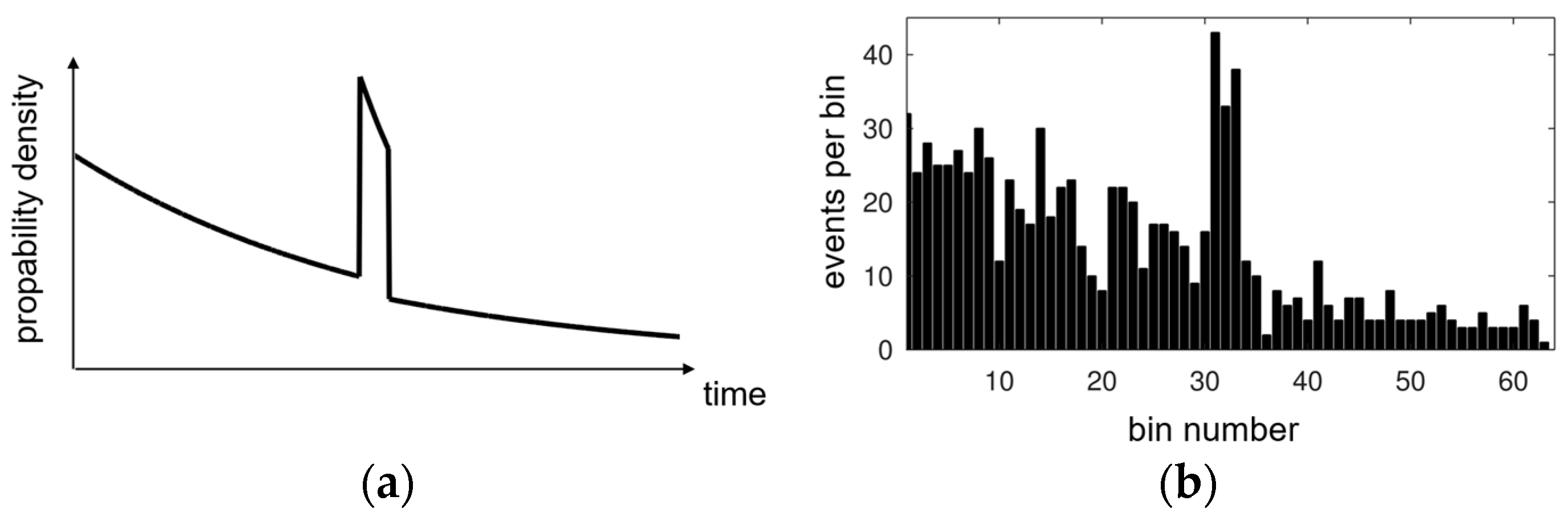
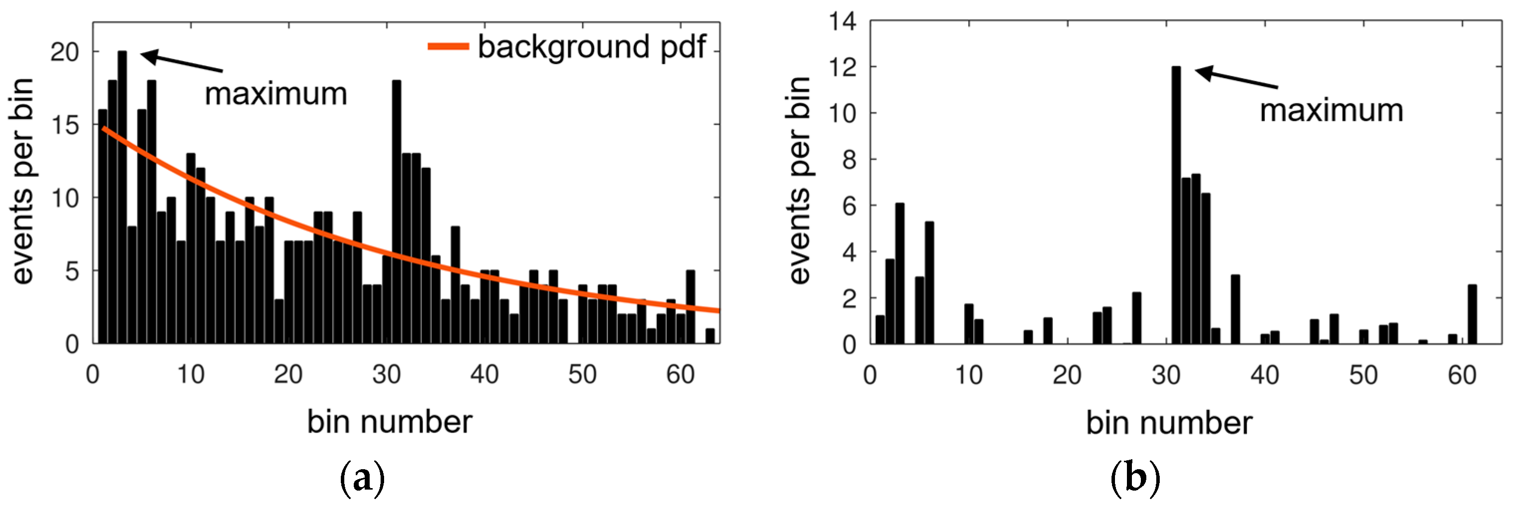
2.2. Probability Density Function
2.3. Signal-to-Noise Ratio
2.4. Laser Pulse Detection Probability
3. Results
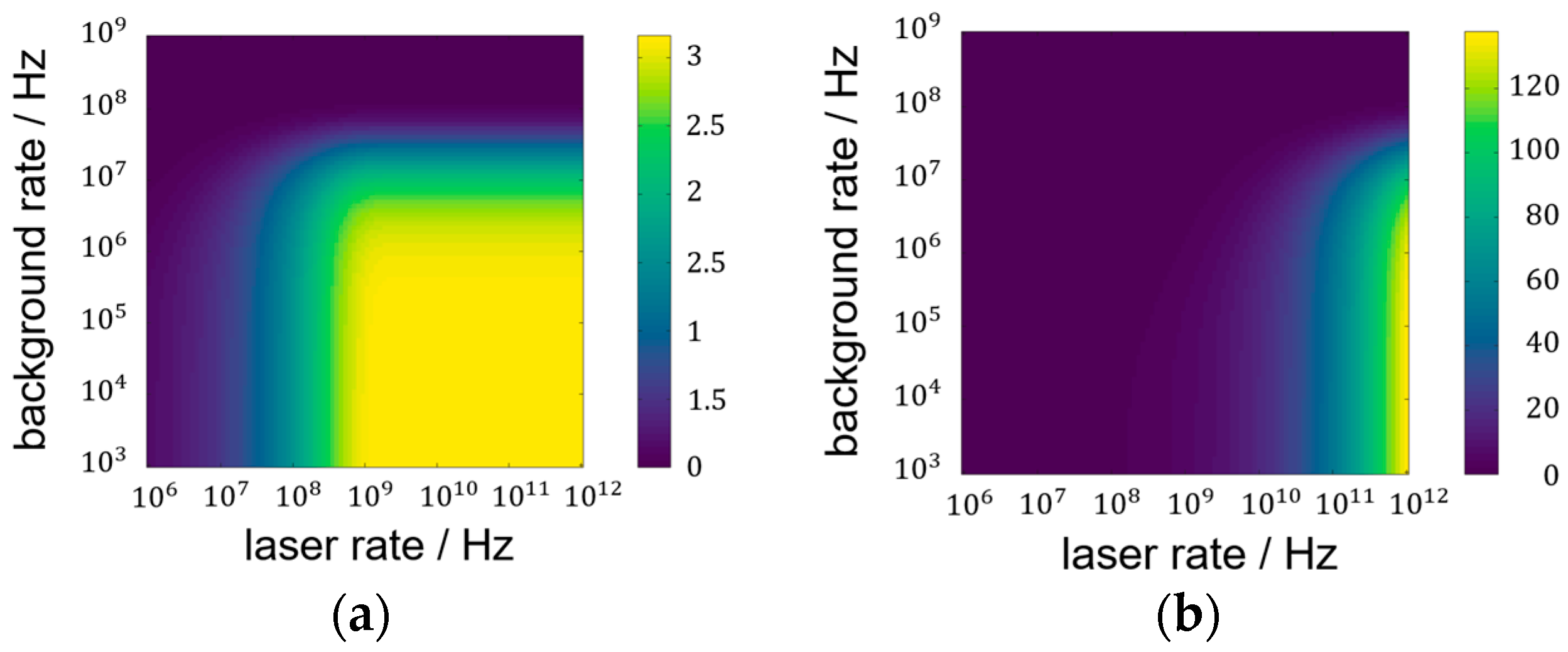
3.1. SNR Analysis
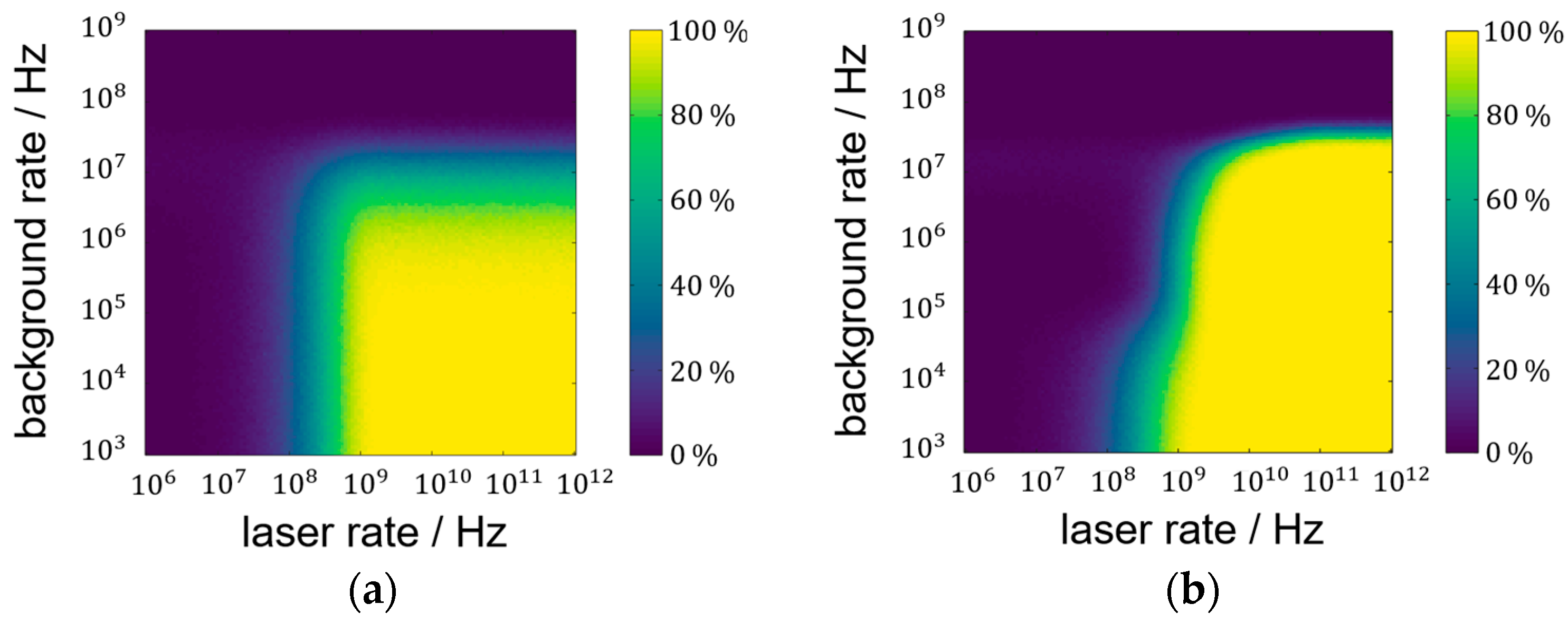
3.2. Laser Pulse Detection Probability Analysis
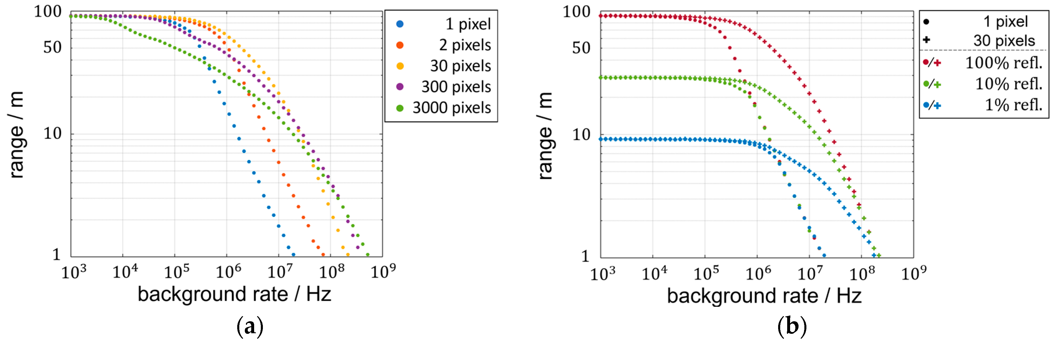
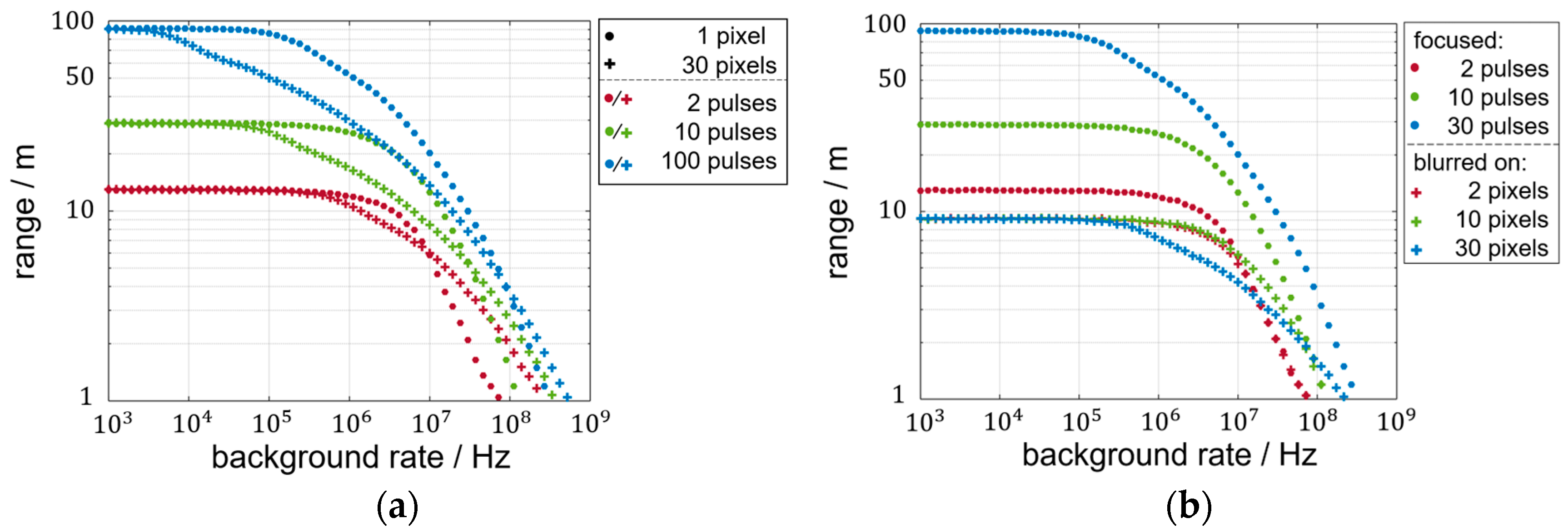
3.3. Range Limitations
4. Discussion
Author Contributions
Funding
Institutional Review Board Statement
Informed Consent Statement
Data Availability Statement
Conflicts of Interest
Abbreviations
| LiDAR | Light detection and ranging |
| SPAD | Single photon avalanche diode |
| ToF | Time-of-flight |
| TDC | Time to digital converter |
| SNR | Signal-to-noise ratio |
| FoV | Field of view |
| Probability density function | |
| LPDP | Lase pulse detection probability |
| SiPM | Silicon photomultiplier |
References
- Villa, F.; Severini, F.; Madonini, F.; Zappa, F. SPADs and SiPMs Arrays for Long-Range High-Speed Light Detection and Ranging (LiDAR). Sensors 2021, 21, 3839. [Google Scholar] [CrossRef] [PubMed]
- Makino, K.; Fujita, T.; Hashi, T.; Adachi, S.; Nakamura, S.; Yamamoto, K.; Baba, T.; Suzuki, Y. Development of an InGaAs SPAD 2D array for flash LIDAR. In Proceedings of the Quantum Sensing and Nano Electronics and Photonics XV, San Francisco, CA, USA, 28 January–2 February 2018; Razeghi, M., Brown, G.J., Leo, G., Lewis, J.S., Eds.; SPIE: Bellingham, WA, USA, 2018; p. 19, ISBN 9781510615656. [Google Scholar]
- Manuzzato, E.; Tontini, A.; Seljak, A.; Perenzoni, M. A 64 times 64—Pixel Flash LiDAR SPAD Imager with Distributed Pixel-to-Pixel Correlation for Background Rejection, Tunable Automatic Pixel Sensitivity and First-Last Event Detection Strategies for Space Applications. In Proceedings of the 2022 IEEE International Solid-State Circuits Conference (ISSCC), San Francisco, CA, USA, 20–26 February 2022; IEEE: Piscataway, NJ, USA, 2022; pp. 96–98, ISBN 978-1-6654-2800-2. [Google Scholar]
- Padmanabhan, P.; Zhang, C.; Charbon, E. Modeling and Analysis of a Direct Time-of-Flight Sensor Architecture for LiDAR Applications. Sensors 2019, 19, 5464. [Google Scholar] [CrossRef] [PubMed]
- Burkard, R.; Viga, R.; Ruskowski, J.; Grabmaier, A. Generalized comparison of the accessible emission limits of flash- and scanning LiDAR-systems. In Proceedings of the SMACD/PRIME 2021: International Conference on SMACD and 16th Conference on PRIME, Online, 19–22 July 2021; pp. 292–295. [Google Scholar]
- Lemmetti, J.; Sorri, N.; Kallioniemi, I.; Melanen, P.; Uusimaa, P. Long-range all-solid-state flash LiDAR sensor for autonomous driving. In Proceedings of the High-Power Diode Laser Technology XIX, Online, 6–12 March 2021; Zediker, M.S., Ed.; SPIE: Bellingham, WA, USA, 2021; p. 22, ISBN 9781510641716. [Google Scholar]
- Yoo, H.W.; Druml, N.; Brunner, D.; Schwarzl, C.; Thurner, T.; Hennecke, M.; Schitter, G. MEMS-based lidar for autonomous driving. Elektrotech. Inftech. 2018, 135, 408–415. [Google Scholar] [CrossRef]
- Kasturi, A.; Milanovic, V.; Lovell, D.B.; Hu, F.; Ho, D.; Su, Y.; Ristic, L. Comparison of MEMS mirror LiDAR architectures. In Proceedings of the MOEMS and Miniaturized Systems, San Francisco, CA, USA, 1–6 February 2020; Piyawattanametha, W., Park, Y.-H., Zappe, H., Eds.; SPIE: Bellingham, WA, USA, 2020; p. 31, ISBN 9781510633490. [Google Scholar]
- Noda, S.; Tanahashi, Y.; Tanimoto, R.; Koutsuka, Y.; Kitano, K.; Takahashi, K.; Muramatsu, E.; Kawabata, C. Development of coaxial 3D-LiDAR systems using MEMS scanners for automotive applications. In Proceedings of the Optical Data Storage 2018: Industrial Optical Devices and Systems, San Diego, CA, USA, 19–23 August 2018; Katayama, R., Takashima, Y., Eds.; SPIE: Bellingham, WA, USA, 2018; p. 14, ISBN 9781510620858. [Google Scholar]
- Wang, Y.; Tang, P.; Shen, L.; Pu, S. LiDAR System Using MEMS Scanner-Based Coaxial Optical Transceiver. In Proceedings of the 2020 IEEE 5th Optoelectronics Global Conference (OGC), Shenzhen, China, 7–11 September 2020; IEEE: Piscataway, NJ, USA, 2020; pp. 166–168, ISBN 978-1-7281-9860-6. [Google Scholar]
- Xu, F.; Qiao, D.; Song, X.; Zheng, W.; He, Y.; Fan, Q. A Semi-coaxial MEMS-based LiDAR. In Proceedings of the IECON 2019—45th Annual Conference of the IEEE Industrial Electronics Society, Lisbon, Portugal, 14–17 October 2019; IEEE: Piscataway, NJ, USA, 2019; pp. 6726–6731, ISBN 978-1-7281-4878-6. [Google Scholar]
- Sakata, R.; Ishizaki, K.; de Zoysa, M.; Fukuhara, S.; Inoue, T.; Tanaka, Y.; Iwata, K.; Hatsuda, R.; Yoshida, M.; Gelleta, J.; et al. Dually modulated photonic crystals enabling high-power high-beam-quality two-dimensional beam scanning lasers. Nat. Commun. 2020, 11, 3487. [Google Scholar] [CrossRef]
- Sakata, R.; Ishizaki, K.; de Zoysa, M.; Kitamura, K.; Inoue, T.; Gelleta, J.; Noda, S. Photonic-crystal surface-emitting lasers with modulated photonic crystals enabling 2D beam scanning and various beam pattern emission. Appl. Phys. Lett. 2023, 122, 130503. [Google Scholar] [CrossRef]
- Noda, S.; Yoshida, M.; Inoue, T.; de Zoysa, M.; Ishizaki, K.; Sakata, R. Photonic-crystal surface-emitting lasers. Nat. Rev. Electr. Eng. 2024, 1, 802–814. [Google Scholar] [CrossRef]
- Zhuo, S.; Xia, T.; Zhao, L.; Sun, M.; Wu, Y.; Wang, L.; Yu, H.; Xu, J.; Wang, J.; Lin, Z.; et al. Solid-State dToF LiDAR System Using an Eight-Channel Addressable, 20-W/Ch Transmitter, and a 128 × 128 SPAD Receiver With SNR-Based Pixel Binning and Resolution Upscaling. IEEE J. Solid-State Circuits 2023, 58, 757–770. [Google Scholar] [CrossRef]
- Lei, Y.; Zhang, L.; Yu, Z.; Xue, Y.; Ren, Y.; Sun, X. Si Photonics FMCW LiDAR Chip with Solid-State Beam Steering by Interleaved Coaxial Optical Phased Array. Micromachines 2023, 14, 1001. [Google Scholar] [CrossRef] [PubMed]
- Muntaha, S.T.; Hokkanen, A.; Harjanne, M.; Cherchi, M.; Roussey, M.; Aalto, T. Optical beam steering and distance measurement experiments through an optical phased array and a 3D printed lens. Opt. Express 2025, 33, 3685. [Google Scholar] [CrossRef]
- Poulton, C.V.; Byrd, M.J.; Russo, P.; Timurdogan, E.; Khandaker, M.; Vermeulen, D.; Watts, M.R. Long-Range LiDAR and Free-Space Data Communication With High-Performance Optical Phased Arrays. IEEE J. Select. Topics Quantum Electron. 2019, 25, 1–8. [Google Scholar] [CrossRef]
- Lee, J.; Shin, D.; Jang, B.; Byun, H.; Lee, C.; Shin, C.; Hwang, I.; Shim, D.; Lee, E.; Kim, J.; et al. Single-Chip Beam Scanner with Integrated Light Source for Real-Time Light Detection and Ranging. In Proceedings of the 2020 IEEE International Electron Devices Meeting (IEDM), San Francisco, CA, USA, 12–18 December 2020; IEEE: Piscataway, NJ, USA, 2020; pp. 7.2.1–7.2.4, ISBN 978-1-7281-8888-1. [Google Scholar]
- Sesta, V.; Severini, F.; Villa, F.; Lussana, R.; Zappa, F.; Nakamuro, K.; Matsui, Y. Spot Tracking and TDC Sharing in SPAD Arrays for TOF LiDAR. Sensors 2021, 21, 2936. [Google Scholar] [CrossRef] [PubMed]
- Burkard, R.; Ligges, M.; Merten, A.; Sandner, T.; Viga, R.; Grabmaier, A. Histogram formation and noise reduction in biaxial MEMS-based SPAD light detection and ranging systems. J. Opt. Microsyst. 2022, 2, 011005. [Google Scholar] [CrossRef]
- Haase, J.F.; Grollius, S.; Grosse, S.; Buchner, A.; Ligges, M. A 32x24 pixel SPAD detector system for LiDAR and quantum imaging. In Proceedings of the Photonic Instrumentation Engineering VIII, Online, 6–12 March 2021; Soskind, Y., Busse, L.E., Eds.; SPIE: Piscataway, NJ, USA, 2021; p. 20, ISBN 9781510642218. [Google Scholar]
- Henderson, R.K.; Johnston, N.; Hutchings, S.W.; Gyongy, I.; Abbas, T.A.; Dutton, N.; Tyler, M.; Chan, S.; Leach, J. 5.7 A 256×256 40nm/90nm CMOS 3D-Stacked 120dB Dynamic-Range Reconfigurable Time-Resolved SPAD Imager. In Proceedings of the 2019 IEEE International Solid- State Circuits Conference (ISSCC), San Francisco, CA, USA, 17–21 February 2019; IEEE: Piscataway, NJ, USA, 2019; pp. 106–108, ISBN 978-1-5386-8531-0. [Google Scholar]
- Padmanabhan, P.; Zhang, C.; Cazzaniga, M.; Efe, B.; Ximenes, A.R.; Lee, M.-J.; Charbon, E. 7.4 A 256×128 3D-Stacked (45nm) SPAD FLASH LiDAR with 7-Level Coincidence Detection and Progressive Gating for 100m Range and 10klux Background Light. In Proceedings of the 2021 IEEE International Solid-State Circuits Conference (ISSCC), San Francisco, CA, USA, 13–22 February 2021; IEEE: Piscataway, NJ, USA, 2021; pp. 111–113, ISBN 978-1-7281-9549-0. [Google Scholar]
- Henderson, R.K.; Johnston, N.; Della Mattioli Rocca, F.; Chen, H.; Day-Uei Li, D.; Hungerford, G.; Hirsch, R.; Mcloskey, D.; Yip, P.; Birch, D.J.S. A 192 times 128 Time Correlated SPAD Image Sensor in 40-nm CMOS Technology. IEEE J. Solid-State Circuits 2019, 54, 1907–1916. [Google Scholar] [CrossRef]
- Buchner, A.; Hadrath, S.; Burkard, R.; Kolb, F.M.; Ruskowski, J.; Ligges, M.; Grabmaier, A. Analytical Evaluation of Signal-to-Noise Ratios for Avalanche- and Single-Photon Avalanche Diodes. Sensors 2021, 21, 2887. [Google Scholar] [CrossRef] [PubMed]
- Leitel, R.; Dannberg, P.; Seise, B.; Brüning, R.; Grosse, S.; Ligges, M. Enhancement of SPAD-camera sensitivity by molded microlens arrays. In Proceedings of the Optical Sensing and Detection VIII, Strasbourg, France, 7–12 April 2024; Berghmans, F., Zergioti, I., Eds.; SPIE: Bellingham, WA, USA, 2024; p. 71, ISBN 9781510673168. [Google Scholar]
- IEC 60825-1:2014; Safety of Laser Products—Part 1: Equipment Classification and Requirements. International Electrotechnical Commission: Berlin, Germany, 2014.
- Al Abbas, T.; Dutton, N.A.; Almer, O.; Finlayson, N.; Della Rocca, F.M.; Henderson, R. A CMOS SPAD Sensor With a Multi-Event Folded Flash Time-to-Digital Converter for Ultra-Fast Optical Transient Capture. IEEE Sensors J. 2018, 18, 3163–3173. [Google Scholar] [CrossRef]
- Fu, Y.-H.; Zhao, Z.-Y.; Zhao, Z.; Li, J.-C.; Chang, Y.-C. A SPAD Readout Circuit Based on Column-Level Event-Driven Time-to-Digital Converter. In Proceedings of the 2022 IEEE 16th International Conference on Solid-State & Integrated Circuit Technology (ICSICT), Nangjing, China, 25–28 October 2022; IEEE: Piscataway, NJ, USA, 2022; pp. 1–3, ISBN 978-1-6654-6906-7. [Google Scholar]
- Sesta, V.; Incoronato, A.; Madonini, F.; Villa, F. Time-to-digital converters and histogram builders in SPAD arrays for pulsed-LiDAR. Measurement 2023, 212, 112705. [Google Scholar] [CrossRef]


| Light Type | Focused Setup: Rate per Pixel | Lens-Less Setup: Rate per Pixel | Blurred Setup: Rate per Pixel |
|---|---|---|---|
| Background | |||
| Laser signal | * |
Disclaimer/Publisher’s Note: The statements, opinions and data contained in all publications are solely those of the individual author(s) and contributor(s) and not of MDPI and/or the editor(s). MDPI and/or the editor(s) disclaim responsibility for any injury to people or property resulting from any ideas, methods, instructions or products referred to in the content. |
© 2025 by the authors. Licensee MDPI, Basel, Switzerland. This article is an open access article distributed under the terms and conditions of the Creative Commons Attribution (CC BY) license (https://creativecommons.org/licenses/by/4.0/).
Share and Cite
Albert, K.; Ligges, M.; Henschke, A.; Ruskowski, J.; De Zoysa, M.; Noda, S.; Grabmaier, A. Performance Comparison of Multipixel Biaxial Scanning Direct Time-of-Flight Light Detection and Ranging Systems With and Without Imaging Optics. Sensors 2025, 25, 3229. https://doi.org/10.3390/s25103229
Albert K, Ligges M, Henschke A, Ruskowski J, De Zoysa M, Noda S, Grabmaier A. Performance Comparison of Multipixel Biaxial Scanning Direct Time-of-Flight Light Detection and Ranging Systems With and Without Imaging Optics. Sensors. 2025; 25(10):3229. https://doi.org/10.3390/s25103229
Chicago/Turabian StyleAlbert, Konstantin, Manuel Ligges, Andre Henschke, Jennifer Ruskowski, Menaka De Zoysa, Susumu Noda, and Anton Grabmaier. 2025. "Performance Comparison of Multipixel Biaxial Scanning Direct Time-of-Flight Light Detection and Ranging Systems With and Without Imaging Optics" Sensors 25, no. 10: 3229. https://doi.org/10.3390/s25103229
APA StyleAlbert, K., Ligges, M., Henschke, A., Ruskowski, J., De Zoysa, M., Noda, S., & Grabmaier, A. (2025). Performance Comparison of Multipixel Biaxial Scanning Direct Time-of-Flight Light Detection and Ranging Systems With and Without Imaging Optics. Sensors, 25(10), 3229. https://doi.org/10.3390/s25103229