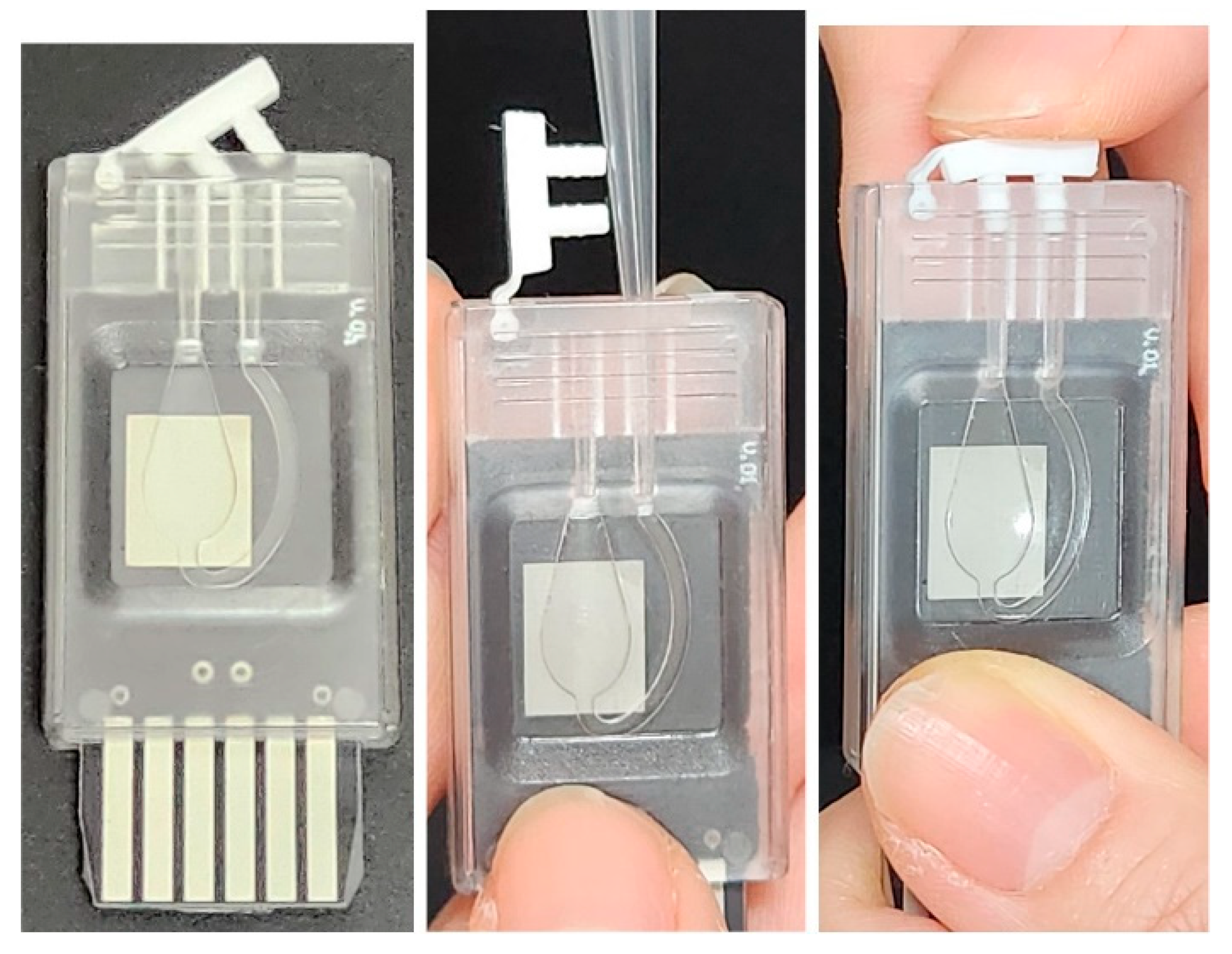
Figure 1.
PCR chip and reagent injection procedure. The chip dimensions are approximately 22 mm (width) × 50 mm (length) × 5 mm (thickness).
Figure 1.
PCR chip and reagent injection procedure. The chip dimensions are approximately 22 mm (width) × 50 mm (length) × 5 mm (thickness).
Figure 2.
Hardware functional block diagram.
Figure 2.
Hardware functional block diagram.
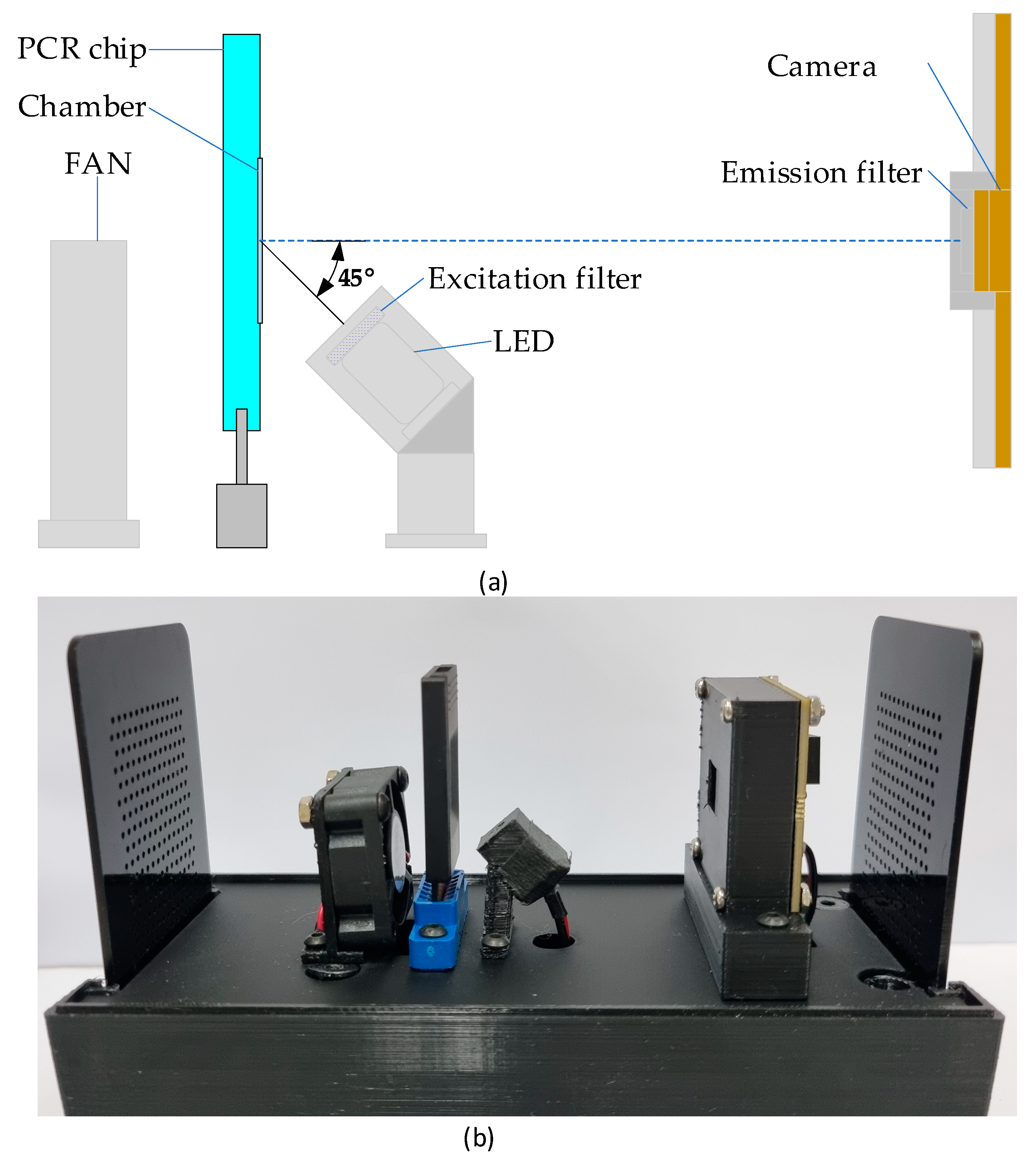
Figure 3.
The system block diagram (a) and its implementation picture (b). The assembled system measures approximately 80 mm (width) × 155 mm (length) × 130 mm (height).
Figure 3.
The system block diagram (a) and its implementation picture (b). The assembled system measures approximately 80 mm (width) × 155 mm (length) × 130 mm (height).
Figure 4.
Software architecture.
Figure 4.
Software architecture.
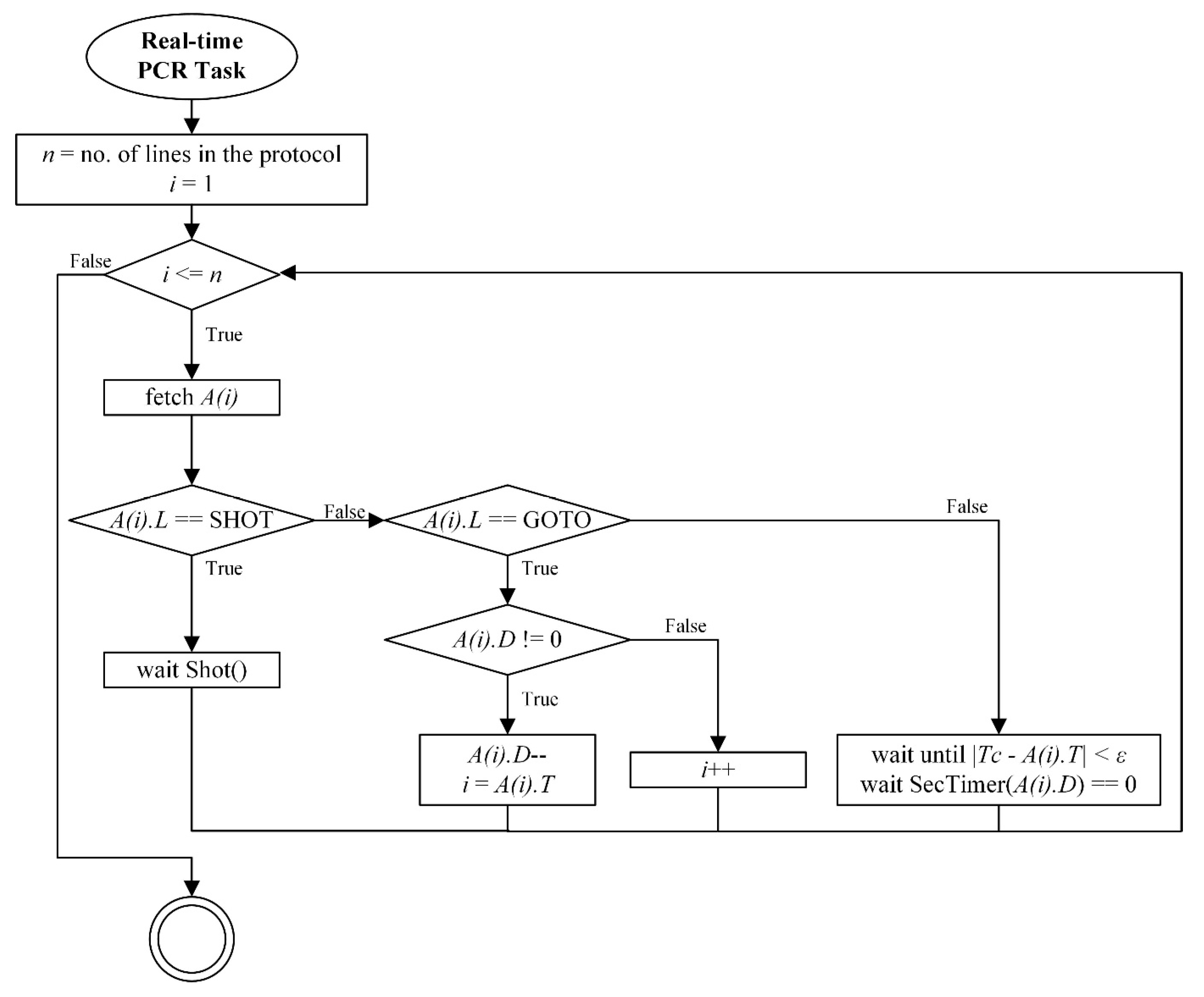
Figure 5.
Real-time PCR protocol processing flow diagram.
Figure 5.
Real-time PCR protocol processing flow diagram.
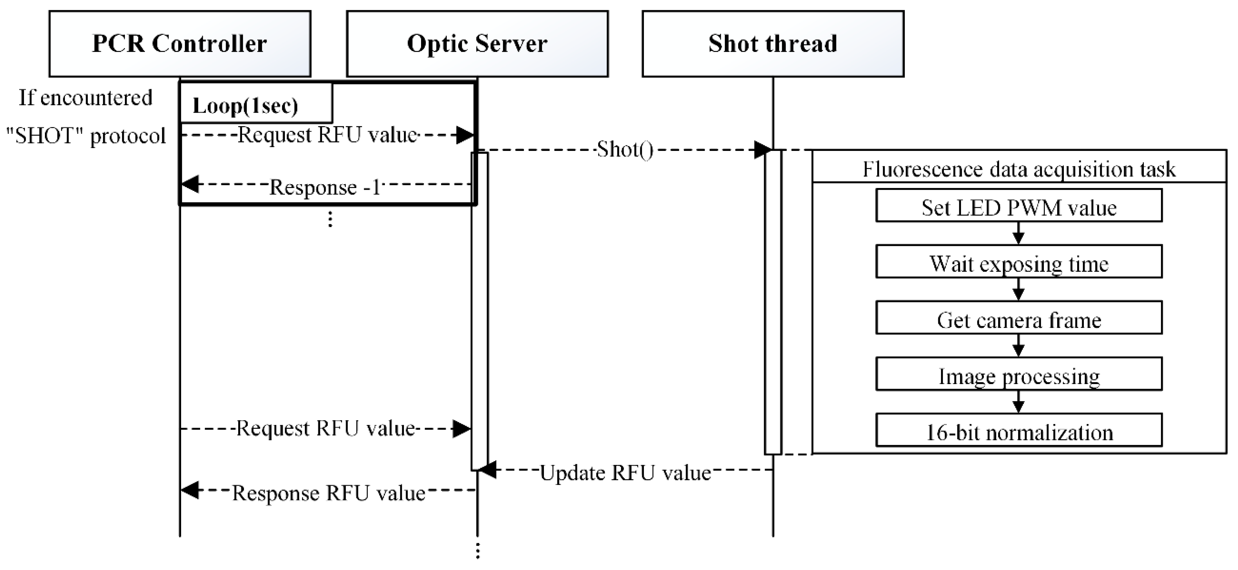
Figure 6.
“SHOT” command processing.
Figure 6.
“SHOT” command processing.
Figure 7.
Timing sequence for acquiring a fully illuminated fluorescence frame using asynchronous LED activation and camera capture. The LED is turned on by the shot thread (top layer) and remains on long enough to ensure the camera captures a frame (e.g., f1) that is fully exposed to the excitation light. Due to the asynchronous nature of the shot thread, camera thread, and frame transfer, the LED must remain on for a sufficient duration to ensure reliable image acquisition.
Figure 8.
Average fluorescence intensity trends across 100 repeated image sequence acquisitions for different exposure times. Each curve shows how the mean brightness evolves over time after LED activation. The vertical axis represents relative intensity, and the horizontal axis represents time. The point at which brightness stabilizes was used to determine the minimum required LED-on duration for each exposure condition.
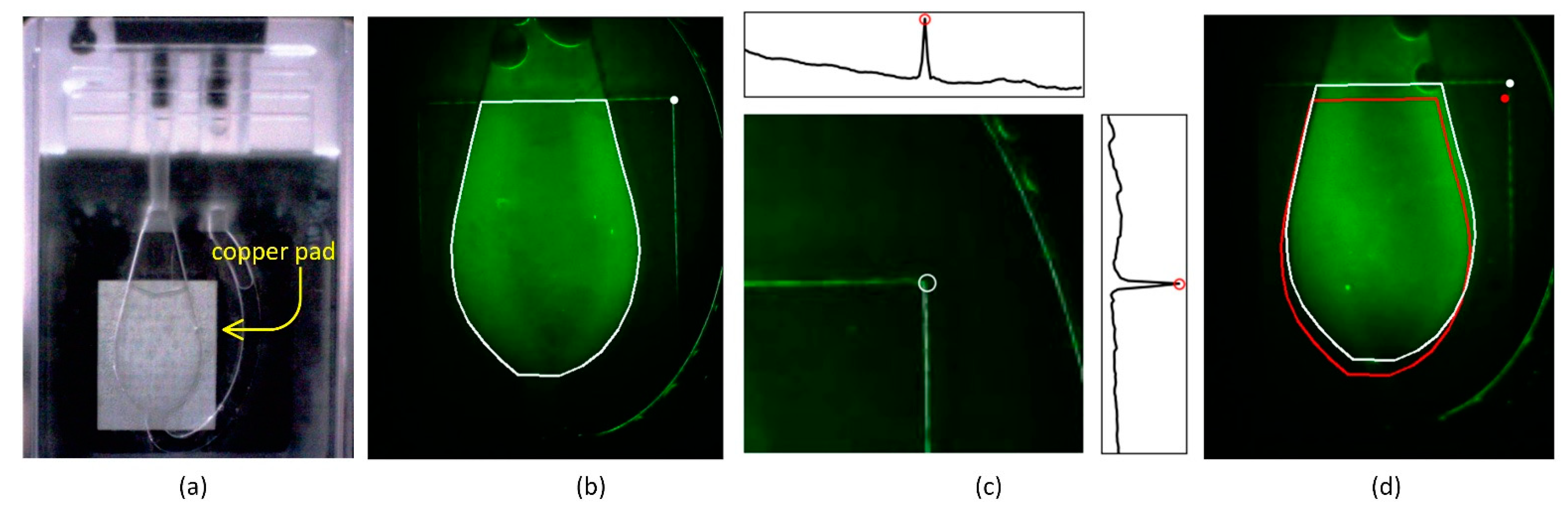
Figure 9.
ROI localization using copper pad edge detection for reliable fluorescence quantification. (a) Image of a PCR chip filled with reagent, showing the chamber and the underlying nickel-coated copper pad used for thermal spreading. (b) Fluorescence image of a chip filled with FAM dye, with the manually defined tight ROI (white outline) and the detected marker point (white circle). (c) Method for detecting the right upper corner of the copper pad using projection peaks in a predefined search area. Insets show distinct horizontal and vertical intensity peaks used to locate the corner, marked with a white circle. (d) Comparison between a misaligned tight ROI (red outline) based on average marker position and a corrected ROI (white outline) relocated using the detected corner. The corrected ROI better encloses the chamber region, reducing positional error across devices.
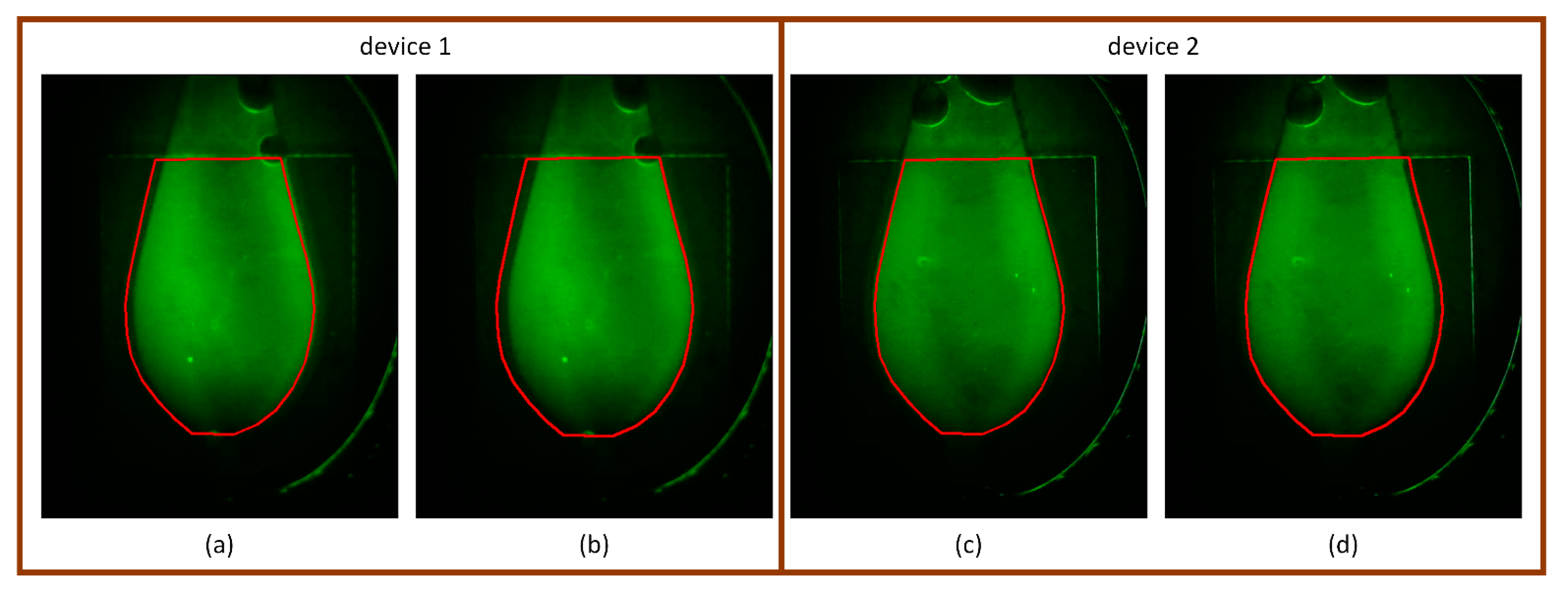
Figure 10.
Comparison of tight and dilated ROIs on fluorescence images with large marker deviation. (a,b) Device 1: The tight ROI fails to fully capture the fluorescent chamber due to horizontal misalignment, whereas the dilated ROI successfully covers the entire chamber region. (c,d) Device 2: Although the tight ROI is relatively well-aligned, minor misalignment is still visible. The dilated ROI corrects this with a slight trade-off of including additional background signal.
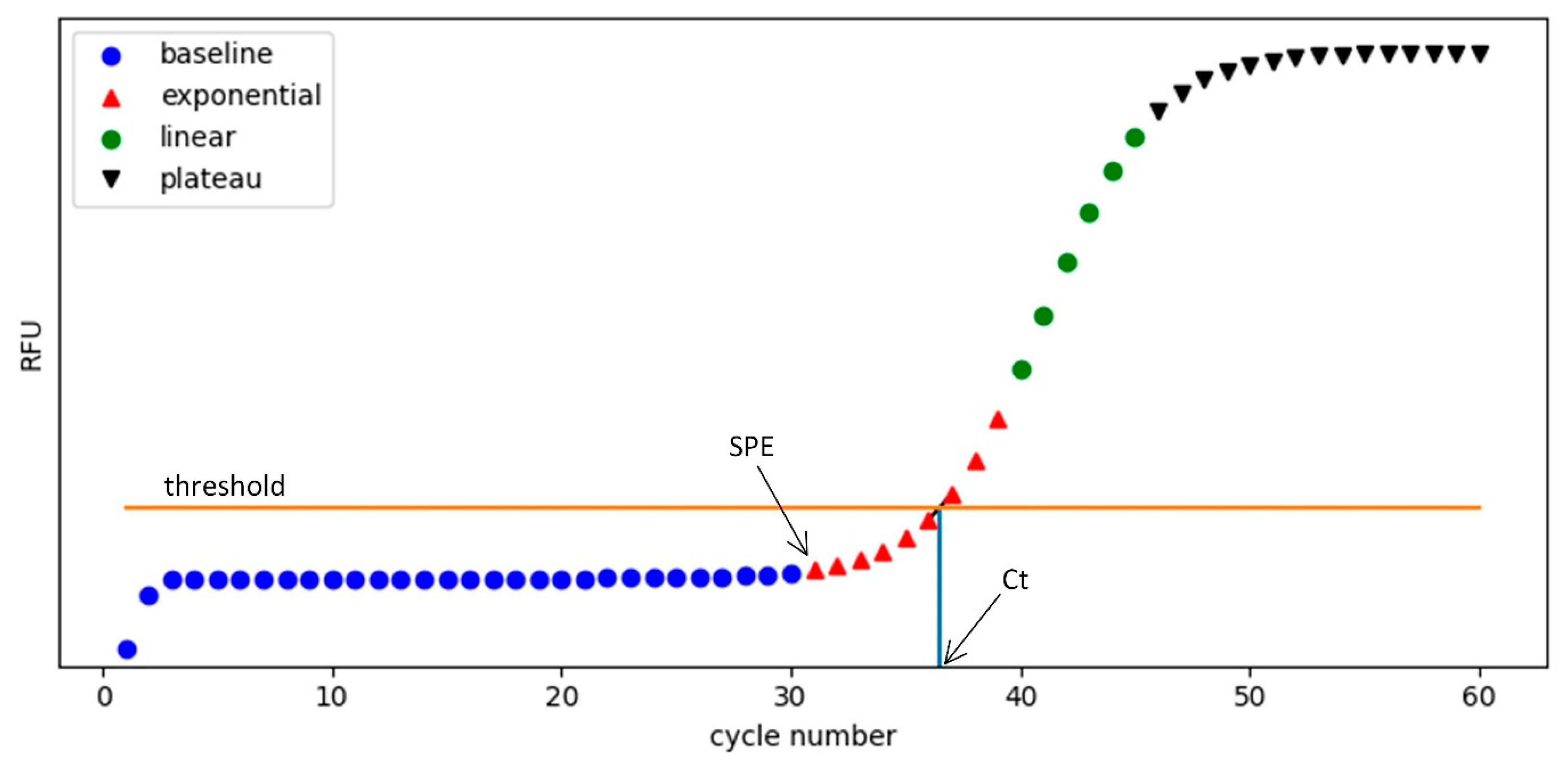
Figure 11.
Characteristic phases of a real-time PCR amplification curve. The curve is divided into four segments: baseline (blue circles), exponential (red triangles), linear (green circles), and plateau (black inverted triangles). The horizontal orange line represents the signal threshold level for Ct determination. The start point of the exponential phase (SPE) marks the onset of rapid signal increase, while the cycle threshold (Ct) is the point where the fluorescence curve crosses the threshold. The Ct value is used as a diagnostic criterion: samples with Ct values lower than a preset decision threshold are considered positive.
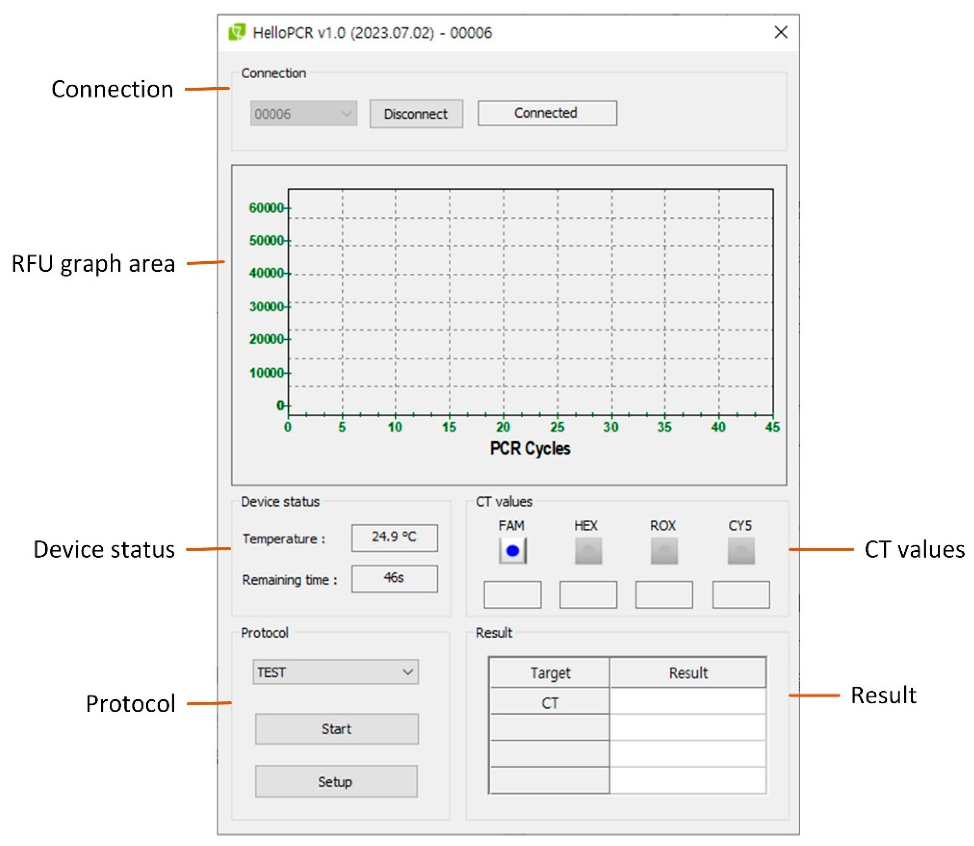
Figure 12.
Main user interface of the PCR system. The UI contains six main control groups: (1) Connection, (2) RFU graph area, (3) Device status, (4) CT values, (5) Protocol control, and (6) Result panel.
Figure 12.
Main user interface of the PCR system. The UI contains six main control groups: (1) Connection, (2) RFU graph area, (3) Device status, (4) CT values, (5) Protocol control, and (6) Result panel.
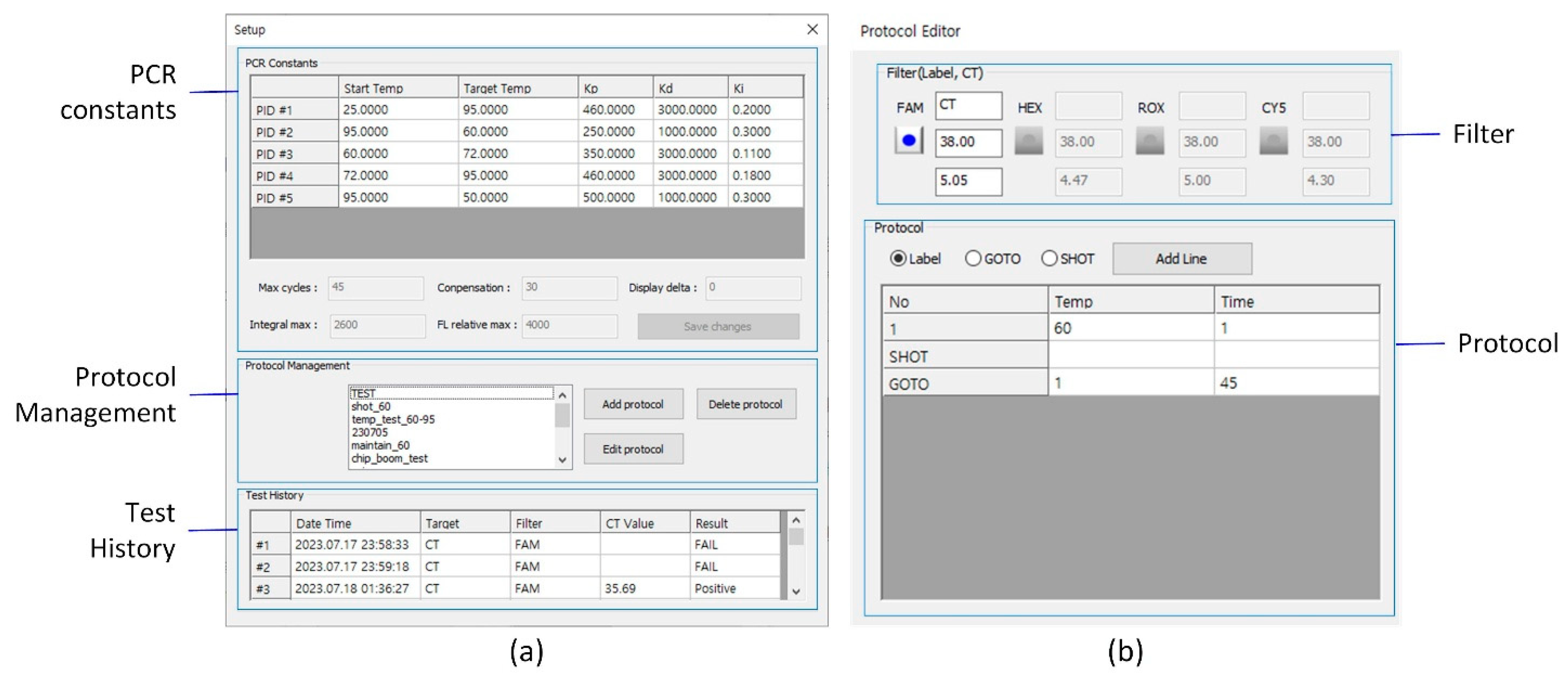
Figure 13.
(a) Setup UI for configuring PCR constants, managing protocols, and accessing test history. (b) Protocol Editor UI for defining thermal cycling parameters and fluorescence channel settings, including the decision threshold for result classification and the signal threshold for Ct determination.
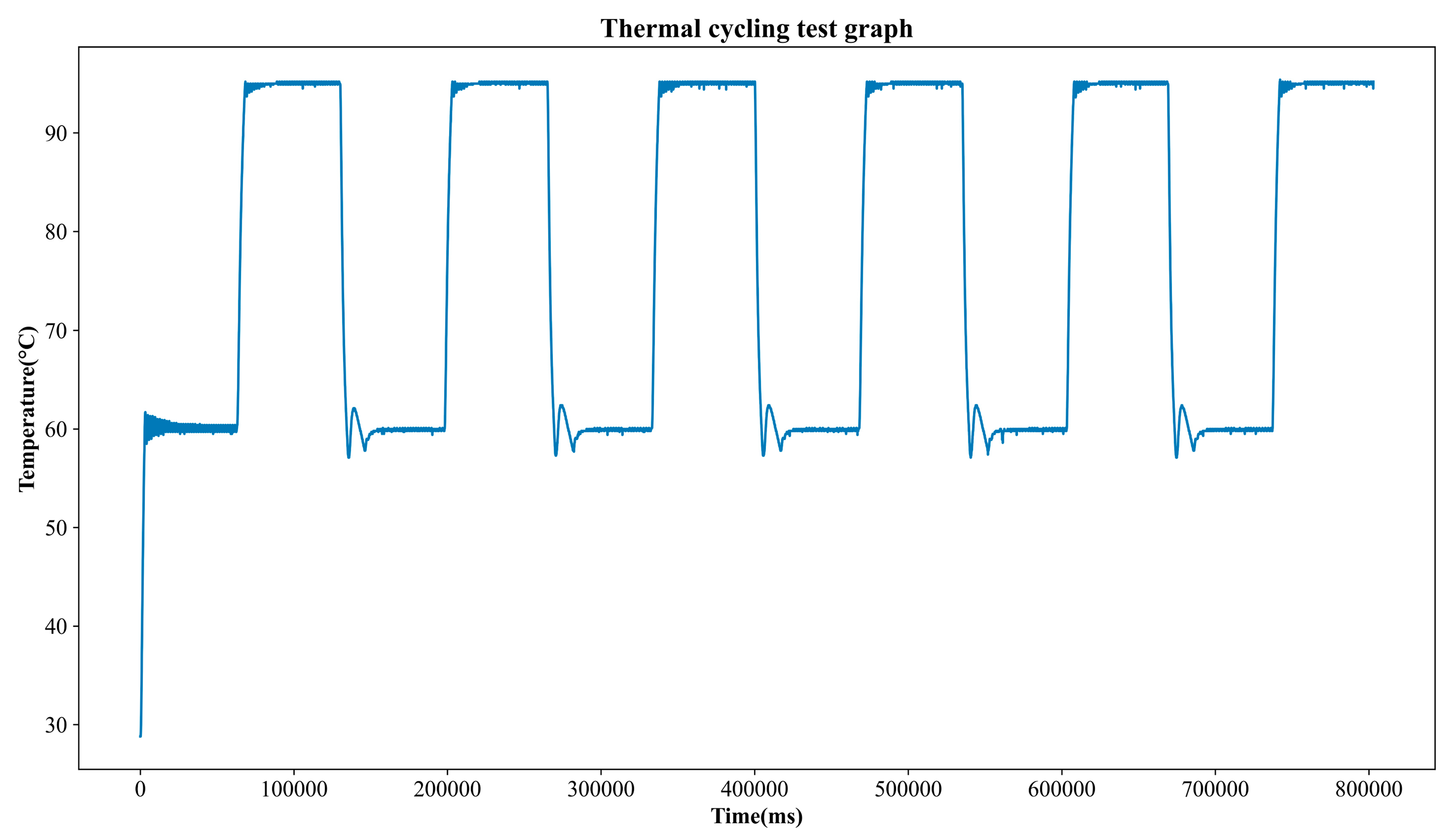
Figure 14.
Thermal cycling test temperature profile.
Figure 14.
Thermal cycling test temperature profile.
Figure 15.
Fluorescence images of PCR chips filled with distilled water (DW) and 1 pM/µL FAM solution, captured at camera gain settings of 0 and 50. The images illustrate the contrast between background and amplified-like fluorescence signals, with no saturation observed at either gain level.
Figure 15.
Fluorescence images of PCR chips filled with distilled water (DW) and 1 pM/µL FAM solution, captured at camera gain settings of 0 and 50. The images illustrate the contrast between background and amplified-like fluorescence signals, with no saturation observed at either gain level.
Figure 16.
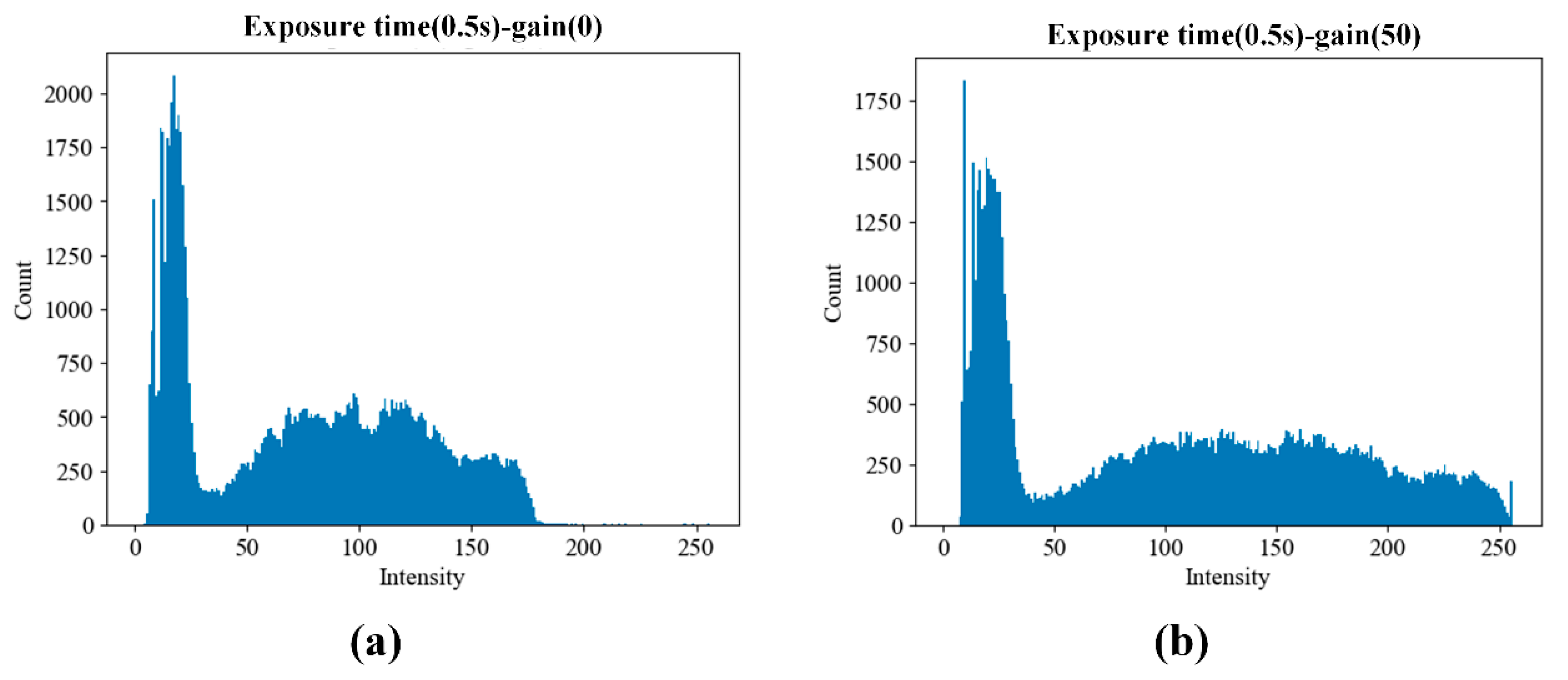
Cumulative histograms of pixel intensity within the region of interest (ROI) from PCR chips filled with 1 pM/µL FAM solution. Data were acquired using five replicate chips under two gain conditions: (a) gain = 0 and (b) gain = 50. The results confirm that both settings avoid pixel saturation while allowing sufficient signal differentiation for downstream quantification.
Figure 16.
Cumulative histograms of pixel intensity within the region of interest (ROI) from PCR chips filled with 1 pM/µL FAM solution. Data were acquired using five replicate chips under two gain conditions: (a) gain = 0 and (b) gain = 50. The results confirm that both settings avoid pixel saturation while allowing sufficient signal differentiation for downstream quantification.
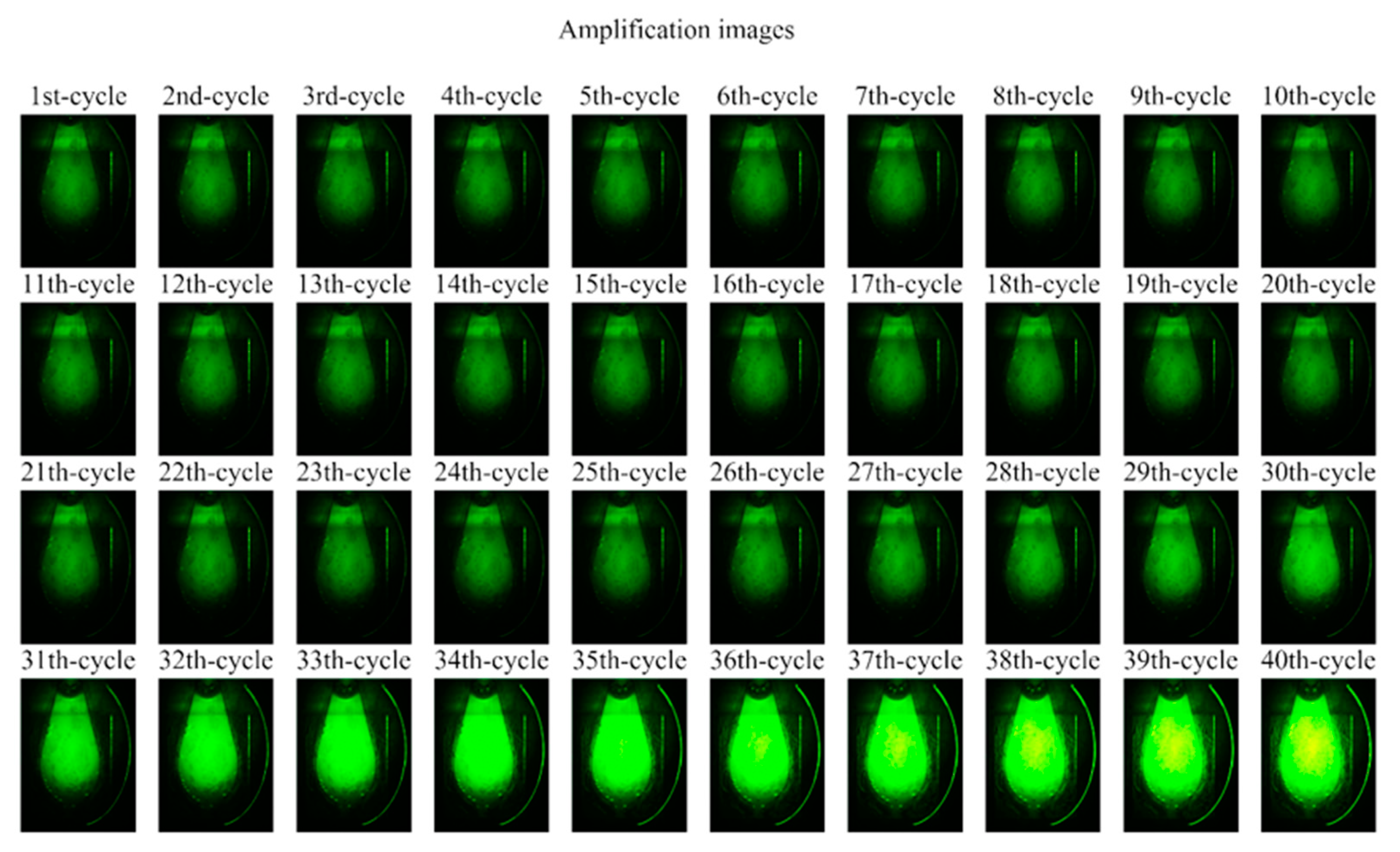
Figure 17.
Time-lapse fluorescence images of the PCR chip chamber acquired at each PCR cycle. Images were captured with a camera exposure time of 0.5 s and gain of 30 after the extension step at 60 °C. Brightness and contrast were enhanced for visibility. Increased fluorescence intensity became noticeable starting from cycle 26.
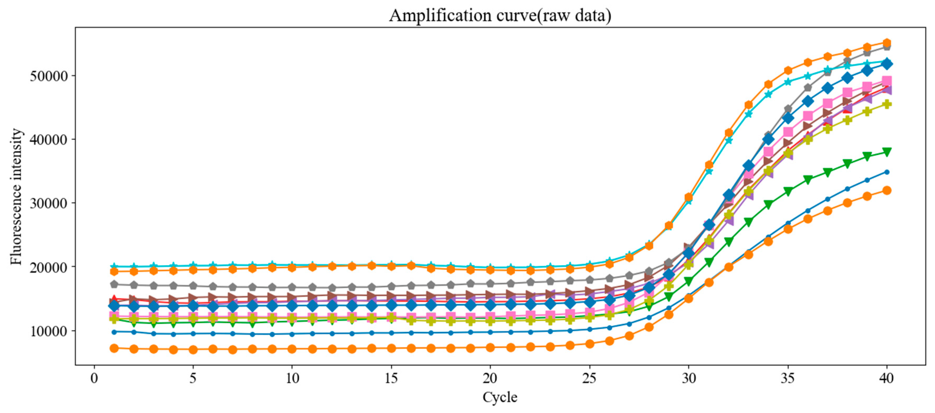
Figure 18.
Raw fluorescence amplification curves from 12 replicate PCR runs using the same concentration of Chlamydia trachomatis DNA standard. Despite using identical samples, small variations in Ct values were observed, emphasizing the need for proper baseline correction.
Figure 18.
Raw fluorescence amplification curves from 12 replicate PCR runs using the same concentration of Chlamydia trachomatis DNA standard. Despite using identical samples, small variations in Ct values were observed, emphasizing the need for proper baseline correction.
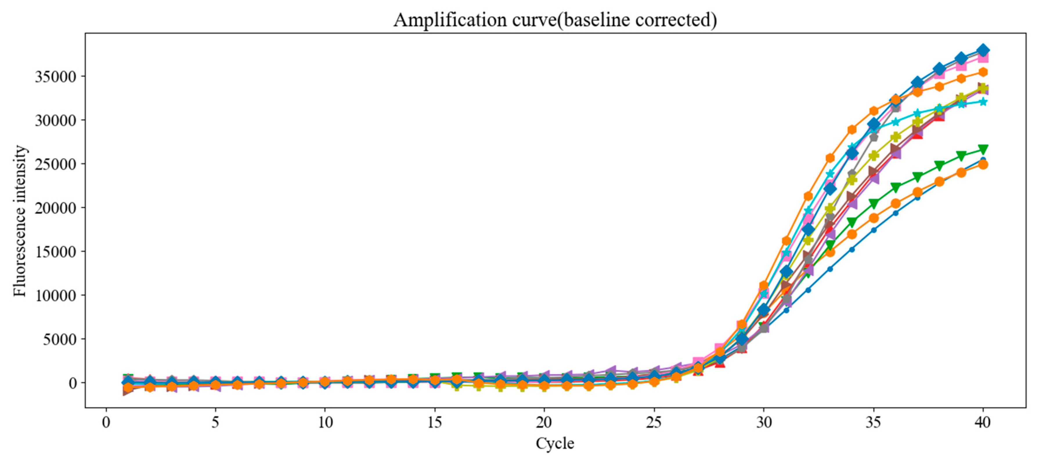
Figure 19.
Fluorescence amplification curves after applying fixed-mean baseline correction to the data shown in
Figure 18. The correction improves alignment and consistency of the curves, reducing Ct variability across replicate tests.
Figure 19.
Fluorescence amplification curves after applying fixed-mean baseline correction to the data shown in
Figure 18. The correction improves alignment and consistency of the curves, reducing Ct variability across replicate tests.
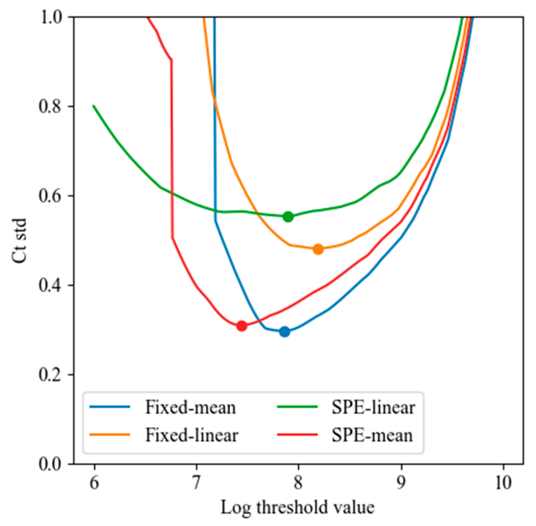
Figure 20.
Minimum Ct standard deviation obtained by varying the threshold value (log scale) for each of the four baseline correction methods: fixed-mean, fixed-linear, SPE-mean, and SPE-linear. Mean-based methods outperformed linear regression methods, with the fixed-mean method achieving the lowest Ct variability (σ < 0.3 cycles).
Table 1.
An example of real-time PCR protocol.
Table 1.
An example of real-time PCR protocol.
| Label | Temperature (°C) | Duration (s) |
|---|
| 1 | 95 | 300 |
| 2 | 95 | 30 |
| 3 | 55 | 30 |
| 4 | 72 | 30 |
| SHOT | - | - |
| GOTO | 2 | 34 |
| 5 | 72 | 180 |
Table 2.
Minimum LED-on time required to obtain stable fluorescence intensity, based on 100 repeated measurements per exposure time. The stable start time indicates the earliest point where signal intensity no longer increases. The ratio shows the required LED-on duration relative to the camera exposure time.
| Exposure Time (s) | Stable Start Time (s) | Ratio |
|---|
| 0.5 | 1.18 | 2.4 |
| 0.25 | 0.6 | 2.4 |
| 0.125 | 0.36 | 2.9 |
| 0.0625 | 0.28 | 4.5 |
Table 3.
Experimental and device-level deviations in copper pad corner location (in pixels). Data were collected from six insertions per device using chips with clearly visible copper outlines. “Range” refers to the maximum deviation observed, “MAD” is the mean absolute deviation from the device-specific mean, and σ indicates the standard deviation. Results show that device-to-device variation is significantly greater than experimental variation.
| | x-Range | y-Range | x-MAD | x-MAD | σx | σy |
|---|
| device 1 | 9 | 3 | 6.0 | 2.2 | 3.1 | 1.1 |
| device 2 | 5 | 1 | 2.7 | 0.7 | 1.8 | 0.5 |
| device 1 & 2 | 15 | 21 | 9.2 | 11.3 | 4.1 | 9.1 |
Table 4.
Temperature heating and cooling rate (°C/s).
Table 4.
Temperature heating and cooling rate (°C/s).
| Cycle | 1 | 2 | 3 | 4 | 5 | mean | std |
|---|
| Heating rate | 7.6 | 7.9 | 8.0 | 8.1 | 8.1 | 8.0 | 0.2 |
| Cooling rate | −9.3 | −9.5 | −9.4 | −9.2 | −9.3 | −9.3 | 0.1 |
Table 5.
Mean error and the standard deviation at the steady state (°C).
Table 5.
Mean error and the standard deviation at the steady state (°C).
| Cycle | | 1 | 2 | 3 | 4 | 5 |
|---|
| 95 | mean | 0.04 | 0.05 | 0.05 | 0.05 | 0.05 |
| | std | 0.11 | 0.11 | 0.12 | 0.11 | 0.11 |
| 60 | mean | −0.06 | −0.06 | −0.07 | −0.09 | −0.07 |
| | std | 0.10 | 0.10 | 0.10 | 0.14 | 0.10 |
Table 6.
ROI average intensity values for DW and FAM samples across five PCR chips at camera gains of 0 and 50. Relative gain (FAM−DW)/FAM quantifies signal enhancement due to amplification.
Table 6.
ROI average intensity values for DW and FAM samples across five PCR chips at camera gains of 0 and 50. Relative gain (FAM−DW)/FAM quantifies signal enhancement due to amplification.
| Camera Gain | | chip 1 | chip 2 | chip 3 | chip 4 | chip 5 | mean |
|---|
| 0 | DW | 11.6 | 11.4 | 11.6 | 11.8 | 12.5 | 11.8 |
| FAM | 82.8 | 69.0 | 103.1 | 96.9 | 81.8 | 86.7 |
| Relative gain | 6.1 | 5.1 | 7.9 | 7.2 | 5.6 | 6.4 |
| 50 | DW | 14.0 | 13.7 | 14.0 | 14.4 | 15.0 | 14.2 |
| FAM | 113.5 | 90.1 | 143.9 | 132.1 | 112.2 | 118.4 |
| Relative gain | 7.1 | 5.6 | 9.3 | 8.2 | 6.4 | 7.3 |
Table 7.
Thermal cycling protocol used for the amplification of Chlamydia trachomatis DNA. Labels 1 and 2 correspond to initial activation and denaturation steps, followed by 39 cycles of denaturation (Label 3), annealing/extension (Label 4), and fluorescence capture (SHOT). The GOTO command loops back to Label 3 for repeated cycling.
| Label | Temperature (°C) | Duration (s) |
|---|
| 1 | 50 | 120 |
| 2 | 95 | 600 |
| 3 | 95 | 15 |
| 4 | 60 | 60 |
| SHOT | - | - |
| GOTO | 3 | 39 |


