
Generation of Structural Components for Indoor Spaces from Point Clouds

Abstract
1. Introduction
2. Related Work
2.1. Surface Mesh Generation from Point Clouds
2.2. Plane Extraction
2.3. Graph-Cut-Based Algorithm
3. Methods
3.1. Plane Extraction
3.2. Signed Distance Field Generation
- Step 1:
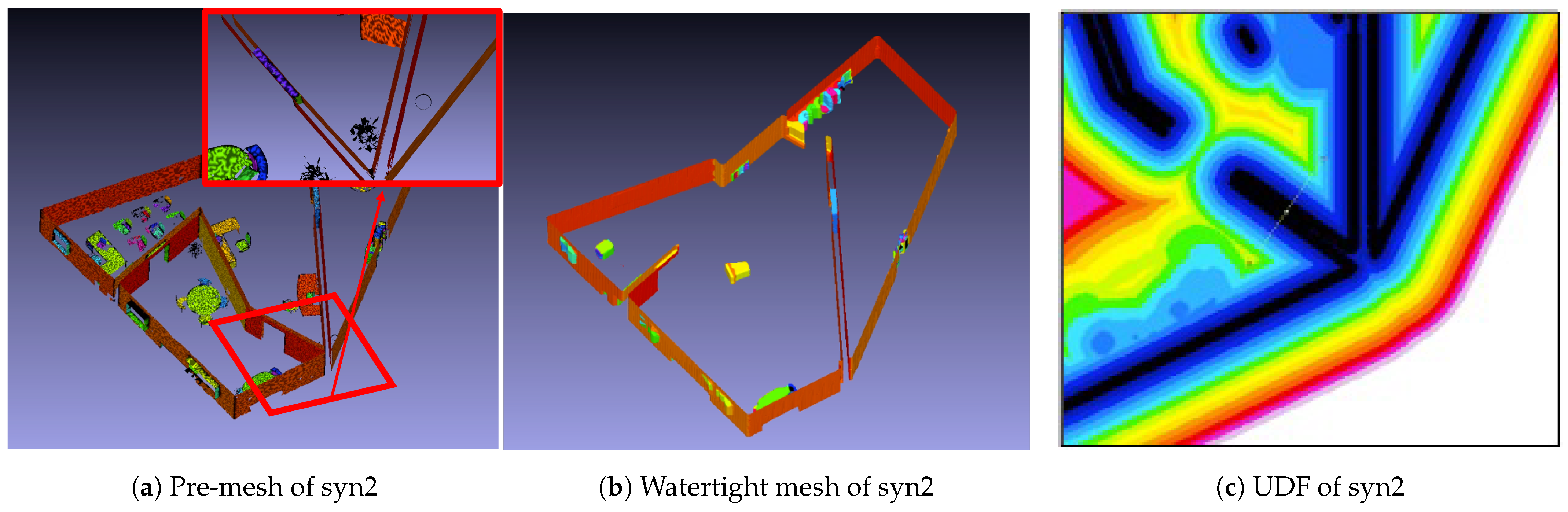
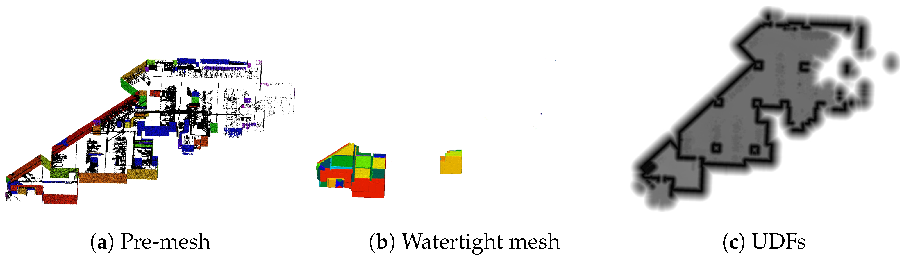
- The unsigned distance field (UDF) of the entire model is calculated (see Section 3.2.1 and Figure 4a)The UDFs of the plane meshes are then calculated. Subsequently, all UDFs are compared, and the minimum value is assigned as the distance value to generate the UDF for the entire model.
- Step 2:
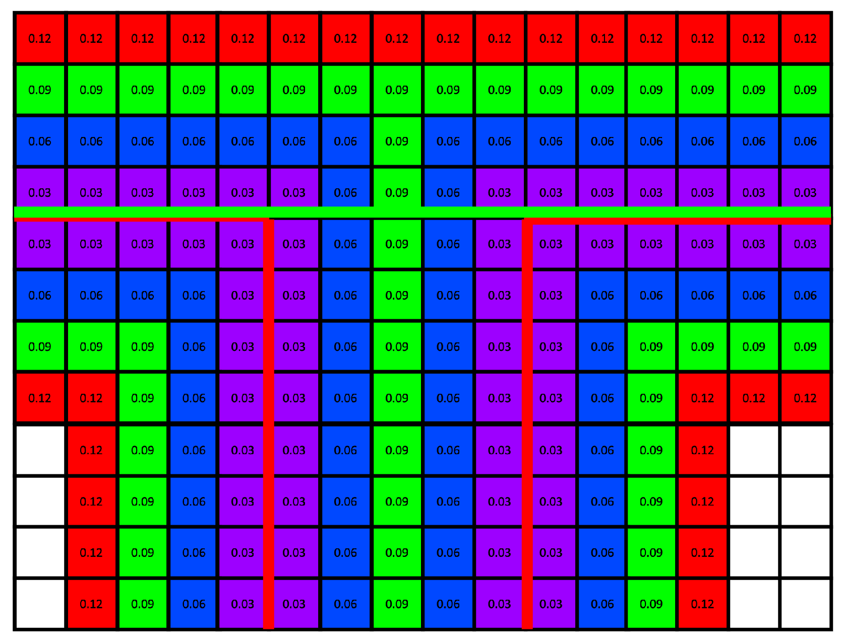
- The inside and outside of the structural model are classified (see Section 3.2.2 and Figure 4b)Using the UDF of the entire model, a surface confidence map (voxel data) labeled with , , and is generated. A subgraph is then constructed based on , and data distinguishing the interior and exterior regions of the indoor model are obtained by applying a graph-cut algorithm.
- Step 3:
- The SDF is generated (see Section 3.2.2 and Figure 4c)The SDF based on the surfaces of the indoor structures is generated using the UDF of the entire model obtained in and classification data derived in .
3.2.1. UDF Generation for the Entire Model
3.2.2. Inside/Outside Classification
3.3. Generation of Structural Components
4. Results
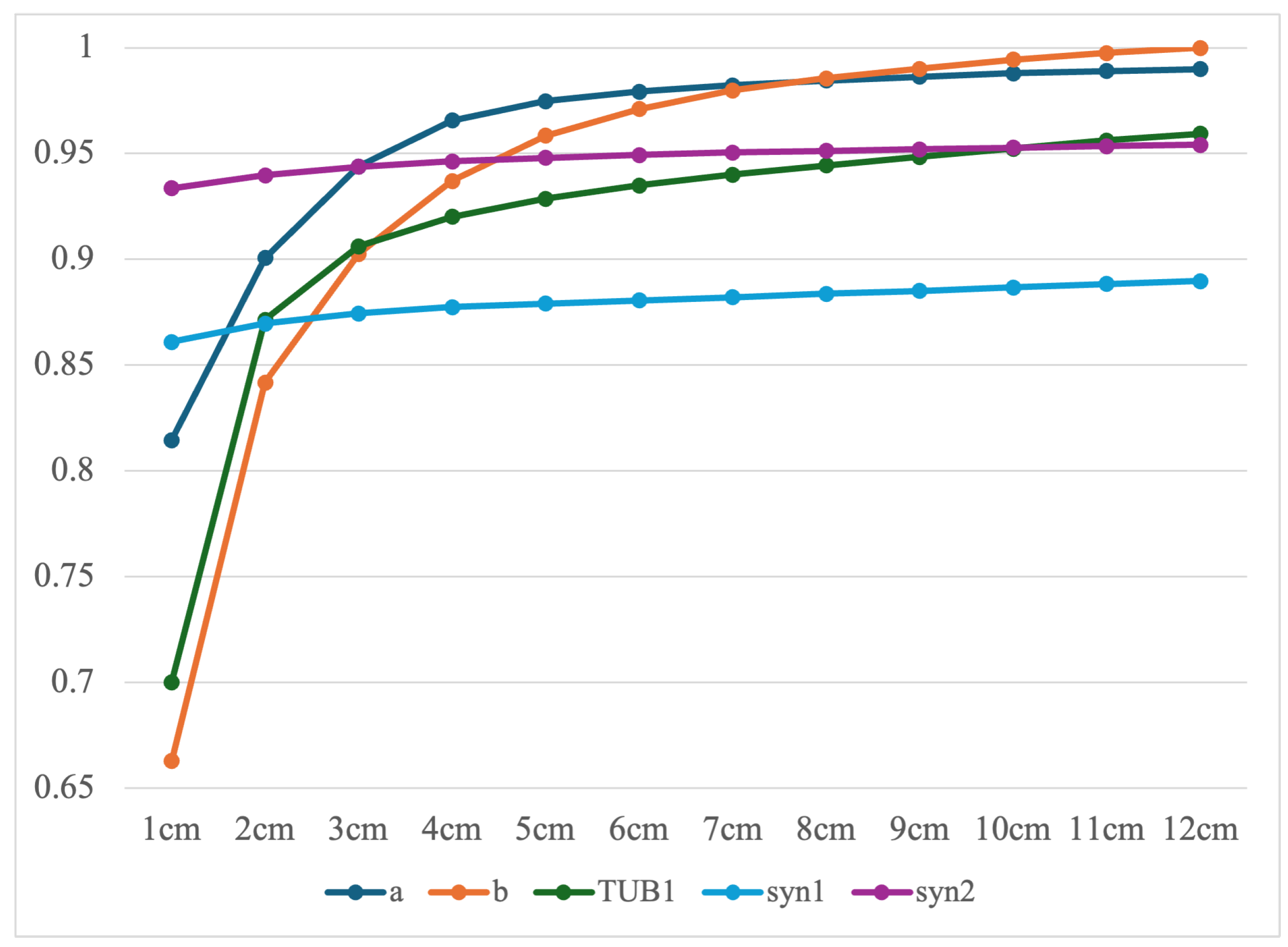
4.1. Evaluation
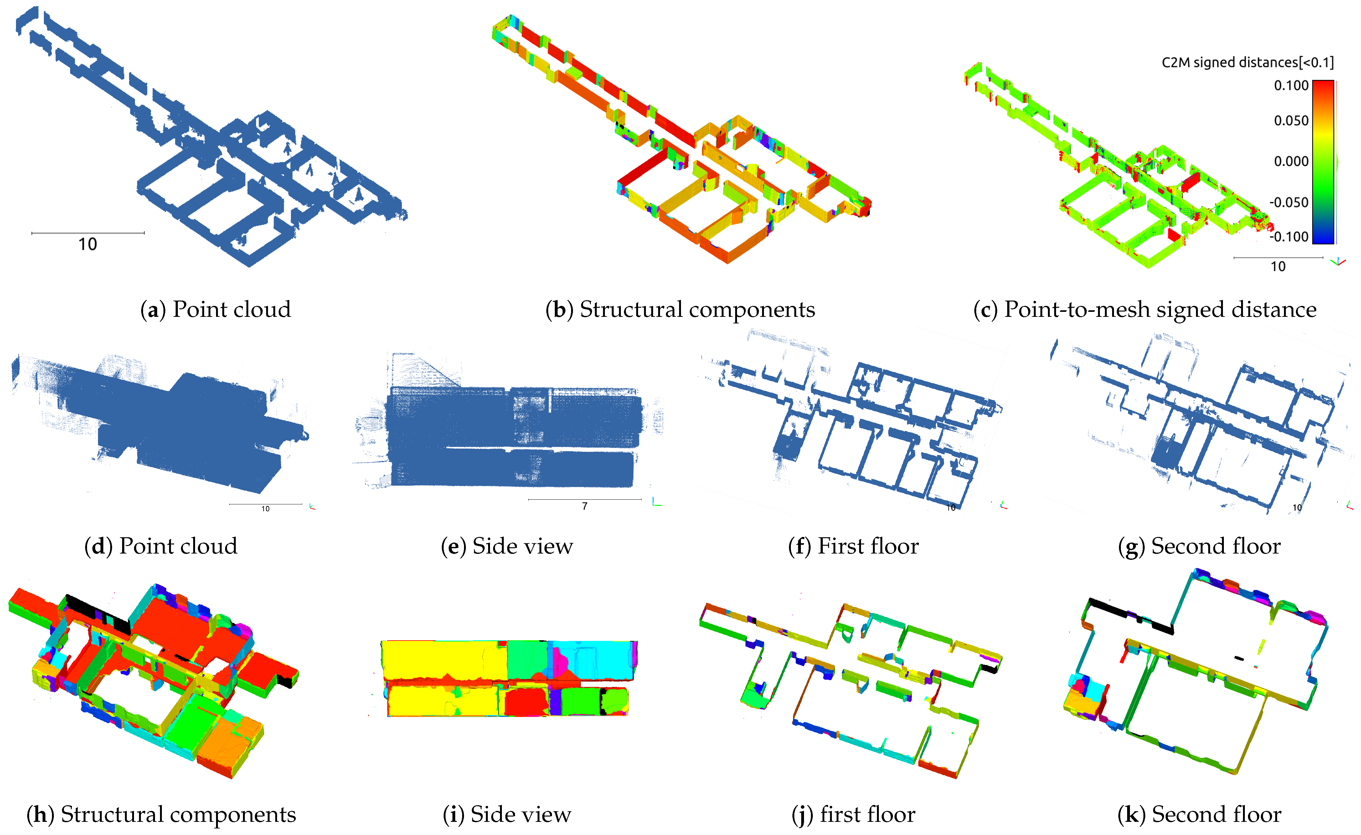
4.2. Structural Component Generation Results
4.3. Discussion
5. Conclusions
Author Contributions
Funding
Institutional Review Board Statement
Informed Consent Statement
Data Availability Statement
Conflicts of Interest
Abbreviations
| UDF | Unsigned distance function; |
| SDF | Signed distance function. |
References
- Nikoohemat, S.; Diakité, A.A.; Zlatanova, S.; Vosselman, G. Indoor 3D reconstruction from point clouds for optimal routing in complex buildings to support disaster management. Autom. Constr. 2020, 113, 103109. [Google Scholar] [CrossRef]
- Li, N.; Becerik-Gerber, B.; Krishnamachari, B.; Soibelman, L. A BIM centered indoor localization algorithm to support building fire emergency response operations. Autom. Constr. 2014, 42, 78–89. [Google Scholar] [CrossRef]
- Chen, C.; Tang, L. BIM-based integrated management workflow design for schedule and cost planning of building fabric maintenance. Autom. Constr. 2019, 107, 102944. [Google Scholar] [CrossRef]
- Chen, H.; Zhou, X.; Feng, Z.; Cao, S.J. Application of polyhedral meshing strategy in indoor environment simulation: Model accuracy and computing time. Indoor Built Environ. 2022, 31, 719–731. [Google Scholar] [CrossRef]
- Kang, Z.; Yang, J.; Yang, Z.; Cheng, S. A Review of Techniques for 3D Reconstruction of Indoor Environments. ISPRS Int. J. Geo-Inf. 2020, 9, 330. [Google Scholar] [CrossRef]
- Abdollahi, A.; Arefi, H.; Malihi, S.; Maboudi, M. Progressive Model-Driven Approach for 3D Modeling of Indoor Spaces. Sensors 2023, 23, 5934. [Google Scholar] [CrossRef] [PubMed]
- Lim, G.; Doh, N. Automatic Reconstruction of Multi-Level Indoor Spaces from Point Cloud and Trajectory. Sensors 2021, 21, 3493. [Google Scholar] [CrossRef] [PubMed]
- Hornung, A.; Kobbelt, L. Robust reconstruction of watertight 3D models from non-uniformly sampled point clouds without normal information. In Proceedings of the Fourth Eurographics Symposium on Geometry Processing, Cagliari, Italy, 26–28 June 2006; SGP ’06. pp. 41–50. [Google Scholar]
- Pintore, G.; Mura, C.; Ganovelli, F.; Fuentes-Perez, L.; Pajarola, R.; Gobbetti, E. State-of-the-art in Automatic 3D Reconstruction of Structured Indoor Environments. Comput. Graph. Forum 2020, 39, 667–699. [Google Scholar] [CrossRef]
- Bernardini, F.; Mittleman, J.; Rushmeier, H.; Silva, C.; Taubin, G. The ball-pivoting algorithm for surface reconstruction. IEEE Trans. Vis. Comput. Graph. 1999, 5, 349–359. [Google Scholar] [CrossRef]
- Kazhdan, M.; Bolitho, M.; Hoppe, H. Poisson surface reconstruction. In Proceedings of the Fourth Eurographics Symposium on Geometry Processing, Cagliari, Italy, 26–28 June 2006; SGP ’06. pp. 61–70. [Google Scholar]
- Ohtake, Y.; Belyaev, A.; Seidel, H.P. An integrating approach to meshing scattered point data. In Proceedings of the 2005 ACM Symposium on Solid and Physical Modeling, Cambridge, MA, USA, 13–15 June 2005; SPM ’05. pp. 61–69. [Google Scholar] [CrossRef]
- Li, L.; Yang, F.; Zhu, H.; Li, D.; Li, Y.; Tang, L. An Improved RANSAC for 3D Point Cloud Plane Segmentation Based on Normal Distribution Transformation Cells. Remote Sens. 2017, 9, 433. [Google Scholar] [CrossRef]
- Yang, L.; Li, Y.; Li, X.; Meng, Z.; Luo, H. Efficient plane extraction using normal estimation and RANSAC from 3D point cloud. Comput. Stand. Interfaces 2022, 82, 103608. [Google Scholar] [CrossRef]
- Ge, X.; Zhang, J.; Xu, B.; Shu, H.; Chen, M. An Efficient Plane-Segmentation Method for Indoor Point Clouds Based on Countability of Saliency Directions. ISPRS Int. J. Geo-Inf. 2022, 11, 247. [Google Scholar] [CrossRef]
- Araújo, A.M.C.; Oliveira, M.M. A robust statistics approach for plane detection in unorganized point clouds. Pattern Recognit. 2020, 100, 107115. [Google Scholar] [CrossRef]
- Oesau, S.; Lafarge, F.; Alliez, P. Indoor scene reconstruction using feature sensitive primitive extraction and graph-cut. ISPRS J. Photogramm. Remote Sens. 2014, 90, 68–82. [Google Scholar] [CrossRef]
- Previtali, M.; Díaz-Vilariño, L.; Scaioni, M. Indoor Building Reconstruction from Occluded Point Clouds Using Graph-Cut and Ray-Tracing. Appl. Sci. 2018, 8, 1529. [Google Scholar] [CrossRef]
- Yang, F.; Zhou, G.; Su, F.; Zuo, X.; Tang, L.; Liang, Y.; Zhu, H.; Li, L. Automatic Indoor Reconstruction from Point Clouds in Multi-room Environments with Curved Walls. Sensors 2019, 19, 3798. [Google Scholar] [CrossRef] [PubMed]
- Hübner, P.; Weinmann, M.; Wursthorn, S.; Hinz, S. Automatic voxel-based 3D indoor reconstruction and room partitioning from triangle meshes. ISPRS J. Photogramm. Remote Sens. 2021, 181, 254–278. [Google Scholar] [CrossRef]
- Hornung, A.; Kobbelt, L. Hierarchical Volumetric Multi-view Stereo Reconstruction of Manifold Surfaces based on Dual Graph Embedding. In Proceedings of the 2006 IEEE Computer Society Conference on Computer Vision and Pattern Recognition (CVPR’06), New York, NY, USA, 17–22 June 2006; Volume 1, pp. 503–510, ISSN 063-6919. [Google Scholar] [CrossRef]
- Ju, T.; Losasso, F.; Schaefer, S.; Warren, J. Dual contouring of hermite data. In Proceedings of the 29th Annual Conference on Computer Graphics and Interactive Techniques, SIGGRAPH ’02. San Antonio, TX, USA, 23–26 July 2002; Volume 1, pp. 339–346. [Google Scholar] [CrossRef]
- Khoshelham, K.; Díaz Vilariño, L.; Peter, M.; Kang, Z.; Acharya, D. The ISPRS Benchmark on Indoor Modelling. Int. Arch. Photogramm. Remote Sens. Spat. Inf. Sci. 2017, XLII-2-W7, 367–372. [Google Scholar] [CrossRef]
- Visualization and MultiMedia Lab, University of Zurich. VMML Research Datasets. 2024. Available online: https://www.ifi.uzh.ch/en/vmml/research/datasets.html (accessed on 2 May 2025).
- CloudCompare (Version 2.11.3) [GPL Software]. (2025). Available online: http://www.cloudcompare.org/ (accessed on 2 May 2025).
- Saroglou, T.; Meir, I.A.; Theodosiou, T.; Givoni, B. Towards energy efficient skyscrapers. Energy Build. 2017, 149, 437–449. [Google Scholar] [CrossRef]


| Datasets | Scanner | Rooms | Floors | Manhattan Assumption |
|---|---|---|---|---|
| A | BLK360 | 1 | 1 | ◯ |
| B | BLK360 | 1 | 1 | ◯ |
| TUB1 | Viametris iMS3D | 10 | 1 | ◯ |
| TUB2 | Zeb-Revo | 14 | 2 | ◯ |
| syn1 | Synthesized | 3 | 1 | △ |
| syn2 | Synthesized | 7 | 1 | × |
| Datasets | Voxel Pitch (m) | Volume Size |
|---|---|---|
| A | 0.05 | 178 × 119 × 101 |
| B | 0.05 | 211 × 212 × 108 |
| TUB1 | 0.03 | 639 × 1532 × 216 |
| TUB2 | 0.04 | 1147 × 660 × 310 |
| syn1 | 0.03 | 380 × 601 × 216 |
| syn2 | 0.03 | 862 × 852 × 249 |
| A | B | TUB1 | TUB2 | syn1 | syn2 | |||||||
|---|---|---|---|---|---|---|---|---|---|---|---|---|
| Watertight Mesh (mm) | 7.6 | 34.7 | 5.6 | 41.6 | −13.1 | 87.7 | −76.1 | 545.1 | 61.4 | 197.4 | −36.2 | 182.0 |
| Structural Components (mm) | 3.9 | 29.9 | 2.7 | 37.8 | −10.5 | 84.7 | 0 | 0 | 52.7 | 195.6 | −27.2 | 183.9 |
Disclaimer/Publisher’s Note: The statements, opinions and data contained in all publications are solely those of the individual author(s) and contributor(s) and not of MDPI and/or the editor(s). MDPI and/or the editor(s) disclaim responsibility for any injury to people or property resulting from any ideas, methods, instructions or products referred to in the content. |
© 2025 by the authors. Licensee MDPI, Basel, Switzerland. This article is an open access article distributed under the terms and conditions of the Creative Commons Attribution (CC BY) license (https://creativecommons.org/licenses/by/4.0/).
Share and Cite
Lee, J.; Ohtake, Y.; Nakano, T.; Sato, D. Generation of Structural Components for Indoor Spaces from Point Clouds. Sensors 2025, 25, 3012. https://doi.org/10.3390/s25103012
Lee J, Ohtake Y, Nakano T, Sato D. Generation of Structural Components for Indoor Spaces from Point Clouds. Sensors. 2025; 25(10):3012. https://doi.org/10.3390/s25103012
Chicago/Turabian StyleLee, Junhyuk, Yutaka Ohtake, Takashi Nakano, and Daisuke Sato. 2025. "Generation of Structural Components for Indoor Spaces from Point Clouds" Sensors 25, no. 10: 3012. https://doi.org/10.3390/s25103012
APA StyleLee, J., Ohtake, Y., Nakano, T., & Sato, D. (2025). Generation of Structural Components for Indoor Spaces from Point Clouds. Sensors, 25(10), 3012. https://doi.org/10.3390/s25103012