
Leveraging Segment Anything Model (SAM) for Weld Defect Detection in Industrial Ultrasonic B-Scan Images


Abstract
1. Introduction
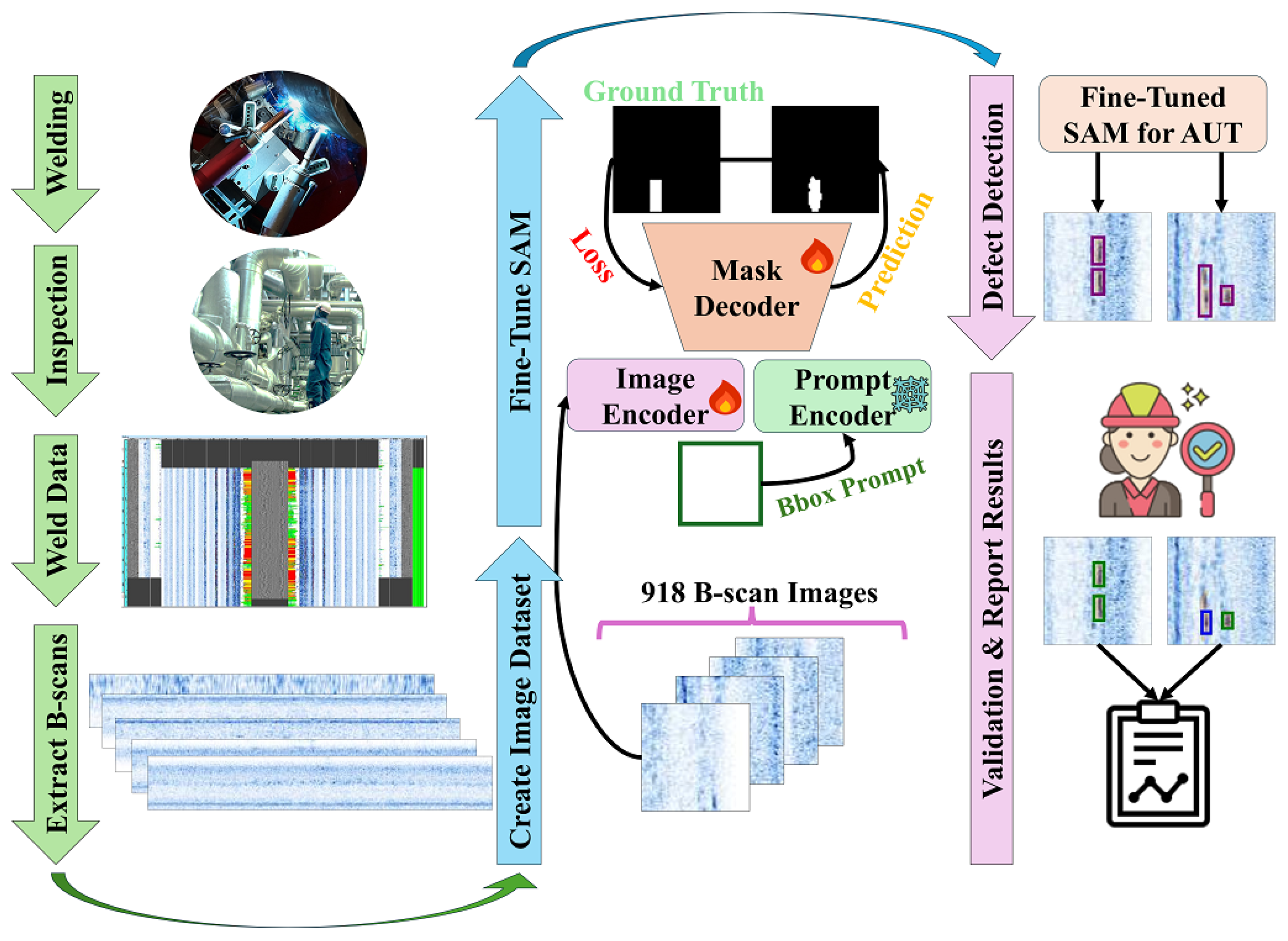
- This paper proposes a fully automated and promptable defect detection approach using SAM 1 and SAM 2, while minimizing post-processing steps and parameters compared to existing deep learning-based methods (e.g., tuning confidence thresholds, applying non-maximum suppression (NMS), etc.).
- It investigates the effects of different fine-tuning methods (vanilla and low-rank adaptation (LoRA)), various scales of training data (to address limited data scenarios), and the impact of combining loss functions (Dice loss and cross-entropy).
2. Method
2.1. Overview
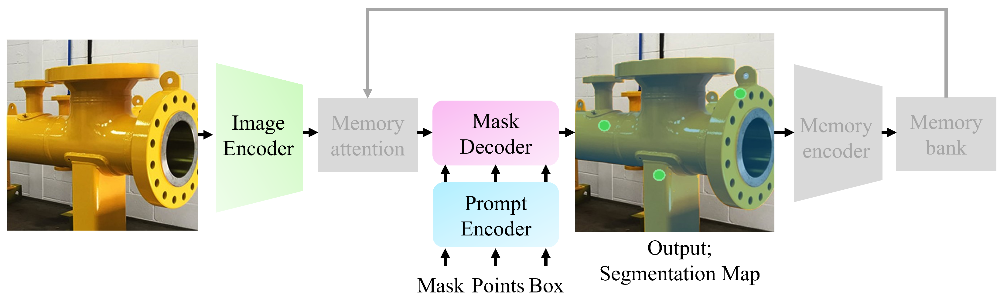
2.2. Architecture
2.2.1. Image Encoder
2.2.2. Prompt Encoder and Mask Decoder
2.2.3. Memory Attention, Memory Encoder, and Memory Bank
2.3. Vanilla and Parameter-Efficient Fine-Tuning
3. Experiments
3.1. Dataset
3.2. Environment
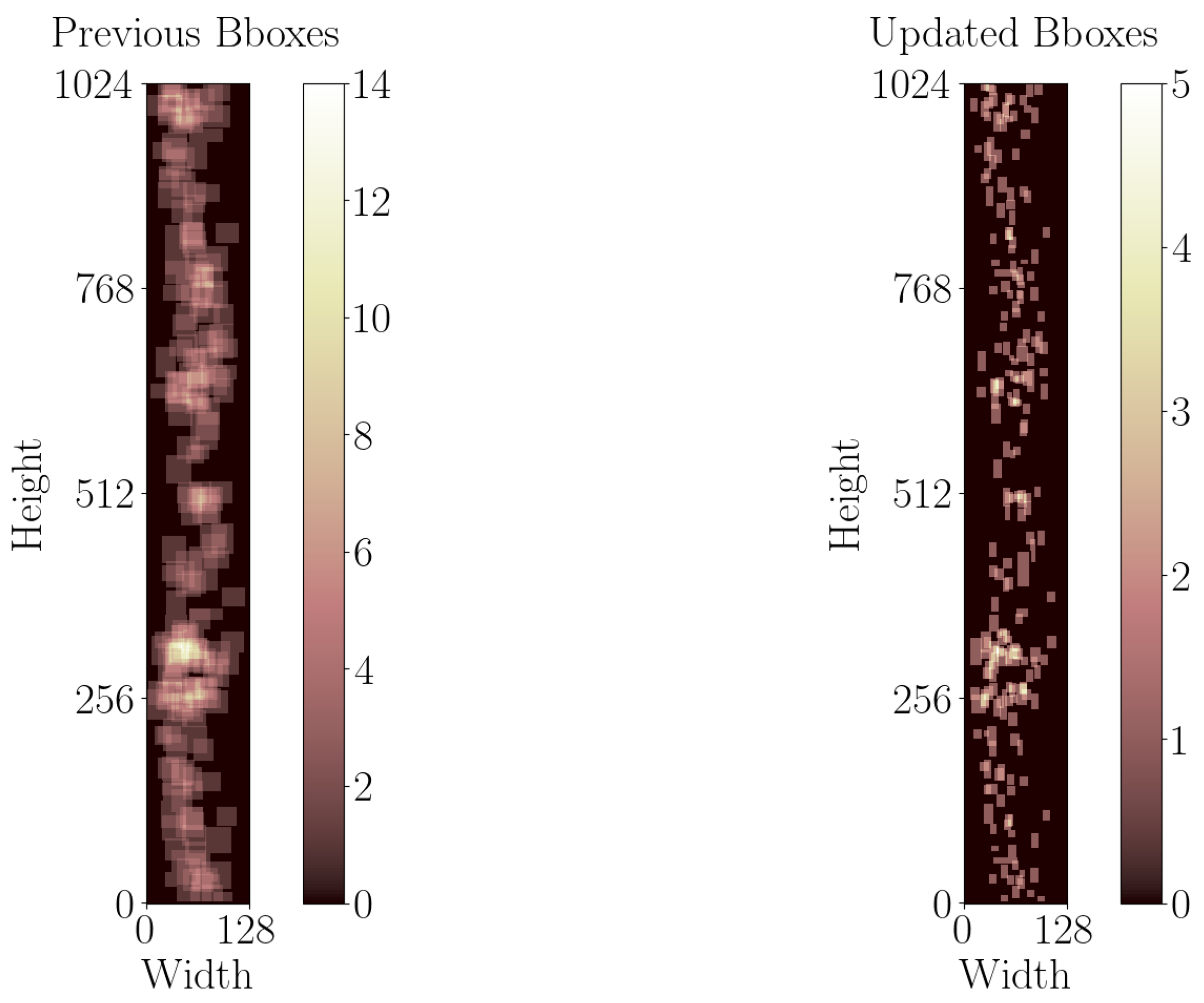
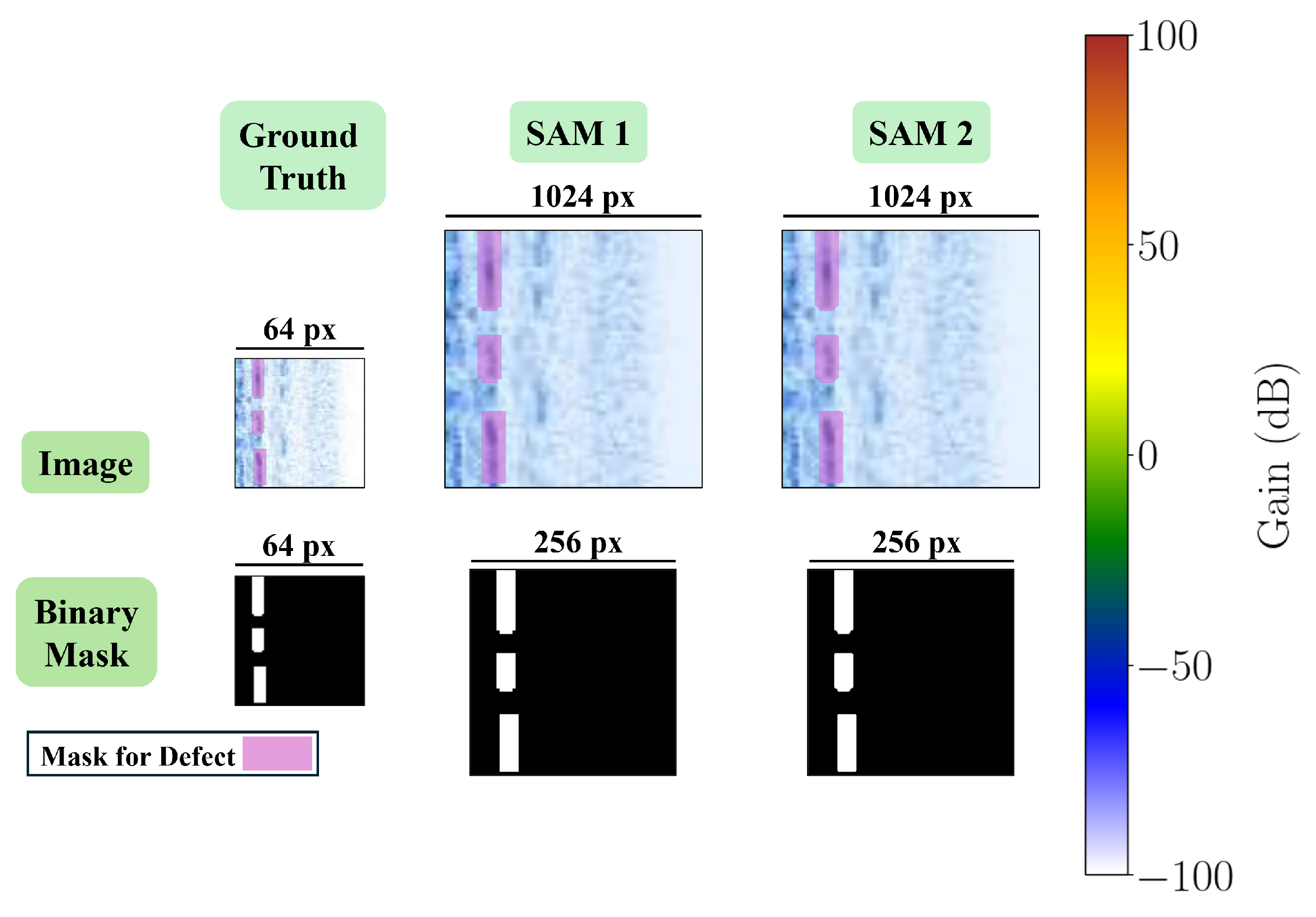
3.3. Input Data Pipeline
3.4. Evaluation Metrics
3.5. Fine-Tuning
3.5.1. Loss Function
3.5.2. LoRA Settings
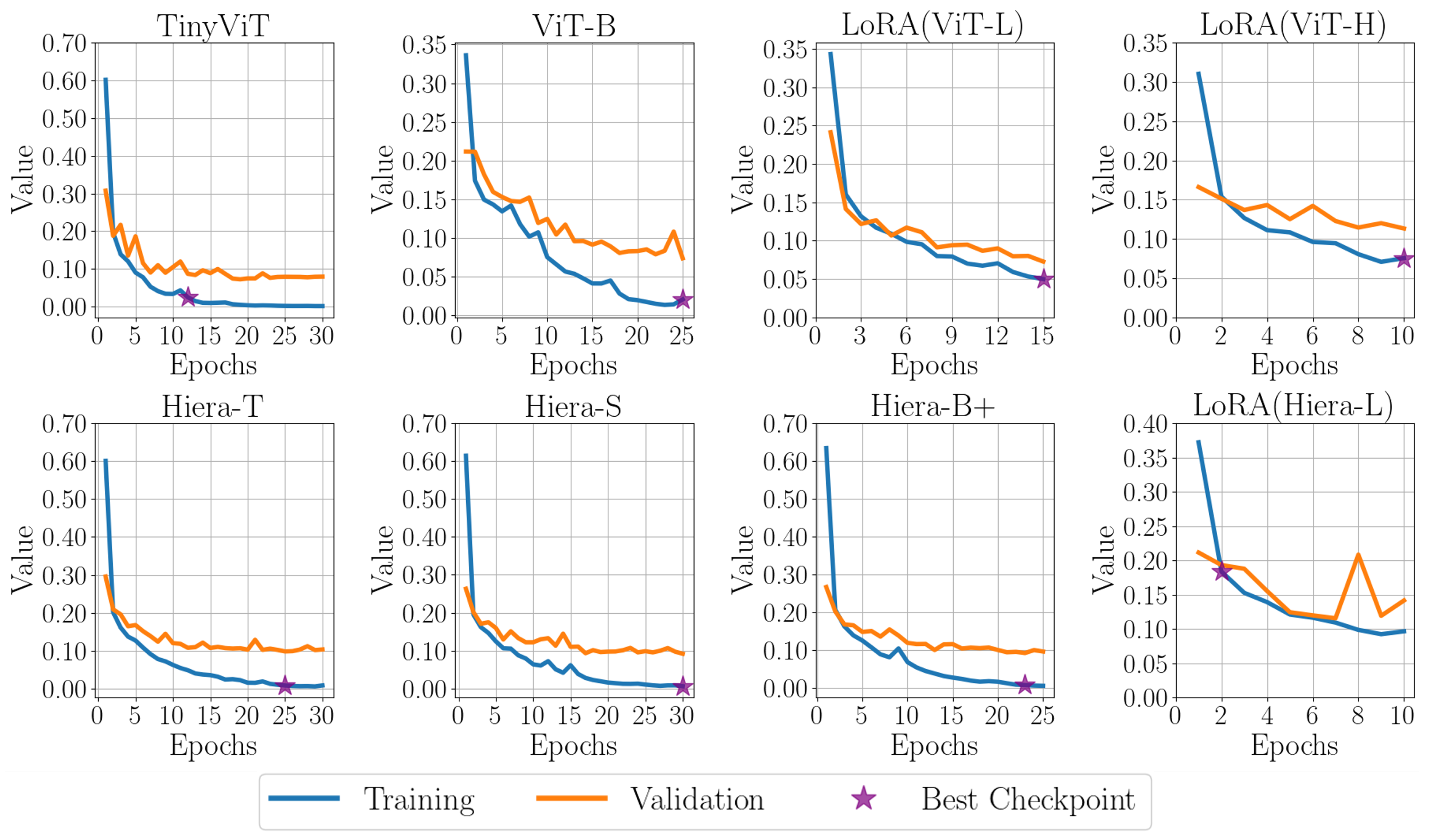
3.5.3. Fine-Tuning Overview
4. Results and Discussion
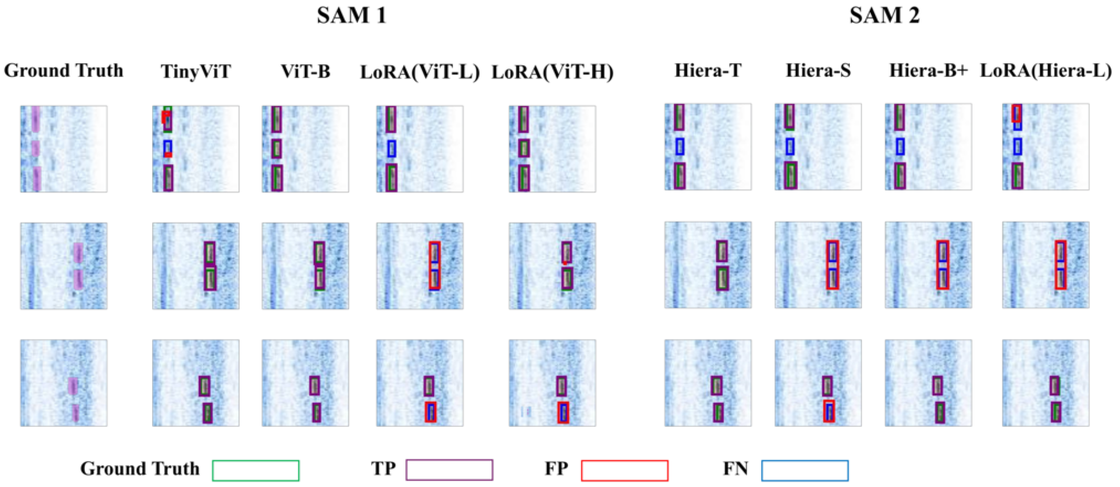
4.1. Performance Evaluation
4.2. Ablation Study
4.2.1. Why Not Just Fine-Tune the Mask Decoder?
4.2.2. Training Data Size vs. Performance
4.2.3. Cross-Entropy Loss Analysis
4.3. Limitations and Future Works
5. Conclusions
Author Contributions
Funding
Institutional Review Board Statement
Informed Consent Statement
Data Availability Statement
Conflicts of Interest
References
- LeCun, Y.; Bengio, Y.; Hinton, G. Deep learning. Nature 2015, 521, 436–444. [Google Scholar] [CrossRef] [PubMed]
- Ajmi, C.; Zapata, J.; Elferchichi, S.; Laabidi, K. Advanced Faster-RCNN Model for Automated Recognition and Detection of Weld Defects on Limited X-Ray Image Dataset. J. Nondestruct. Eval. 2024, 43, 14. [Google Scholar] [CrossRef]
- Totino, B.; Spagnolo, F.; Perri, S. RIAWELC: A Novel dataset of radiographic images for automatic weld defects classification. Int. J. Electr. Comput. Eng. Res. 2023, 3, 13–17. [Google Scholar] [CrossRef]
- Naddaf-Sh, S.; Naddaf-Sh, M.M.; Zargarzadeh, H.; Dalton, M.; Ramezani, S.; Elpers, G.; Baburao, V.S.; Kashani, A.R. Real-Time Explainable Multiclass Object Detection for Quality Assessment in 2-Dimensional Radiography Images. Complexity 2022, 2022, 4637939. [Google Scholar] [CrossRef]
- Naddaf-Sh, M.M.; Naddaf-Sh, S.; Zargarzadeh, H.; Zahiri, S.M.; Dalton, M.; Elpers, G.; Kashani, A.R. 9—Defect detection and classification in welding using deep learning and digital radiography. In Fault Diagnosis and Prognosis Techniques for Complex Engineering Systems; Karimi, H., Ed.; Academic Press: Cambridge, MA, USA, 2021; pp. 327–352. [Google Scholar] [CrossRef]
- Kim, Y.H.; Lee, J.R. Automated data evaluation in phased-array ultrasonic testing based on A-scan and feature training. NDT E Int. 2024, 141, 102974. [Google Scholar] [CrossRef]
- Pyle, R.J.; Bevan, R.L.; Hughes, R.R.; Rachev, R.K.; Ali, A.A.S.; Wilcox, P.D. Deep learning for ultrasonic crack characterization in NDE. IEEE Trans. Ultrason. Ferroelectr. Freq. Control 2020, 68, 1854–1865. [Google Scholar] [CrossRef]
- Medak, D.; Posilović, L.; Subašić, M.; Budimir, M.; Lončarić, S. Automated defect detection from ultrasonic images using deep learning. IEEE Trans. Ultrason. Ferroelectr. Freq. Control 2021, 68, 3126–3134. [Google Scholar] [CrossRef]
- Ye, J.; Ito, S.; Toyama, N. Computerized ultrasonic imaging inspection: From shallow to deep learning. Sensors 2018, 18, 3820. [Google Scholar] [CrossRef]
- Block, S.B.; Da Silva, R.D.; Lazzaretti, A.E.; Minetto, R. LoHi-WELD: A novel industrial dataset for weld defect detection and classification, a deep learning study, and future perspectives. IEEE Access 2024, 12, 77442–77453. [Google Scholar] [CrossRef]
- Qi, H.; Cheng, L.; Kong, X.; Zhang, J.; Gu, J. WDLS: Deep Level Set Learning for Weakly Supervised Aeroengine Defect Segmentation. IEEE Trans. Ind. Inform. 2024, 20, 303–313. [Google Scholar] [CrossRef]
- Tu, X.L.; Zhang, J.; Gambaruto, A.M.; Wilcox, P.D. A framework for computing directivities for ultrasonic sources in generally anisotropic, multi-layered media. Wave Motion 2024, 128, 103299. [Google Scholar] [CrossRef]
- Swornowski, P.J. Scanning of the internal structure part with laser ultrasonic in aviation industry. Scanning 2011, 33, 378–385. [Google Scholar] [CrossRef] [PubMed]
- Dwivedi, S.K.; Vishwakarma, M.; Soni, A. Advances and researches on non destructive testing: A review. Mater. Today Proc. 2018, 5, 3690–3698. [Google Scholar] [CrossRef]
- Cantero-Chinchilla, S.; Croxford, A.J.; Wilcox, P.D. Optimising laser-induced phased-arrays for defect detection in continuous inspections. NDT E Int. 2024, 144, 103091. [Google Scholar] [CrossRef]
- Xie, L.; Lian, Y.; Du, F.; Wang, Y.; Lu, Z. Optical methods of laser ultrasonic testing technology in the industrial and engineering applications: A review. Opt. Laser Technol. 2024, 176, 110876. [Google Scholar] [CrossRef]
- Davis, G.; Stratoudaki, T.; Lukacs, P.; Riding, M.W.; Al Fuwaires, A.; Kamintzis, P.; Pieris, D.; Keenan, A.; Wilcox, P.; Pierce, G.; et al. Near-surface defect detection in additively manufactured components using laser induced phased arrays with surface acoustic wave crosstalk suppression. Mater. Des. 2023, 236, 112453. [Google Scholar] [CrossRef]
- Krizhevsky, A.; Sutskever, I.; Hinton, G.E. ImageNet Classification with Deep Convolutional Neural Networks. In Proceedings of the Advances in Neural Information Processing Systems; Pereira, F., Burges, C., Bottou, L., Weinberger, K., Eds.; Curran Associates, Inc.: Newry, UK,, 2012; Volume 25. [Google Scholar]
- Posilović, L.; Medak, D.; Subašić, M.; Petković, T.; Budimir, M.; Lončarić, S. Flaw Detection from Ultrasonic Images using YOLO and SSD. In Proceedings of the 2019 11th International Symposium on Image and Signal Processing and Analysis (ISPA), Dubrovnik, Croatia, 23–25 September 2019; pp. 163–168. [Google Scholar] [CrossRef]
- Medak, D.; Posilović, L.; Subašić, M.; Budimir, M.; Lončarić, S. DefectDet: A deep learning architecture for detection of defects with extreme aspect ratios in ultrasonic images. Neurocomputing 2022, 473, 107–115. [Google Scholar] [CrossRef]
- Tan, M.; Pang, R.; Le, Q.V. EfficientDet: Scalable and Efficient Object Detection. arXiv 2020, arXiv:1911.09070. [Google Scholar] [CrossRef]
- Virkkunen, I.; Koskinen, T.; Jessen-Juhler, O.; Rinta-Aho, J. Augmented ultrasonic data for machine learning. J. Nondestruct. Eval. 2021, 40, 4. [Google Scholar] [CrossRef]
- Goodfellow, I.; Pouget-Abadie, J.; Mirza, M.; Xu, B.; Warde-Farley, D.; Ozair, S.; Courville, A.; Bengio, Y. Generative adversarial nets. Adv. Neural Inf. Process. Syst. 2014, 27, 2672–2680. [Google Scholar]
- Posilović, L.; Medak, D.; Subašić, M.; Budimir, M.; Lončarić, S. Generative adversarial network with object detector discriminator for enhanced defect detection on ultrasonic B-scans. Neurocomputing 2021, 459, 361–369. [Google Scholar] [CrossRef]
- Posilović, L.; Medak, D.; Subašić, M.; Budimir, M.; Lončarić, S. Generating ultrasonic images indistinguishable from real images using Generative Adversarial Networks. Ultrasonics 2022, 119, 106610. [Google Scholar] [CrossRef] [PubMed]
- Posilović, L.; Medak, D.; Milković, F.; Subašić, M.; Budimir, M.; Lončarić, S. Deep learning-based anomaly detection from ultrasonic images. Ultrasonics 2022, 124, 106737. [Google Scholar] [CrossRef] [PubMed]
- Akcay, S.; Atapour-Abarghouei, A.; Breckon, T.P. GANomaly: Semi-Supervised Anomaly Detection via Adversarial Training. arXiv 2018, arXiv:1805.06725. [Google Scholar] [CrossRef]
- Defard, T.; Setkov, A.; Loesch, A.; Audigier, R. PaDiM: A Patch Distribution Modeling Framework for Anomaly Detection and Localization. arXiv 2020, arXiv:2011.08785. [Google Scholar] [CrossRef]
- Rudolph, M.; Wandt, B.; Rosenhahn, B. Same Same However, DifferNet: Semi-Supervised Defect Detection with Normalizing Flows. arXiv 2020, arXiv:2008.12577. [Google Scholar] [CrossRef]
- Milković, F.; Filipović, B.; Subašić, M.; Petković, T.; Lončarić, S.; Budimir, M. Ultrasound Anomaly Detection Based on Variational Autoencoders. In Proceedings of the 2021 12th International Symposium on Image and Signal Processing and Analysis (ISPA), Zagreb, Croatia, 13–15 September 2021; pp. 225–229. [Google Scholar] [CrossRef]
- Kingma, D.P. Auto-encoding variational bayes. arXiv 2013, arXiv:1312.6114. [Google Scholar]
- Shi, X.; Chen, Z.; Wang, H.; Yeung, D.Y.; Wong, W.K.; Woo, W.c. Convolutional LSTM network: A machine learning approach for precipitation nowcasting. Adv. Neural Inf. Process. Syst. 2015, 28, 802–810. [Google Scholar]
- Medak, D.; Posilović, L.; Subašić, M.; Budimir, M.; Lončarić, S. Deep Learning-Based Defect Detection From Sequences of Ultrasonic B-Scans. IEEE Sens. J. 2022, 22, 2456–2463. [Google Scholar] [CrossRef]
- Ye, J.; Toyama, N. Automatic defect detection for ultrasonic wave propagation imaging method using spatio-temporal convolution neural networks. Struct. Health Monit. 2022, 21, 2750–2767. [Google Scholar] [CrossRef]
- Naddaf-Sh, A.M.; Baburao, V.S.; Zargarzadeh, H. Automated Weld Defect Detection in Industrial Ultrasonic B-Scan Images Using Deep Learning. NDT 2024, 2, 108–127. [Google Scholar] [CrossRef]
- Zhu, X.; Su, W.; Lu, L.; Li, B.; Wang, X.; Dai, J. Deformable detr: Deformable transformers for end-to-end object detection. arXiv 2020, arXiv:2010.04159. [Google Scholar]
- Jocher, G.; Chaurasia, A.; Qiu, J. Ultralytics YOLOv8. J. Comput. Commun. 2023, 11. Available online: https://github.com/ultralytics/ultralytics (accessed on 27 November 2023).
- Bommasani, R.; Hudson, D.A.; Adeli, E.; Altman, R.; Arora, S.; von Arx, S.; Bernstein, M.S.; Bohg, J.; Bosselut, A.; Brunskill, E.; et al. On the opportunities and risks of foundation models. arXiv 2021, arXiv:2108.07258. [Google Scholar]
- Achiam, J.; Adler, S.; Agarwal, S.; Ahmad, L.; Akkaya, I.; Aleman, F.L.; Almeida, D.; Altenschmidt, J.; Altman, S.; Anadkat, S.; et al. Gpt-4 technical report. arXiv 2023, arXiv:2303.08774. [Google Scholar]
- Dubey, A.; Jauhri, A.; Pandey, A.; Kadian, A.; Al-Dahle, A.; Letman, A.; Mathur, A.; Schelten, A.; Yang, A.; Fan, A.; et al. The llama 3 herd of models. arXiv 2024, arXiv:2407.21783. [Google Scholar]
- Reid, M.; Savinov, N.; Teplyashin, D.; Lepikhin, D.; Lillicrap, T.; Alayrac, J.b.; Soricut, R.; Lazaridou, A.; Firat, O.; Schrittwieser, J.; et al. Gemini 1.5: Unlocking multimodal understanding across millions of tokens of context. arXiv 2024, arXiv:2403.05530. [Google Scholar]
- Ramesh, A.; Pavlov, M.; Goh, G.; Gray, S.; Voss, C.; Radford, A.; Chen, M.; Sutskever, I. Zero-shot text-to-image generation. In Proceedings of the International Conference on Machine Learning. PMLR, Online, 18–24 July 2021; pp. 8821–8831. [Google Scholar]
- Wang, X.; Zhang, X.; Cao, Y.; Wang, W.; Shen, C.; Huang, T. Seggpt: Segmenting everything in context. arXiv 2023, arXiv:2304.03284. [Google Scholar]
- Kirillov, A.; Mintun, E.; Ravi, N.; Mao, H.; Rolland, C.; Gustafson, L.; Xiao, T.; Whitehead, S.; Berg, A.C.; Lo, W.Y.; et al. Segment anything. In Proceedings of the IEEE/CVF International Conference on Computer Vision, Paris, France, 1–6 October 2023; pp. 4015–4026. [Google Scholar]
- Ravi, N.; Gabeur, V.; Hu, Y.T.; Hu, R.; Ryali, C.; Ma, T.; Khedr, H.; Rädle, R.; Rolland, C.; Gustafson, L.; et al. Sam 2: Segment anything in images and videos. arXiv 2024, arXiv:2408.00714. [Google Scholar]
- Ma, J.; He, Y.; Li, F.; Han, L.; You, C.; Wang, B. Segment anything in medical images. Nat. Commun. 2024, 15, 654. [Google Scholar] [CrossRef]
- Mou, L.; Zhao, Y.; Fu, H.; Liu, Y.; Cheng, J.; Zheng, Y.; Su, P.; Yang, J.; Chen, L.; Frangi, A.F.; et al. Segment Anything Model for Medical Images? Med. Image Anal. 2023, 92, 103061. [Google Scholar]
- Deng, R.; Cui, C.; Liu, Q.; Yao, T.; Remedios, L.W.; Bao, S.; Landman, B.A.; Wheless, L.E.; Coburn, L.A.; Wilson, K.T.; et al. Segment Anything Model (SAM) for Digital Pathology: Assess Zero-shot Segmentation on Whole Slide Imaging. arXiv 2023, arXiv:2304.04155. [Google Scholar]
- Zhang, Y.; Shen, Z.; Jiao, R. Segment anything model for medical image segmentation: Current applications and future directions. Comput. Biol. Med. 2024, 171, 108238. [Google Scholar] [CrossRef] [PubMed]
- Osco, L.P.; Wu, Q.; de Lemos, E.L.; Gonçalves, W.N.; Ramos, A.P.M.; Li, J.; Marcato, J. The Segment Anything Model (SAM) for remote sensing applications: From zero to one shot. Int. J. Appl. Earth Obs. Geoinf. 2023, 124, 103540. [Google Scholar] [CrossRef]
- Cao, Y.; Xu, X.; Sun, C.; Cheng, Y.; Du, Z.; Gao, L.; Shen, W. Segment any anomaly without training via hybrid prompt regularization. arXiv 2023, arXiv:2305.10724. [Google Scholar]
- Hu, B.; Gao, B.; Tan, C.; Wu, T.; Li, S.Z. Segment anything in defect detection. arXiv 2023, arXiv:2311.10245. [Google Scholar]
- Ahmadi, M.; Lonbar, A.G.; Sharifi, A.; Beris, A.T.; Nouri, M.; Javidi, A.S. Application of segment anything model for civil infrastructure defect assessment. arXiv 2023, arXiv:2304.12600. [Google Scholar]
- Ding, H.; Gao, J.; Yuan, Y.; Wang, Q. SamLP: A Customized Segment Anything Model for License Plate Detection. arXiv 2024, arXiv:2401.06374. [Google Scholar]
- Dosovitskiy, A. An image is worth 16×16 words: Transformers for image recognition at scale. arXiv 2020, arXiv:2010.11929. [Google Scholar]
- Wu, K.; Zhang, J.; Peng, H.; Liu, M.; Xiao, B.; Fu, J.; Yuan, L. Tinyvit: Fast pretraining distillation for small vision transformers. In Proceedings of the European Conference on Computer Vision, Tel Aviv, Israel, 23–27 October 2022; Springer: Cham, Switzerland, 2022; pp. 68–85. [Google Scholar]
- He, K.; Chen, X.; Xie, S.; Li, Y.; Dollár, P.; Girshick, R. Masked autoencoders are scalable vision learners. In Proceedings of the IEEE/CVF Conference on Computer Vision and Pattern Recognition, New Orleans, LA, USA, 18–24 June 2022; pp. 16000–16009. [Google Scholar]
- Li, Y.; Mao, H.; Girshick, R.; He, K. Exploring plain vision transformer backbones for object detection. In Proceedings of the European Conference on Computer Vision, Tel Aviv, Israel, 23–27 October 2022; Springer: Cham, Switzerland, 2022; pp. 280–296. [Google Scholar]
- Vaswani, A. Attention is all you need. Adv. Neural Inf. Process. Syst. 2017, 30, 5998–6008. [Google Scholar]
- Ba, J.L. Layer normalization. arXiv 2016, arXiv:1607.06450. [Google Scholar]
- Zhang, C.; Han, D.; Qiao, Y.; Kim, J.U.; Bae, S.H.; Lee, S.; Hong, C.S. Faster Segment Anything: Towards Lightweight SAM for Mobile Applications. arXiv 2023, arXiv:2306.14289. [Google Scholar]
- Howard, A.; Sandler, M.; Chu, G.; Chen, L.C.; Chen, B.; Tan, M.; Wang, W.; Zhu, Y.; Pang, R.; Vasudevan, V.; et al. Searching for mobilenetv3. In Proceedings of the IEEE/CVF International Conference on Computer Vision, Seoul, Republic of Korea, 27 October–2 November 2019; pp. 1314–1324. [Google Scholar]
- Hendrycks, D.; Gimpel, K. Gaussian error linear units (gelus). arXiv 2016, arXiv:1606.08415. [Google Scholar]
- Ioffe, S. Batch normalization: Accelerating deep network training by reducing internal covariate shift. arXiv 2015, arXiv:1502.03167. [Google Scholar]
- Ryali, C.; Hu, Y.T.; Bolya, D.; Wei, C.; Fan, H.; Huang, P.Y.; Aggarwal, V.; Chowdhury, A.; Poursaeed, O.; Hoffman, J.; et al. Hiera: A hierarchical vision transformer without the bells-and-whistles. In Proceedings of the International Conference on Machine Learning, PMLR, Honolulu, HI, USA, 23–29 July 2023; pp. 29441–29454. [Google Scholar]
- Li, Y.; Wu, C.Y.; Fan, H.; Mangalam, K.; Xiong, B.; Malik, J.; Feichtenhofer, C. Mvitv2: Improved multiscale vision transformers for classification and detection. In Proceedings of the IEEE/CVF Conference on COMPUTER vision and Pattern Recognition, New Orleans, LA, USA, 18–24 June 2022; pp. 4804–4814. [Google Scholar]
- Bolya, D.; Ryali, C.; Hoffman, J.; Feichtenhofer, C. Window Attention is Bugged: How not to Interpolate Position Embeddings. arXiv 2023, arXiv:2311.05613. [Google Scholar]
- Lin, T.Y.; Dollár, P.; Girshick, R.; He, K.; Hariharan, B.; Belongie, S. Feature pyramid networks for object detection. In Proceedings of the IEEE Conference on Computer Vision and Pattern Recognition, Honolulu, HI, USA, 21–26 July 2017; pp. 2117–2125. [Google Scholar]
- Radford, A.; Kim, J.W.; Hallacy, C.; Ramesh, A.; Goh, G.; Agarwal, S.; Sastry, G.; Askell, A.; Mishkin, P.; Clark, J.; et al. Learning transferable visual models from natural language supervision. In Proceedings of the International Conference on Machine Learning, PMLR, Online, 18–24 July 2021; pp. 8748–8763. [Google Scholar]
- Azizi, S.; Culp, L.; Freyberg, J.; Mustafa, B.; Baur, S.; Kornblith, S.; Chen, T.; MacWilliams, P.; Mahdavi, S.S.; Wulczyn, E.; et al. Robust and efficient medical imaging with self-supervision. arXiv 2022, arXiv:2205.09723. [Google Scholar]
- Ding, N.; Qin, Y.; Yang, G.; Wei, F.; Yang, Z.; Su, Y.; Hu, S.; Chen, Y.; Chan, C.M.; Chen, W.; et al. Parameter-efficient fine-tuning of large-scale pre-trained language models. Nat. Mach. Intell. 2023, 5, 220–235. [Google Scholar] [CrossRef]
- Dutt, R.; Ericsson, L.; Sanchez, P.; Tsaftaris, S.A.; Hospedales, T. Parameter-efficient fine-tuning for medical image analysis: The missed opportunity. arXiv 2023, arXiv:2305.08252. [Google Scholar]
- Aghajanyan, A.; Zettlemoyer, L.; Gupta, S. Intrinsic dimensionality explains the effectiveness of language model fine-tuning. arXiv 2020, arXiv:2012.13255. [Google Scholar]
- Hu, E.J.; Shen, Y.; Wallis, P.; Allen-Zhu, Z.; Li, Y.; Wang, S.; Wang, L.; Chen, W. Lora: Low-rank adaptation of large language models. arXiv 2021, arXiv:2106.09685. [Google Scholar]
- Gu, H.; Dong, H.; Yang, J.; Mazurowski, M.A. How to build the best medical image segmentation algorithm using foundation models: A comprehensive empirical study with Segment Anything Model. arXiv 2024, arXiv:2404.09957. [Google Scholar]
- Zhang, K.; Liu, D. Customized Segment Anything Model for Medical Image Segmentation. arXiv 2023, arXiv:2304.13785. [Google Scholar]
- Wada, K. Labelme: Image Polygonal Annotation with Python. Available online: https://zenodo.org/records/5711226 (accessed on 28 June 2024).
- Paszke, A.; Gross, S.; Massa, F.; Lerer, A.; Bradbury, J.; Chanan, G.; Killeen, T.; Lin, Z.; Gimelshein, N.; Antiga, L.; et al. Pytorch: An imperative style, high-performance deep learning library. Adv. Neural Inf. Process. Syst. 2019, 32, 8026–8037. [Google Scholar]
- Russakovsky, O.; Deng, J.; Su, H.; Krause, J.; Satheesh, S.; Ma, S.; Huang, Z.; Karpathy, A.; Khosla, A.; Bernstein, M.; et al. ImageNet Large Scale Visual Recognition Challenge. Int. J. Comput. Vis. (IJCV) 2015, 115, 211–252. [Google Scholar] [CrossRef]
- van der Walt, S.J.; Schönberger, J.L.; Nunez-Iglesias, J.; Boulogne, F.; Warner, J.D.; Yager, N.; Gouillart, E.; Yu, T.; the scikit-image Contributors. scikit-image: Image processing in Python. PeerJ 2014, 2, e453. [Google Scholar] [CrossRef]
- Zhang, Y.; Ni, Q. A Novel Weld-Seam Defect Detection Algorithm Based on the S-YOLO Model. Axioms 2023, 12, 697. [Google Scholar] [CrossRef]
- Milletari, F.; Navab, N.; Ahmadi, S.A. V-net: Fully convolutional neural networks for volumetric medical image segmentation. In Proceedings of the 2016 Fourth International Conference on 3D Vision (3DV), Stanford, CA, USA, 25–28 October 2016; IEEE: Piscataway, NJ, USA, 2016; pp. 565–571. [Google Scholar]
- Isensee, F.; Jaeger, P.F.; Kohl, S.A.; Petersen, J.; Maier-Hein, K.H. nnU-Net: A self-configuring method for deep learning-based biomedical image segmentation. Nat. Methods 2021, 18, 203–211. [Google Scholar] [CrossRef]
- Ma, J.; Chen, J.; Ng, M.; Huang, R.; Li, Y.; Li, C.; Yang, X.; Martel, A.L. Loss Odyssey in Medical Image Segmentation. Med. Image Anal. 2021, 71, 102035. [Google Scholar] [CrossRef]
- Cardoso, M.J.; Li, W.; Brown, R.; Ma, N.; Kerfoot, E.; Wang, Y.; Murrey, B.; Myronenko, A.; Zhao, C.; Yang, D.; et al. Monai: An open-source framework for deep learning in healthcare. arXiv 2022, arXiv:2211.02701. [Google Scholar]
- Zhu, Y.; Shen, Z.; Zhao, Z.; Wang, S.; Wang, X.; Zhao, X.; Shen, D.; Wang, Q. MeLo: Low-rank Adaptation is Better than Fine-tuning for Medical Image Diagnosis. arXiv 2023, arXiv:2311.08236. [Google Scholar] [CrossRef]
- Mangrulkar, S.; Gugger, S.; Debut, L.; Belkada, Y.; Paul, S.; Bossan, B. PEFT: State-of-the-Art Parameter-Efficient Fine-Tuning Methods. 2022. Available online: https://github.com/huggingface/peft (accessed on 1 October 2024).
- Ma, J.; Kim, S.; Li, F.; Baharoon, M.; Asakereh, R.; Lyu, H.; Wang, B. Segment anything in medical images and videos: Benchmark and deployment. arXiv 2024, arXiv:2408.03322. [Google Scholar]
- Rombach, R.; Blattmann, A.; Lorenz, D.; Esser, P.; Ommer, B. High-resolution image synthesis with latent diffusion models. In Proceedings of the IEEE/CVF Conference on Computer Vision and Pattern Recognition, New Orleans, LA, USA, 18–24 June 2022; pp. 10684–10695. [Google Scholar]
- Zhu, L.; Liao, B.; Zhang, Q.; Wang, X.; Liu, W.; Wang, X. Vision mamba: Efficient visual representation learning with bidirectional state space model. arXiv 2024, arXiv:2401.09417. [Google Scholar]


| Model | #Channels | #Blocks | #Heads | Global Attn. Blocks |
|---|---|---|---|---|
| ViT-Base | 768 | 12 | 12 | [2-5-8-11] |
| ViT-Large | 1024 | 24 | 16 | [5-11-17-23] |
| ViT-Huge | 1280 | 32 | 16 | [7-15-23-31] |
| TinyViT | [128-160-320] | [2-6-2] | [4-5-10] | — |
| Hiera-T | [96-192-384-768] | [1-2-7-2] | [1-2-4-8] | [5-7-9] |
| Hiera-S | [96-192-384-768] | [1-2-11-2] | [1-2-4-8] | [7-10-13] |
| Hiera-B+ | [112-224-448-896] | [2-3-16-3] | [2-4-8-16] | [12-16-20] |
| Hiera-L | [144-288-576-1152] | [2-6-36-4] | [2-4-8-16] | [23-33-43] |
| Split | Fold 1 | Fold 2 | Fold 3 | Fold 4 | Fold 5 |
|---|---|---|---|---|---|
| Train | 582 (645) | 586 (645) | 590 (646) | 591 (646) | 587 (646) |
| Val | 152 (162) | 148 (162) | 144 (161) | 143 (161) | 147 (161) |
| Test | 184 (203) | ||||
| Model | Image Encoder | Fine-Tune Mode | Epochs | Initial LR | LR Decay Factor | Batch Size |
|---|---|---|---|---|---|---|
| SAM 1 | TinyViT | Vanilla | 30 | 16 | ||
| ViT-Base | Vanilla | 25 | 4 | |||
| ViT-Large | LoRA | 15 | 2 | |||
| ViT-Huge | LoRA | 10 | 1 | |||
| SAM 2 | Hiera-T | Vanilla | 30 | 8 | ||
| Hiera-S | Vanilla | 30 | 8 | |||
| Hiera-B+ | Vanilla | 25 | 8 | |||
| Hiera-L | LoRA | 10 | 4 |
| Model | Image Encoder | Parameters | Trainable | P | R | F1-Score | AP | Inference Time (Img/s) | |
|---|---|---|---|---|---|---|---|---|---|
| SAM 1 | TinyViT | M | M | 17 (64 *) | |||||
| ViT-Base | M | M | 8 (8) | ||||||
| LoRA(ViT-L) | M | M | 3 (4) | ||||||
| LoRA(ViT-H) | M | M | 2 (4) | ||||||
| SAM 2 | Hiera-T | M | M | 23 (32) | |||||
| Hiera-S | M | M | 21 (32) | ||||||
| Hiera-B+ | M | M | 19 (32) | ||||||
| LoRA(Hiera-L) | M | M | 15 (32) |
| SAM 1 | SAM 2 | |||||||
|---|---|---|---|---|---|---|---|---|
| TinyViT | ViT-B | LoRA(ViT-L) | LoRA(ViT-H) | Hiera-T | Hiera-S | Hiera-B+ | LoRA (Hiera-L) | |
| Total Time | 1 h 25 min | 6 h 36 min | 7 h 21 min | 8 h 21 min | 1 h | 1 h 5 min | 1 h 21 min | 34 min |
| Avg. Time Per Fold | 17 min | 1 h 19 min | 1 h 28 min | 1 h 40 min | 12 min | 13 min | 16 min | 7 min |
| Model | Image Encoder | |||
|---|---|---|---|---|
| SAM 1 | TinyViT | 186 | 28 | 17 |
| ViT-B | 196 | 17 | 7 | |
| LoRA(ViT-L) | 190 | 21 | 13 | |
| LoRA(ViT-H) | 190 | 25 | 13 | |
| SAM 2 | Hiera-T | 193 | 20 | 10 |
| Hiera-S | 182 | 33 | 21 | |
| Hiera-B+ | 193 | 14 | 10 | |
| LoRA(Hiera-L) | 176 | 35 | 27 |
| Model | Image Encoder | F1-Score | AP | |||
|---|---|---|---|---|---|---|
| SAM 1 | TinyViT | 0 | 11 | 203 | 0 | 0 |
| ViT-B | 12 | 94 | 191 | |||
| LoRA(ViT-L) | 4 | 265 | 199 | 0 | ||
| LoRA(ViT-H) | 10 | 353 | 193 | |||
| SAM 2 | Hiera-T | 6 | 41 | 197 | ||
| Hiera-S | 15 | 70 | 188 | |||
| Hiera-B+ | 3 | 10 | 200 | |||
| LoRA(Hiera-L) | 2 | 7 | 201 |
| Model | Image Encoder | Trainable | P | R | F1-Score | AP | ||||
|---|---|---|---|---|---|---|---|---|---|---|
| SAM 1 | ViT-B | 4.058 M | 159 () | 135 () | 44 () | 0.470 () | 0.541 () | 0.783 () | 0.640 () | 0.447 () |
| SAM 2 | Hiera-B+ | 11.721 M | 143 () | 228 () | 60 () | 0.332 () | 0.385 () | 0.704 () | 0.498 () | 0.289 () |
| Model | Image Encoder | P | R | F1-Score | AP | |||||
|---|---|---|---|---|---|---|---|---|---|---|
| SAM 1 | ViT-B | 0.5 | 198 () | 15 () | 5 () | 0.908 () | 0.930 () | 0.975 () | 0.952 () | 0.922 () |
| SAM 2 | Hiera-B+ | 0.6 | 196 () | 11 () | 7 () | 0.916 () | 0.947 () | 0.966 () | 0.956 () | 0.934 () |
Disclaimer/Publisher’s Note: The statements, opinions and data contained in all publications are solely those of the individual author(s) and contributor(s) and not of MDPI and/or the editor(s). MDPI and/or the editor(s) disclaim responsibility for any injury to people or property resulting from any ideas, methods, instructions or products referred to in the content. |
© 2025 by the authors. Licensee MDPI, Basel, Switzerland. This article is an open access article distributed under the terms and conditions of the Creative Commons Attribution (CC BY) license (https://creativecommons.org/licenses/by/4.0/).
Share and Cite
Naddaf-Sh, A.-M.; Baburao, V.S.; Zargarzadeh, H. Leveraging Segment Anything Model (SAM) for Weld Defect Detection in Industrial Ultrasonic B-Scan Images. Sensors 2025, 25, 277. https://doi.org/10.3390/s25010277
Naddaf-Sh A-M, Baburao VS, Zargarzadeh H. Leveraging Segment Anything Model (SAM) for Weld Defect Detection in Industrial Ultrasonic B-Scan Images. Sensors. 2025; 25(1):277. https://doi.org/10.3390/s25010277
Chicago/Turabian StyleNaddaf-Sh, Amir-M., Vinay S. Baburao, and Hassan Zargarzadeh. 2025. "Leveraging Segment Anything Model (SAM) for Weld Defect Detection in Industrial Ultrasonic B-Scan Images" Sensors 25, no. 1: 277. https://doi.org/10.3390/s25010277
APA StyleNaddaf-Sh, A.-M., Baburao, V. S., & Zargarzadeh, H. (2025). Leveraging Segment Anything Model (SAM) for Weld Defect Detection in Industrial Ultrasonic B-Scan Images. Sensors, 25(1), 277. https://doi.org/10.3390/s25010277