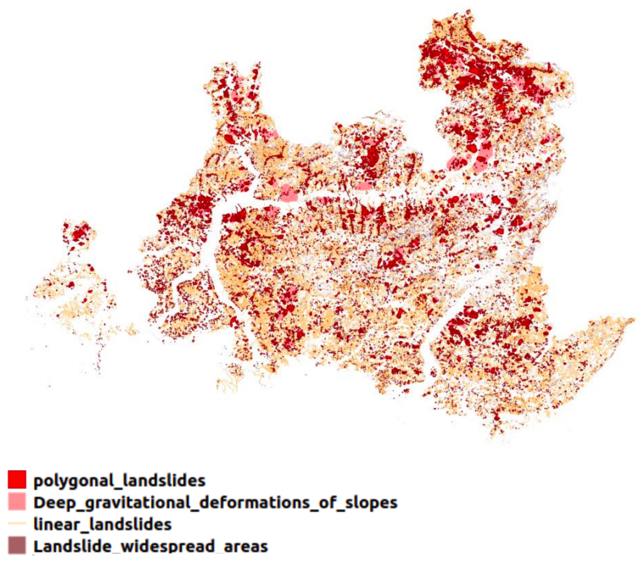
Figure 1.
Landslide distribution in Lombardy (Italy) according to the Geoportal of Lombardy.
Figure 1.
Landslide distribution in Lombardy (Italy) according to the Geoportal of Lombardy.
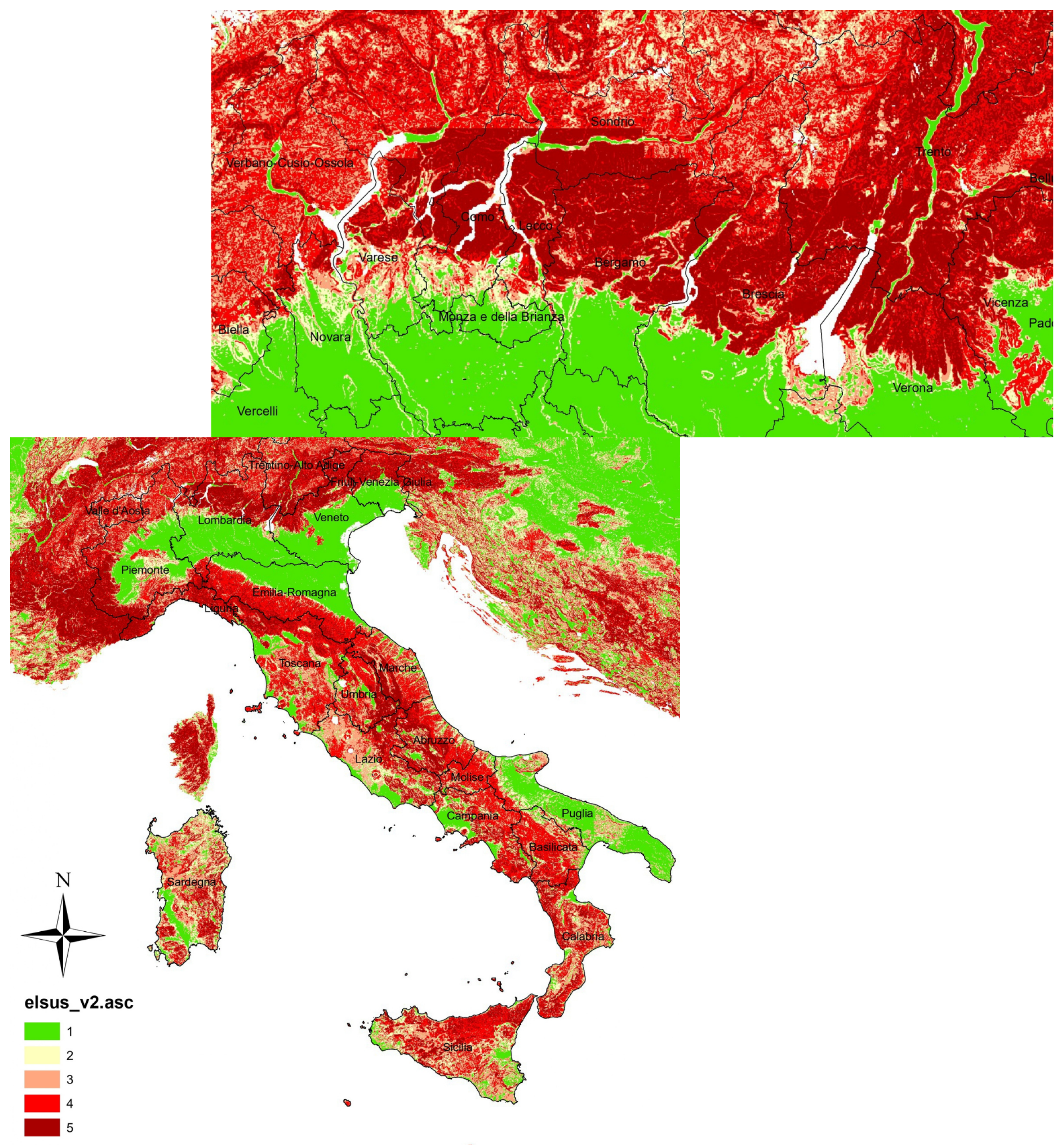
Figure 2.
European landslide susceptibility map (Italy, Lombardy) according to the European Soil Data Center. The colors from green to red represent the sensitivity degrees from low to high.
Figure 2.
European landslide susceptibility map (Italy, Lombardy) according to the European Soil Data Center. The colors from green to red represent the sensitivity degrees from low to high.
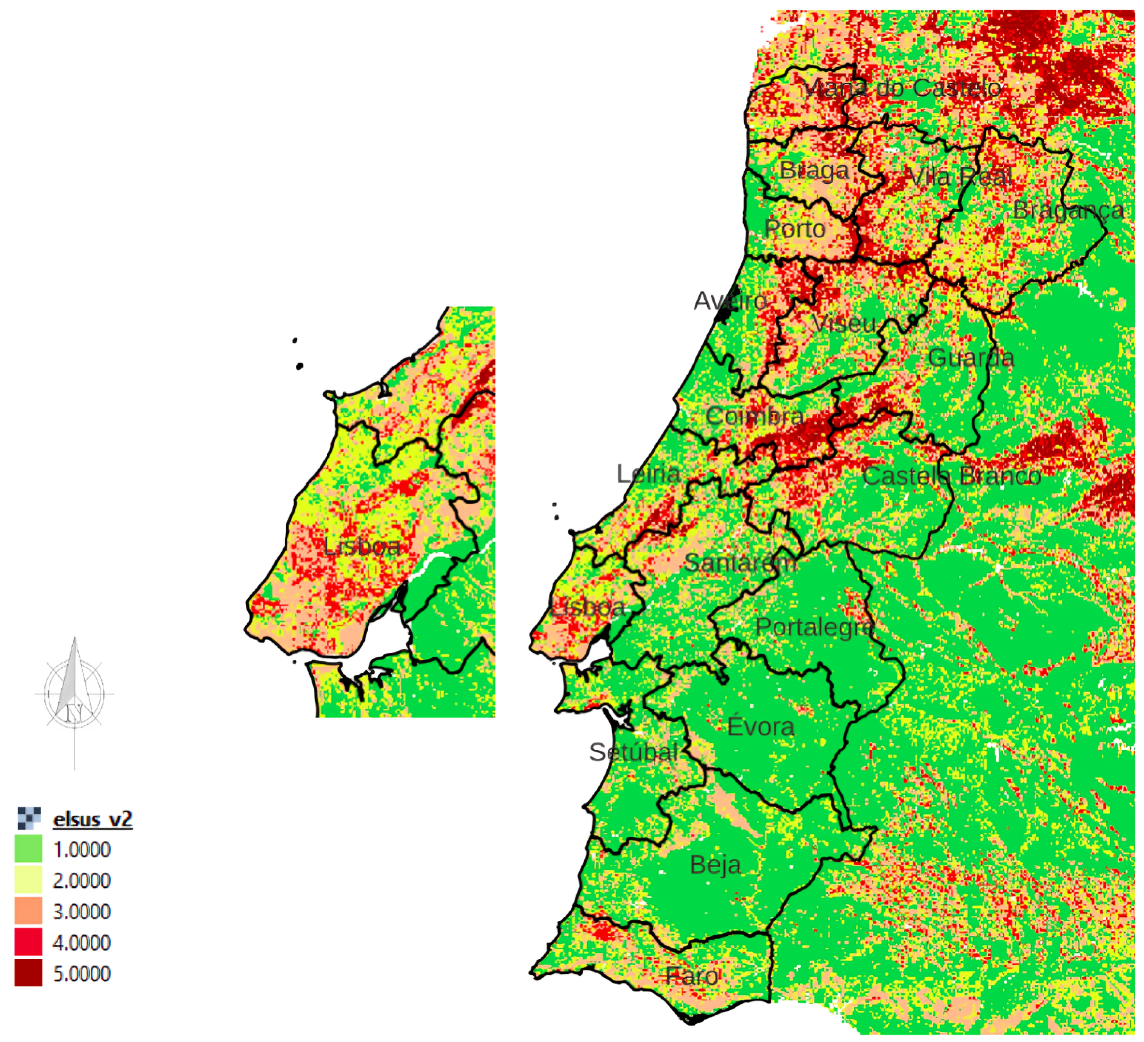
Figure 3.
European landslide susceptibility map (Portugal, Lisbon) according to the European Soil Data Center. The colors from green to red represent the sensitivity degrees from low to high.
Figure 3.
European landslide susceptibility map (Portugal, Lisbon) according to the European Soil Data Center. The colors from green to red represent the sensitivity degrees from low to high.
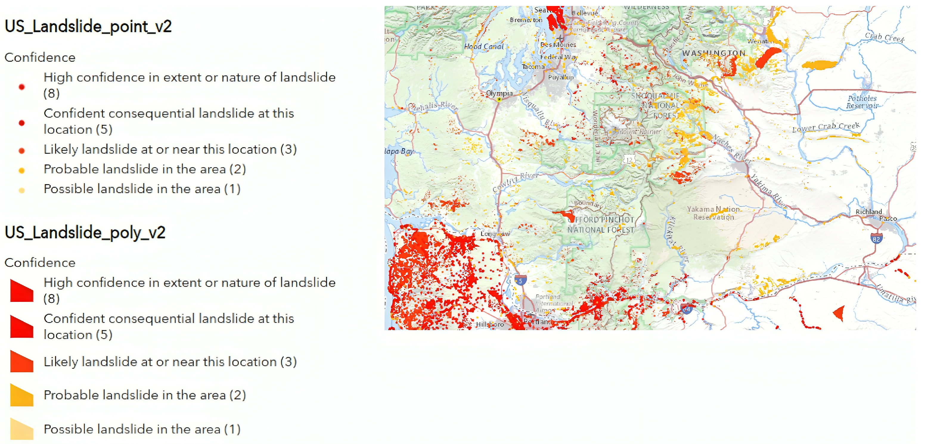
Figure 4.
Washington landslide susceptibility map according to the United States geological survey.
Figure 4.
Washington landslide susceptibility map according to the United States geological survey.
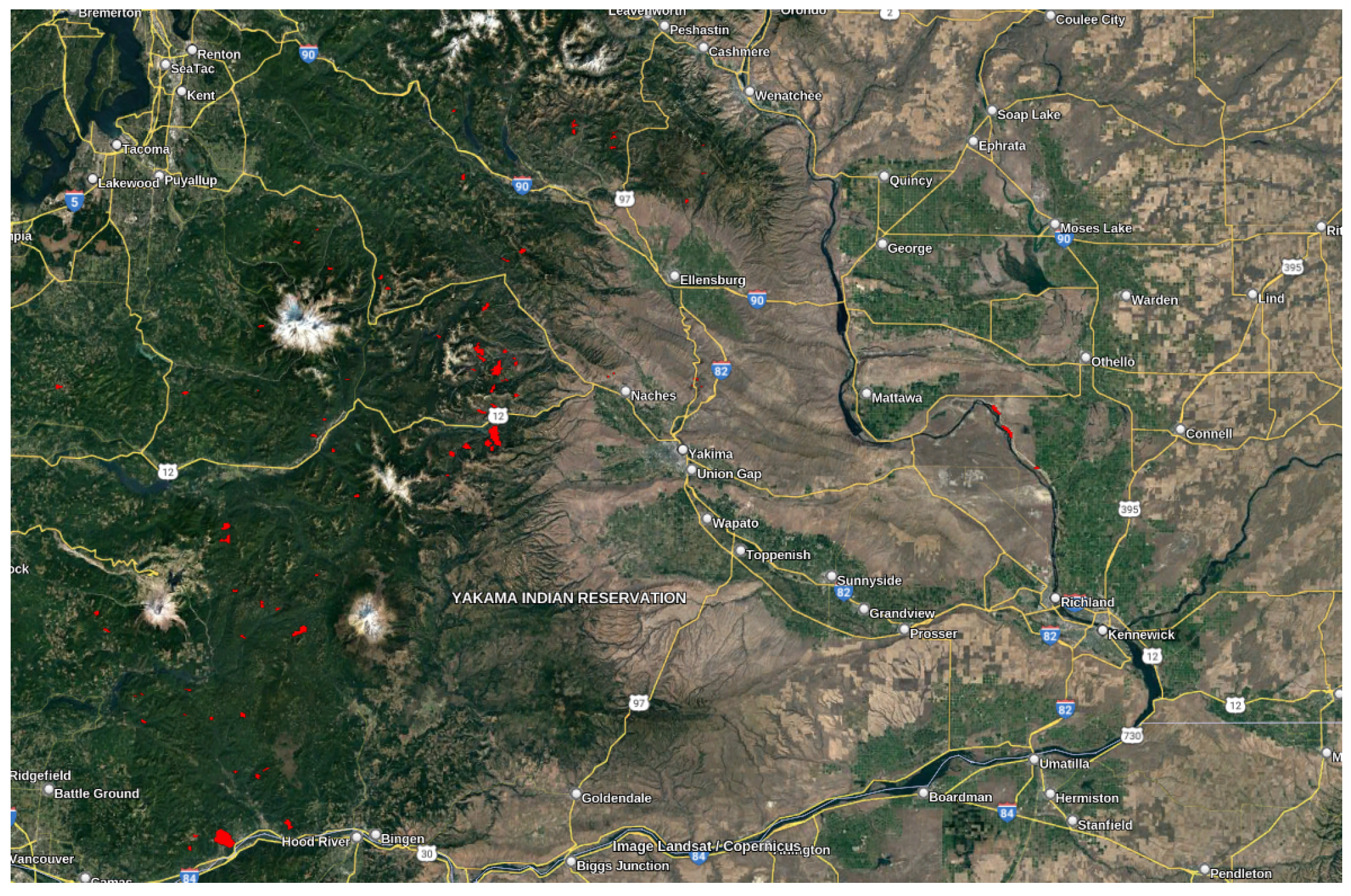
Figure 5.
Washington deep-seated landslides captured by ALOS-2 PALSAR-2 images between 2015 and 2019. The red polygons represent the landslide locations.
Figure 5.
Washington deep-seated landslides captured by ALOS-2 PALSAR-2 images between 2015 and 2019. The red polygons represent the landslide locations.
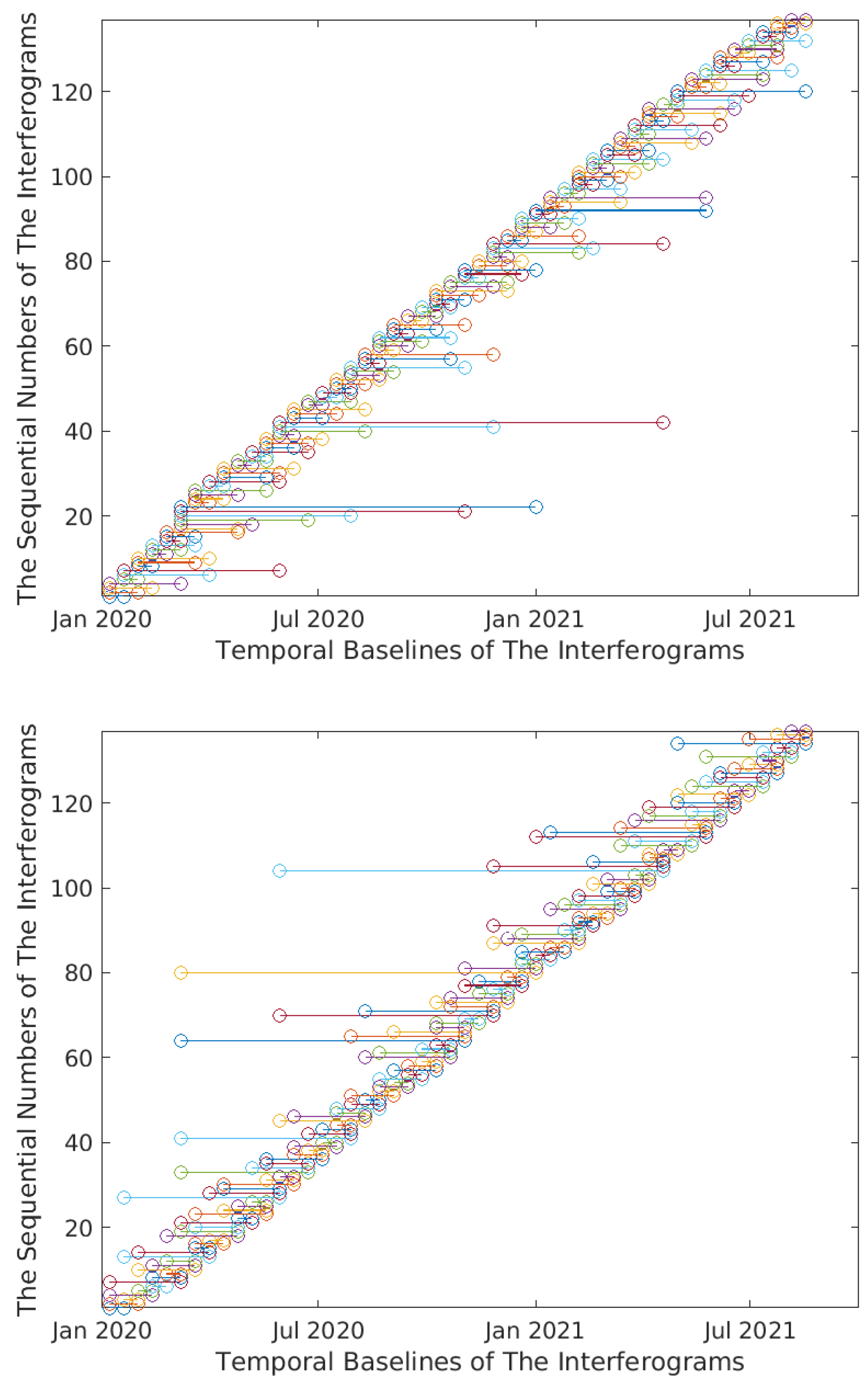
Figure 6.
The chronological sorting of the temporal baselines of the wrapped interferograms (Lombardy Dataset). Top figure expresses the sequence of the temporal baselines of the interferograms before sorting. Bottom figure expresses the sequence of the temporal baselines of the interferograms after sorting. Similar results have been obtained for the other two datasets of Lisbon and Washington.
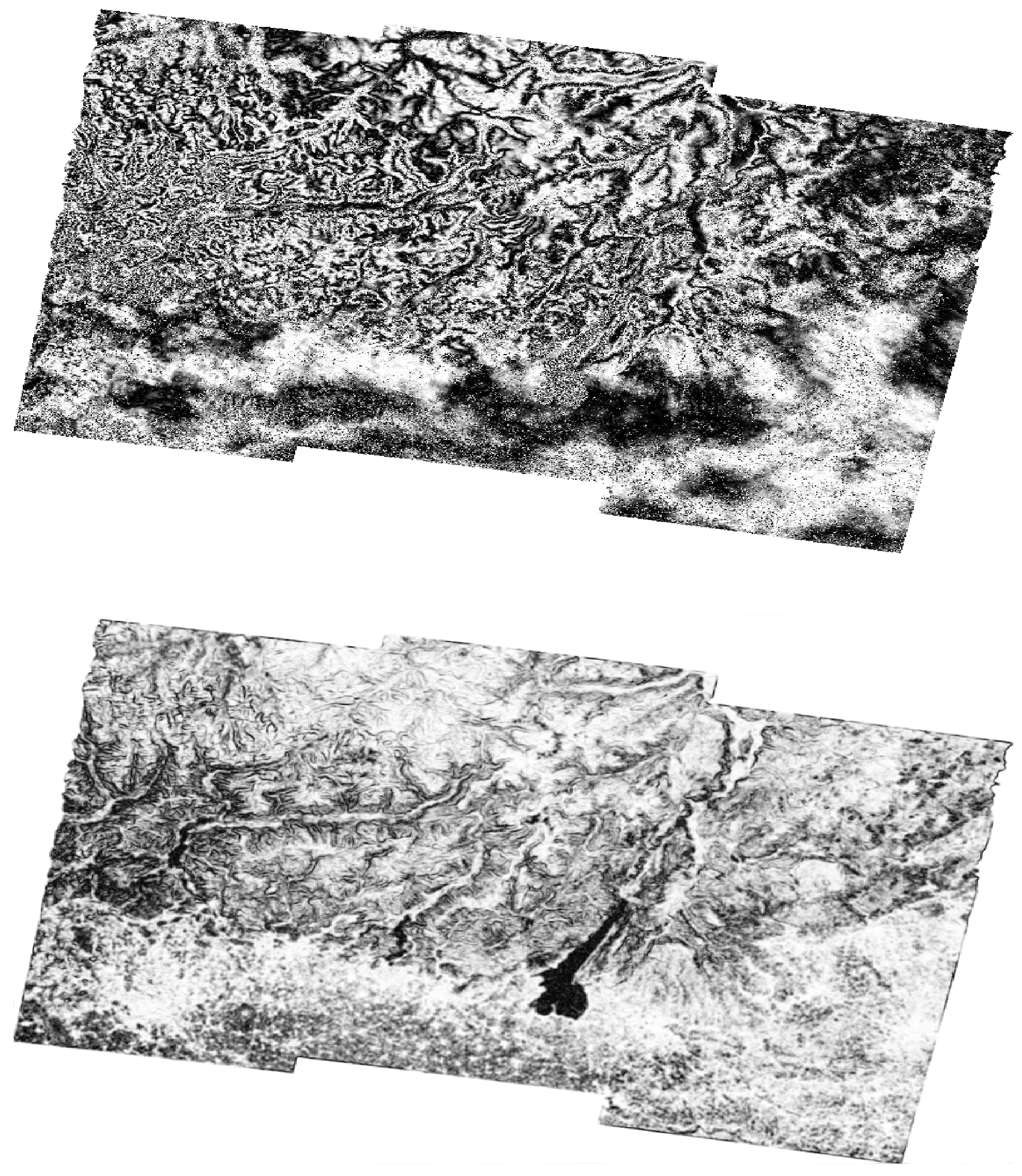
Figure 7.
Example of a wrapped interferogram in the complex domain from the Lombardy dataset before using the high-pass filter (top figure) and the magnitude after using the high-pass filter (bottom figure).
Figure 7.
Example of a wrapped interferogram in the complex domain from the Lombardy dataset before using the high-pass filter (top figure) and the magnitude after using the high-pass filter (bottom figure).
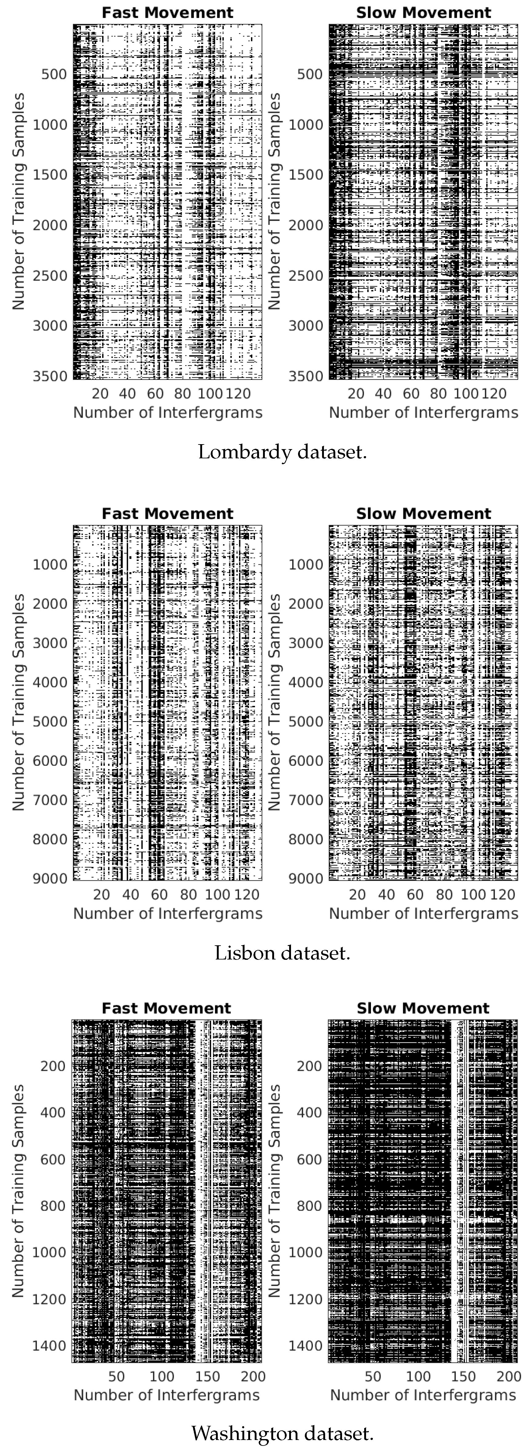
Figure 8.
The matrices represent slow and fast motions based on the used datasets. The black color in the matrices represents the magnitude values greater than 0.9 radians, while the white color represents the filtered phase values smaller than 0.9 radians.
Figure 8.
The matrices represent slow and fast motions based on the used datasets. The black color in the matrices represents the magnitude values greater than 0.9 radians, while the white color represents the filtered phase values smaller than 0.9 radians.
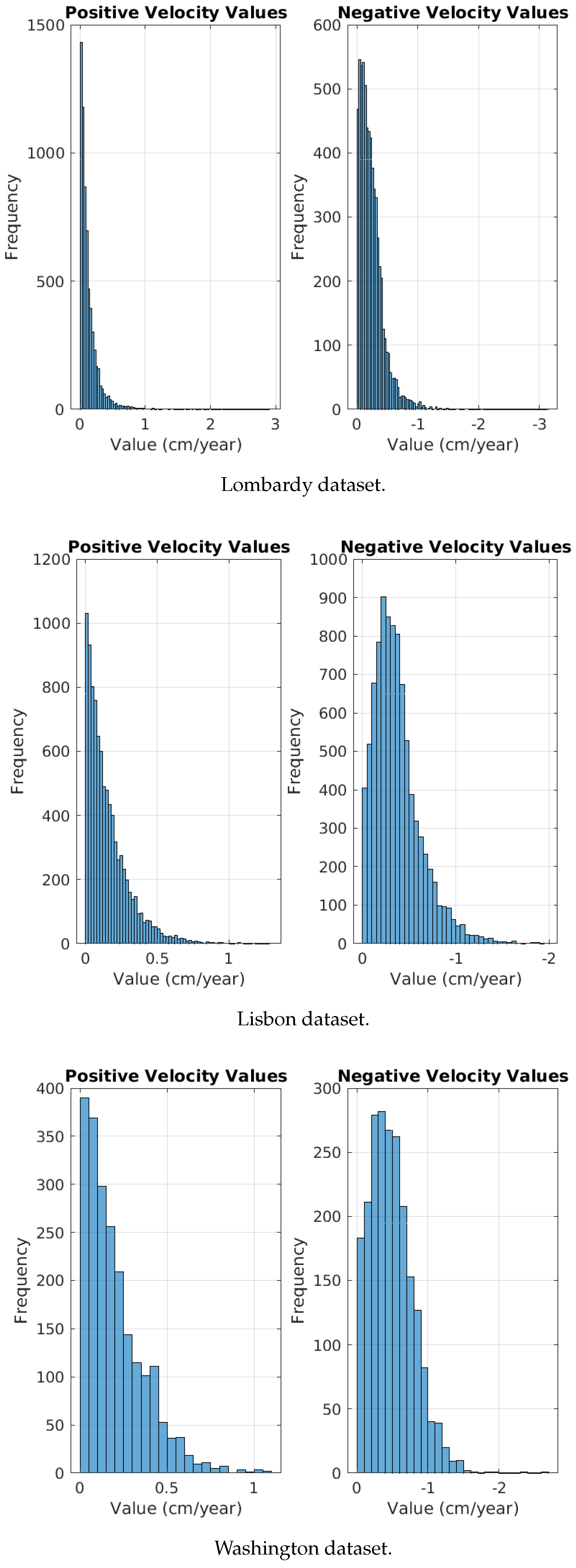
Figure 9.
The histograms representing positive and negative motions based on the used datasets.
Figure 9.
The histograms representing positive and negative motions based on the used datasets.
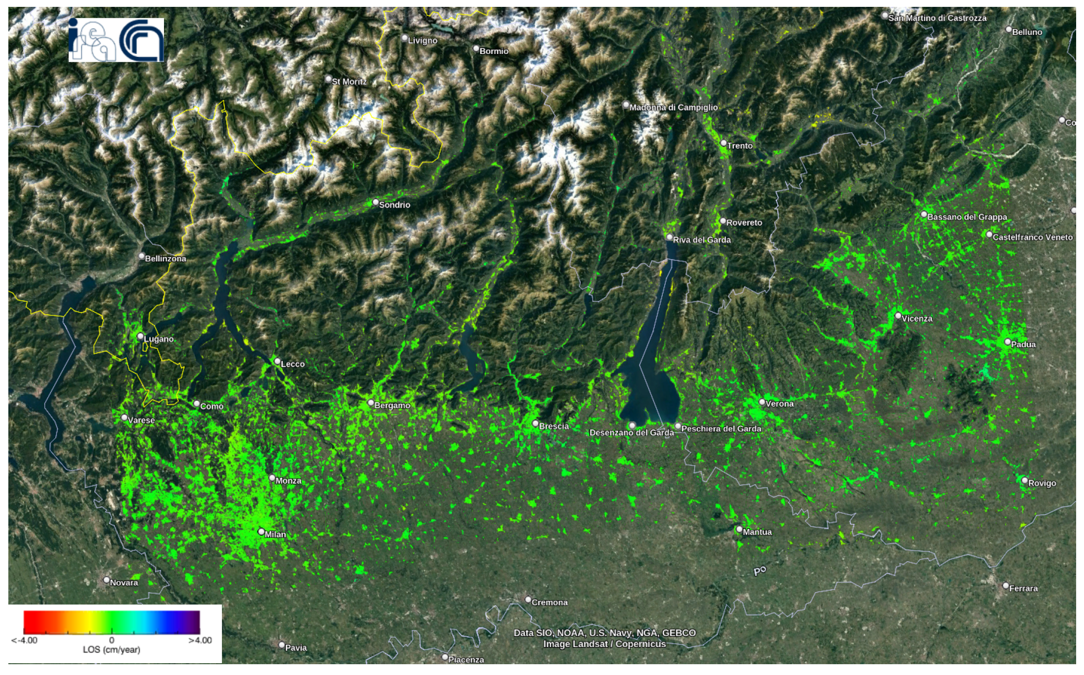
Figure 10.
Deformation orm as it is so keep velocity map of the Lombardy dataset using the P-SBAS service at the G-TEP.
Figure 10.
Deformation orm as it is so keep velocity map of the Lombardy dataset using the P-SBAS service at the G-TEP.
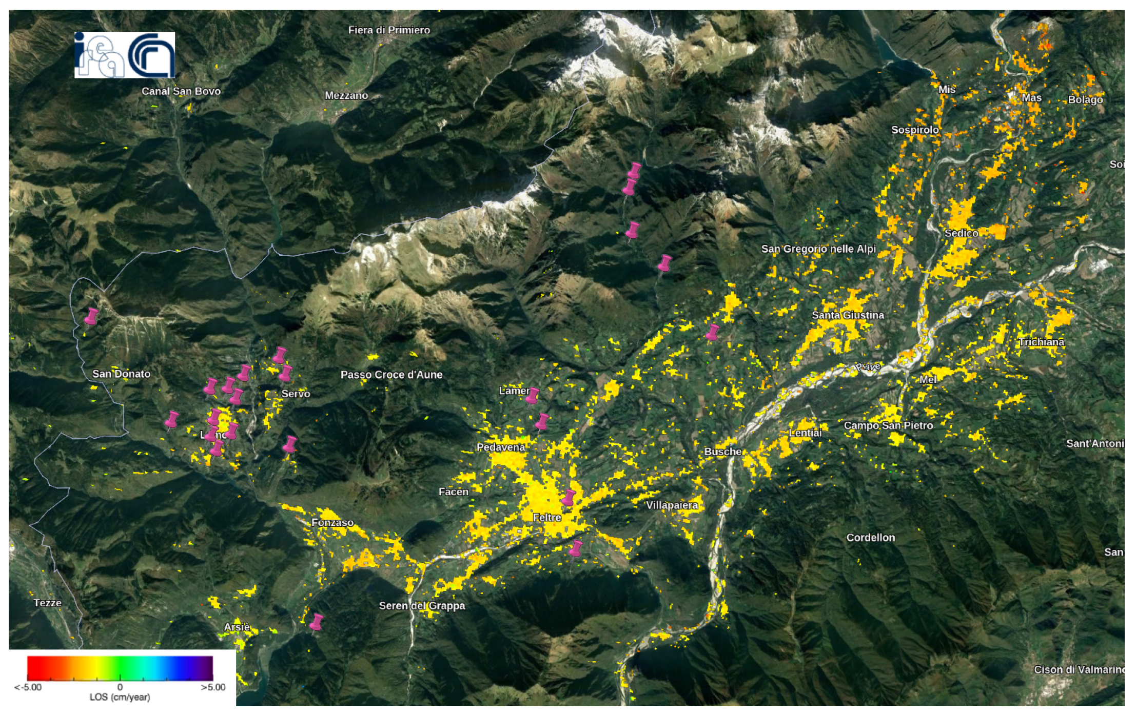
Figure 11.
Intersection between S.Puliero et al.’s landslide dataset and the Sentinel-1 deformation velocity map in Belluno [
41]. The violet pins refer to the location of the landslides.
Figure 11.
Intersection between S.Puliero et al.’s landslide dataset and the Sentinel-1 deformation velocity map in Belluno [
41]. The violet pins refer to the location of the landslides.
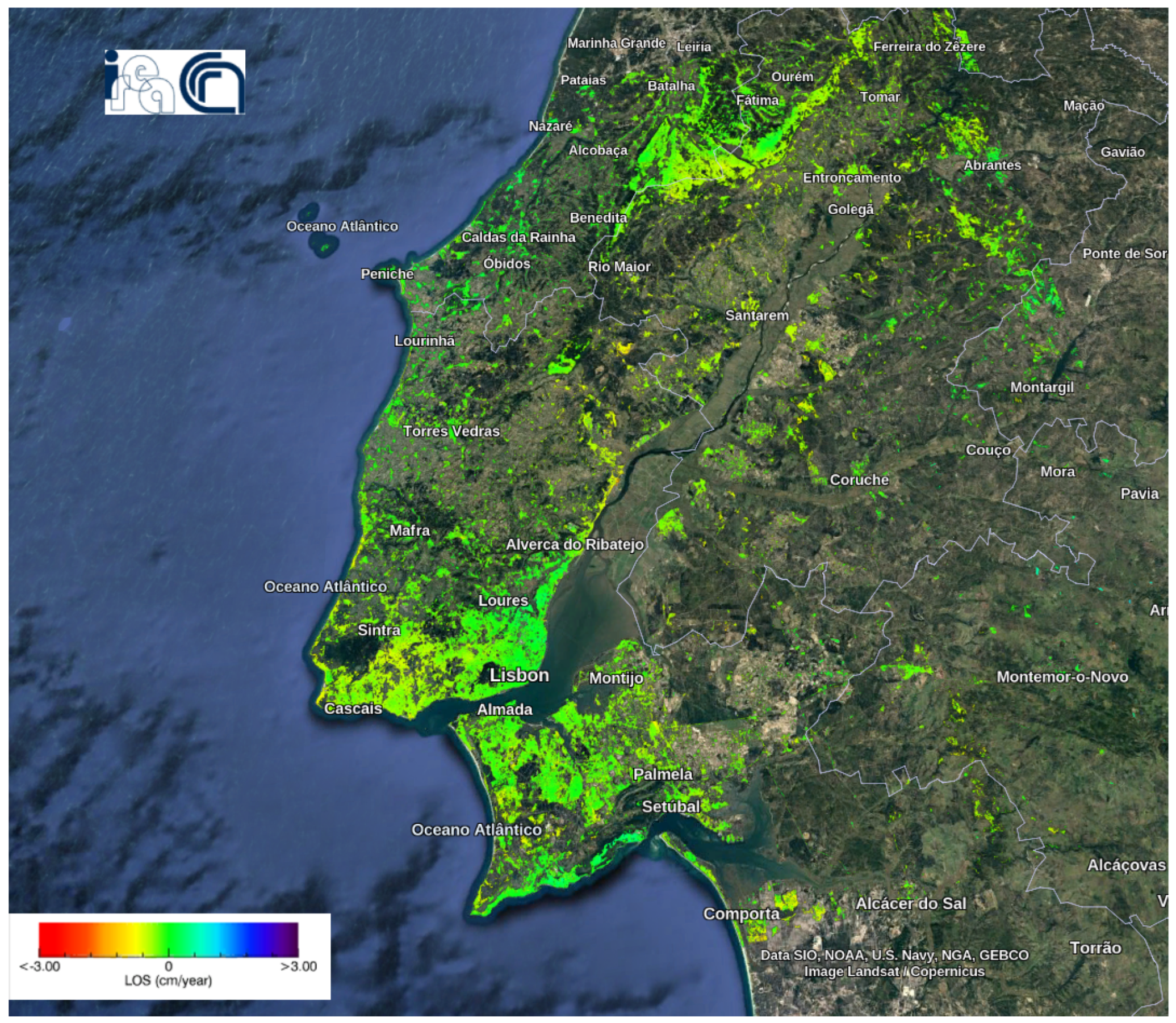
Figure 12.
Deformation velocity map of the Lisbon dataset using the P-SBAS service at the G-TEP.
Figure 12.
Deformation velocity map of the Lisbon dataset using the P-SBAS service at the G-TEP.
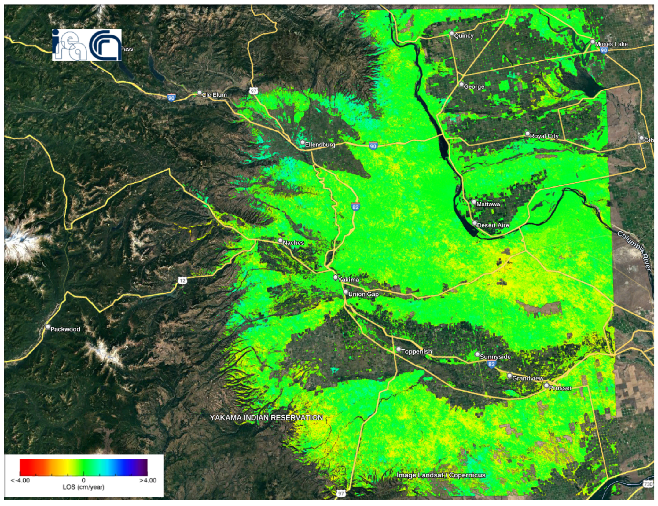
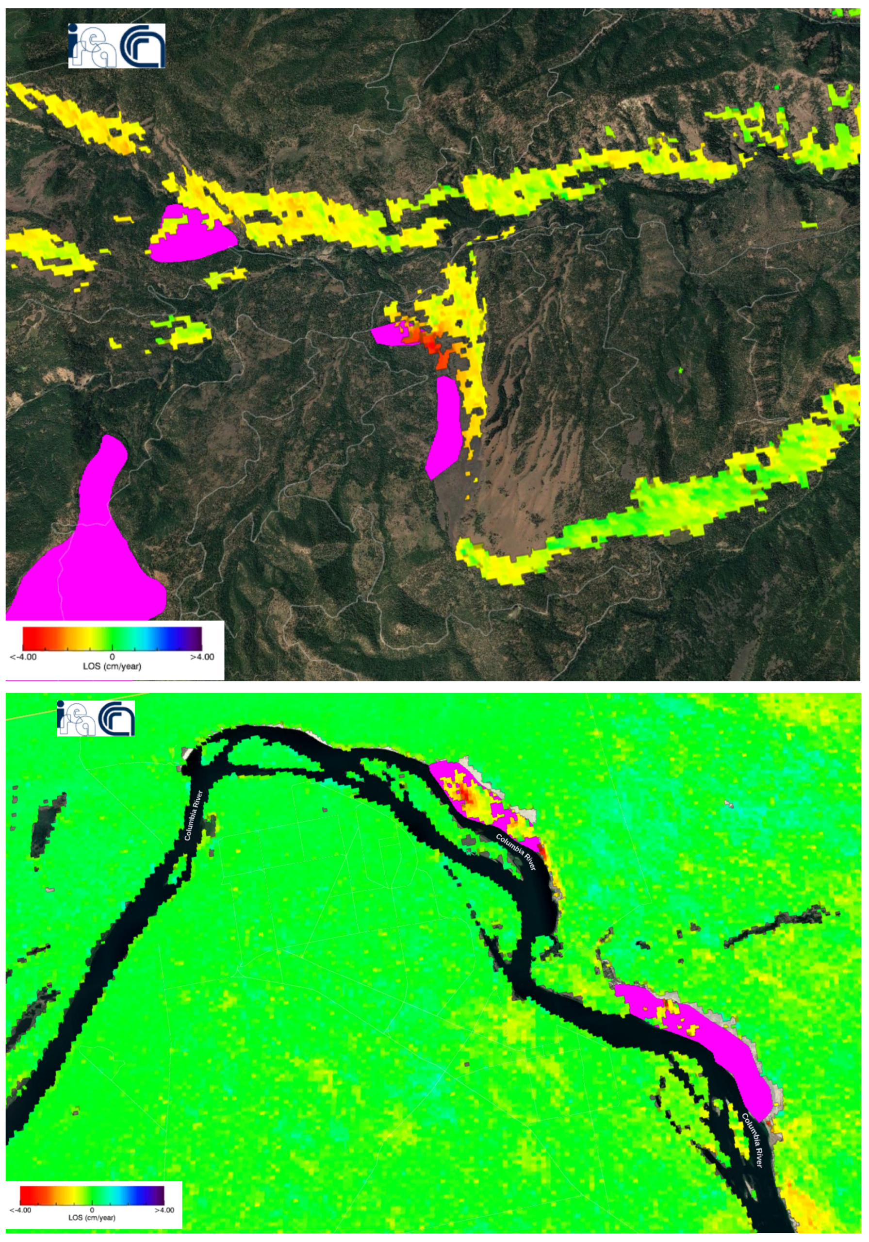
Figure 13.
Deformation velocity map of the Washington dataset using the P-SBAS service at the G-TEP.
Figure 13.
Deformation velocity map of the Washington dataset using the P-SBAS service at the G-TEP.
Figure 14.
Intersections between landslides dataset [
24] and deformation velocity map in the Washington U.S. The violet polygons represent the landslides dataset.
Figure 14.
Intersections between landslides dataset [
24] and deformation velocity map in the Washington U.S. The violet polygons represent the landslides dataset.
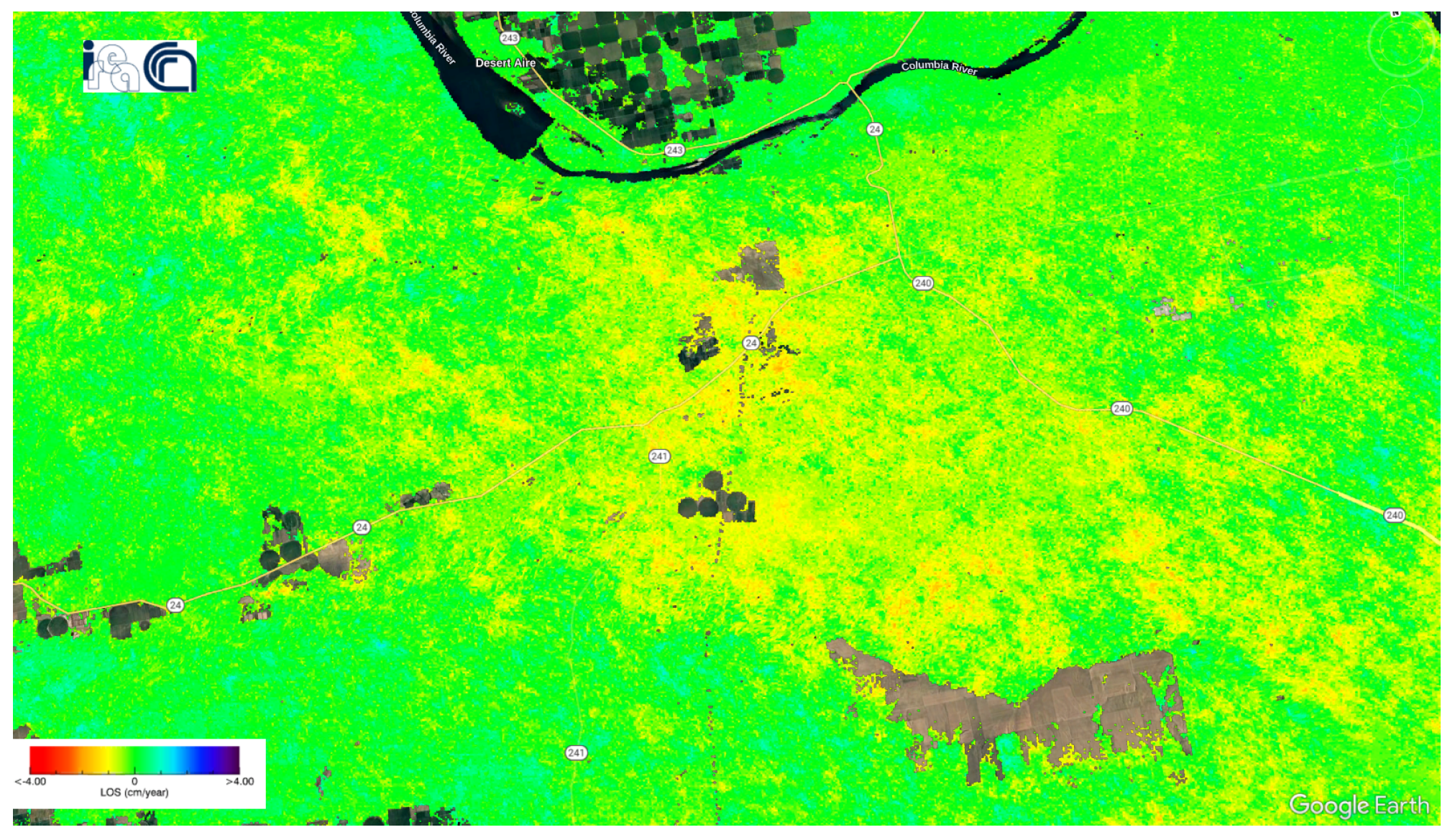
Figure 15.
Deformation velocity map of zone 98,944 according to the time series analysis of the Washington dataset.
Figure 15.
Deformation velocity map of zone 98,944 according to the time series analysis of the Washington dataset.
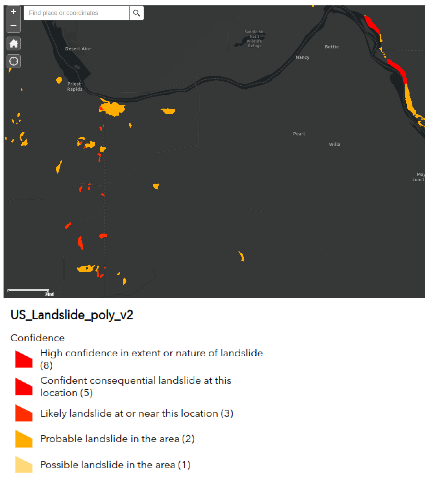
Figure 16.
Sensitivity map to landslides in zone 98,944 according to the U.S. Landslide Inventory Web Application.
Figure 16.
Sensitivity map to landslides in zone 98,944 according to the U.S. Landslide Inventory Web Application.
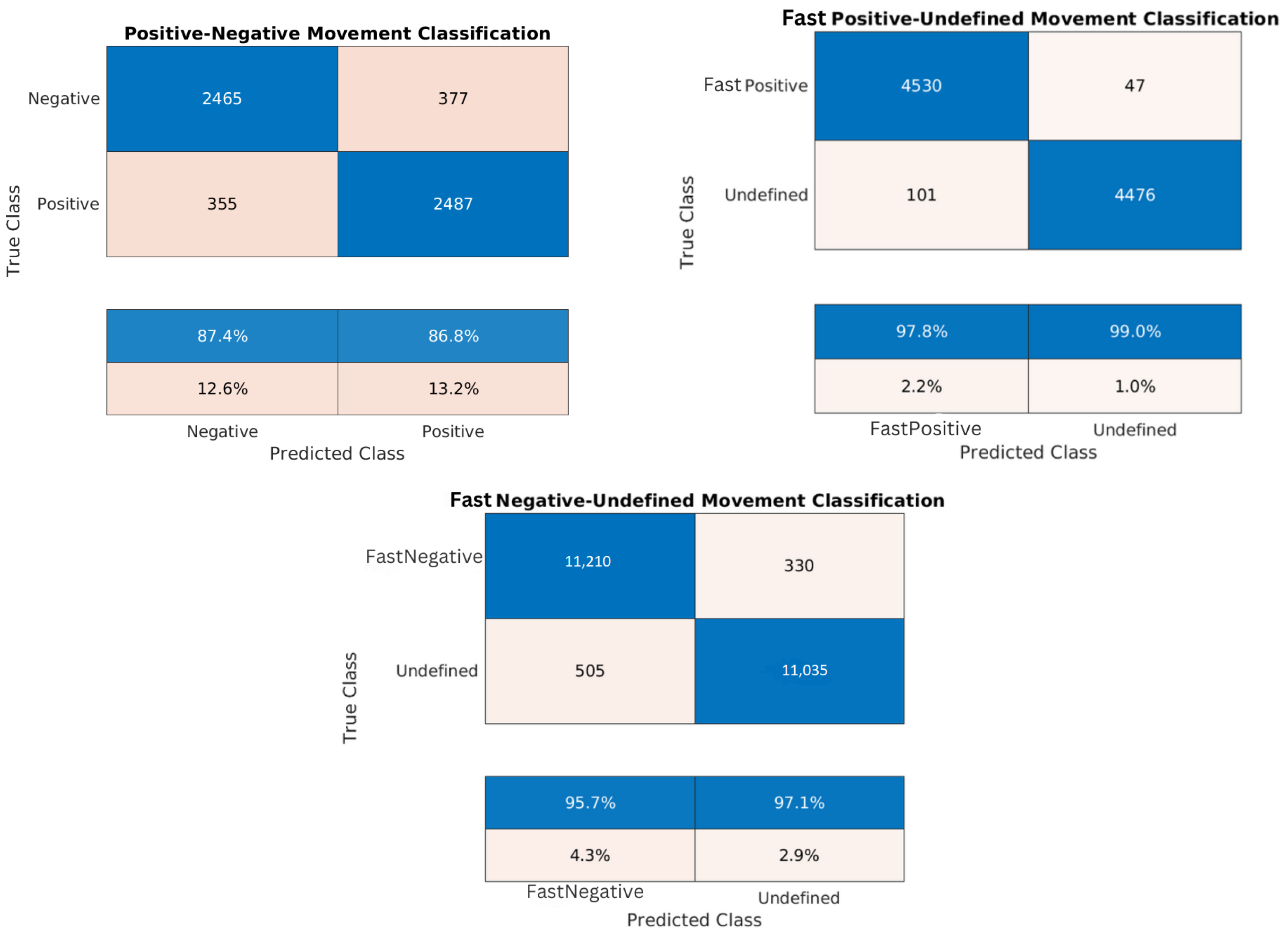
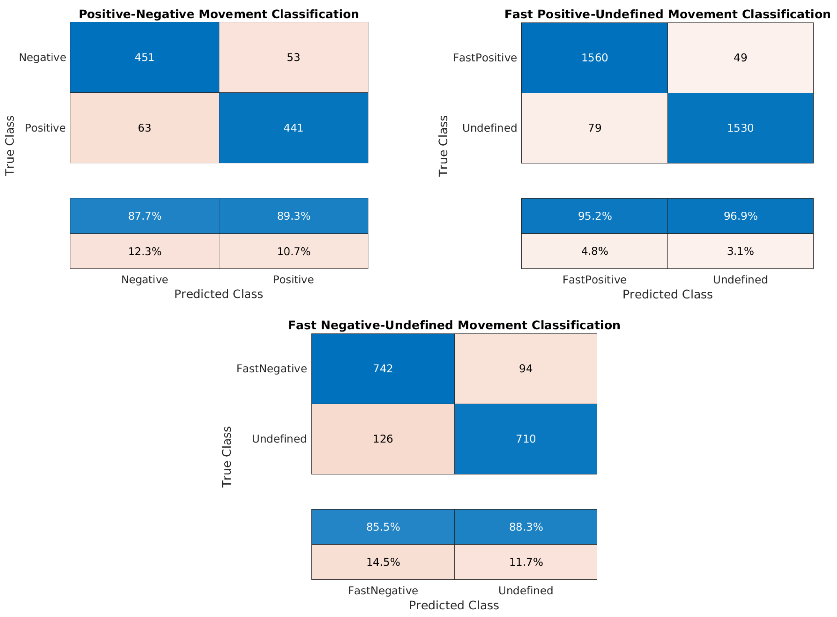
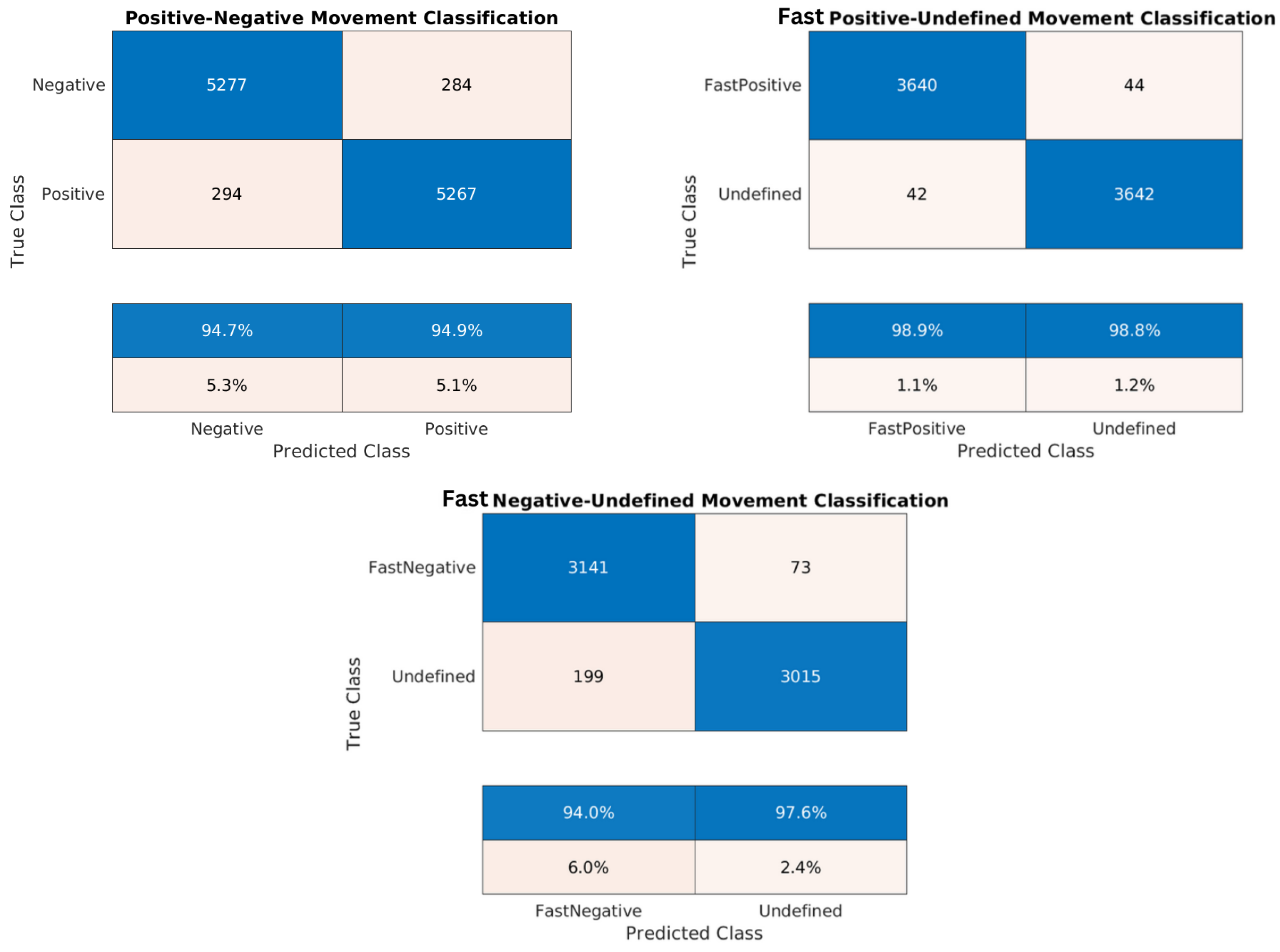
Figure 17.
Confusion matrices for the trained models of the Lombardy dataset: positive/negative movement model, fast positive movement model, and fast negative movement model, respectively.
Figure 17.
Confusion matrices for the trained models of the Lombardy dataset: positive/negative movement model, fast positive movement model, and fast negative movement model, respectively.
Figure 18.
Confusion matrices for the trained models of the Lisbon dataset: positive/negative movement model, fast positive movement model, and fast negative movement model, respectively.
Figure 18.
Confusion matrices for the trained models of the Lisbon dataset: positive/negative movement model, fast positive movement model, and fast negative movement model, respectively.
Figure 19.
Confusion matrices for the trained models of the Washington dataset: positive/negative movement model, fast positive movement model, and fast negative movement model, respectively.
Figure 19.
Confusion matrices for the trained models of the Washington dataset: positive/negative movement model, fast positive movement model, and fast negative movement model, respectively.
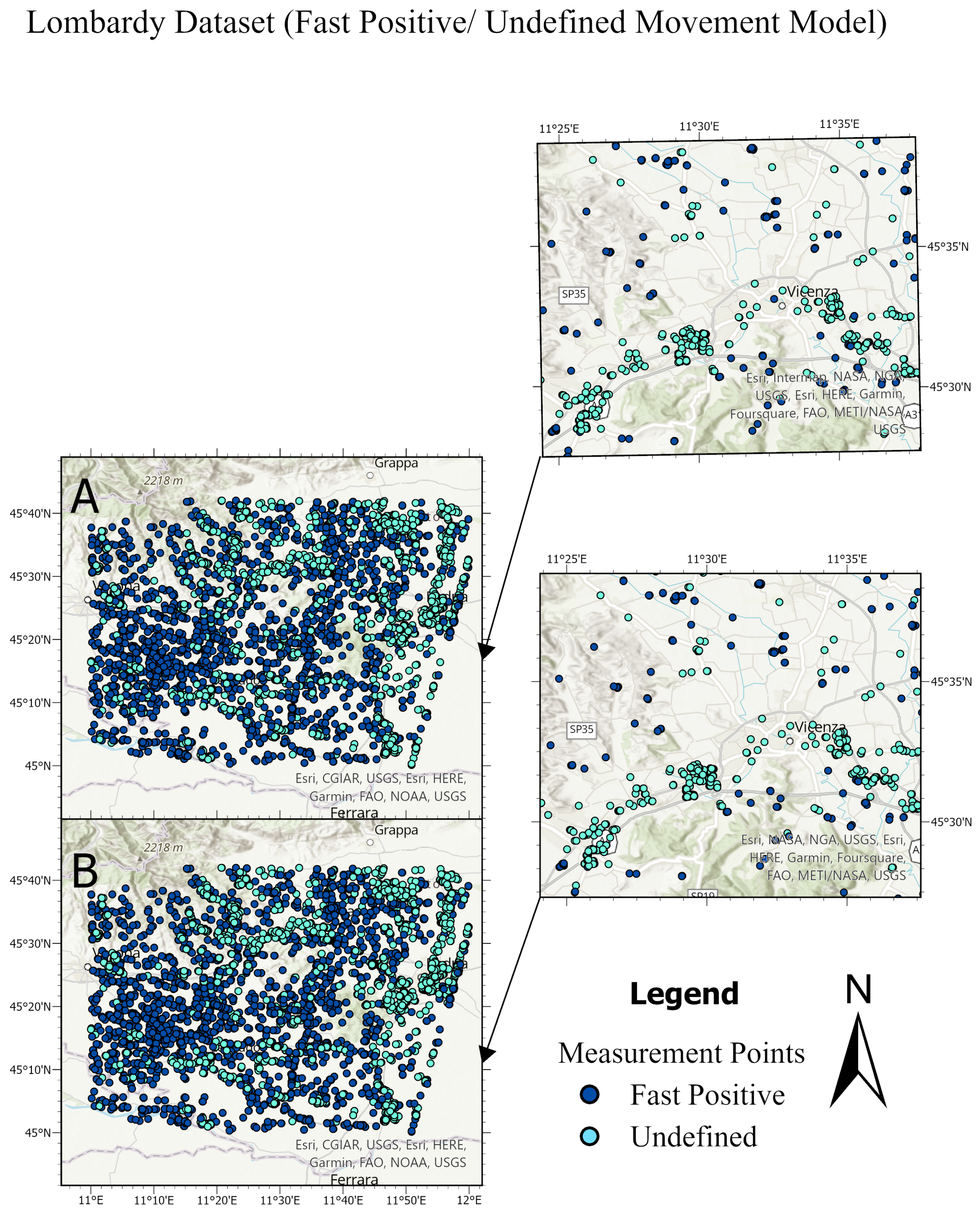
Figure 20.
Comparison between the ground truth and the predictions of the test sets for different datasets. Top main figure: Lombardy dataset, showing fast positive and undefined movements. Bottom main figure: Lisbon dataset, displaying positive and negative movements. Each main figure consists of four subfigures. In the top subfigure, Subfigure (A) presents the ground truth of the Lombardy test set, with Subfigure (a) providing a detailed close-up of Subfigure (A). Subfigure (B) shows the predictions for the Lombardy test set, with Subfigure (b) offering a close-up of these predictions. Similarly, in the bottom main figure for the Lisbon dataset, Subfigure (A) and Subfigure (a) focus on the ground truth test set and its close-up, respectively, while Subfigure (B) and Subfigure (b) depict the predictions and their close-up.
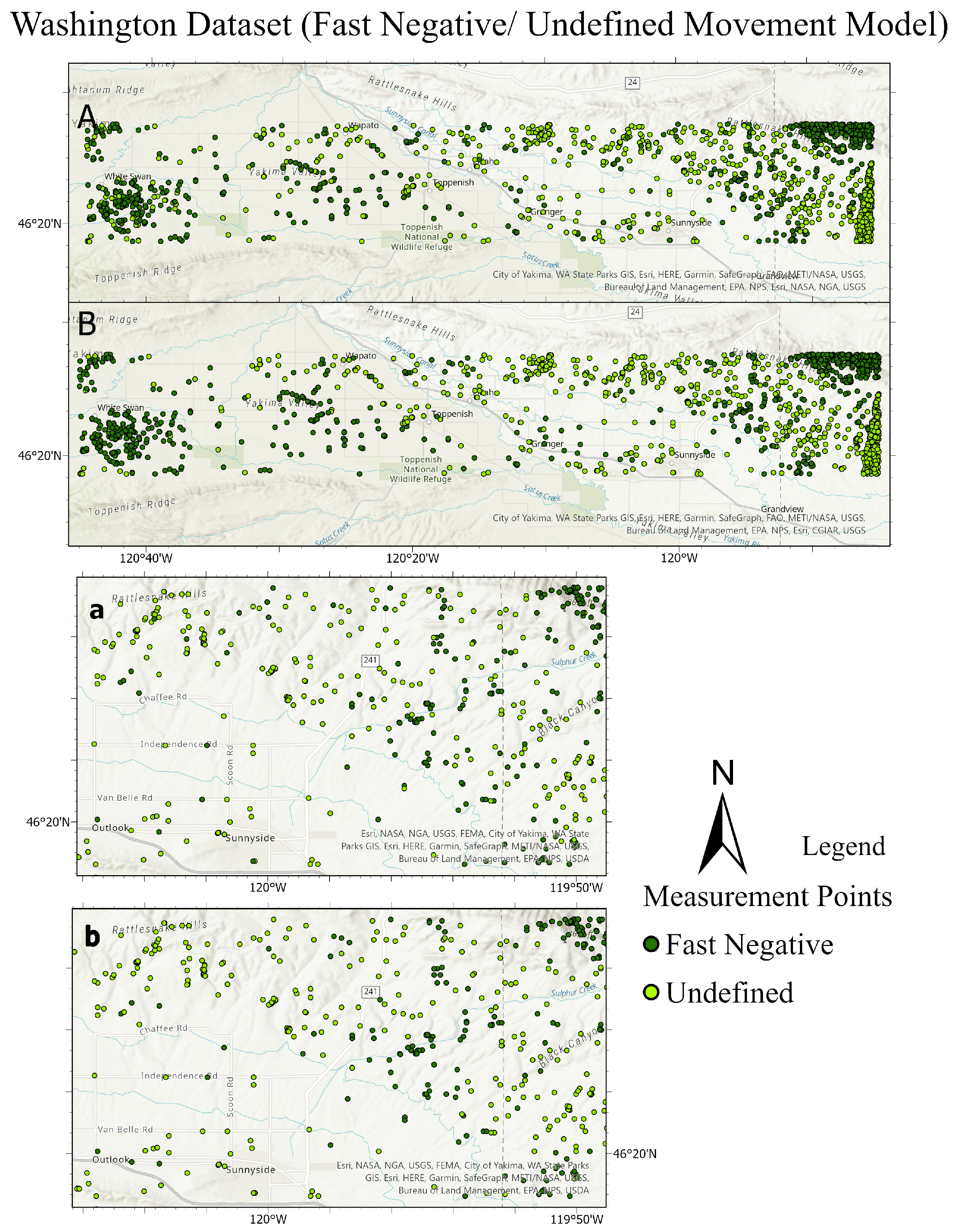
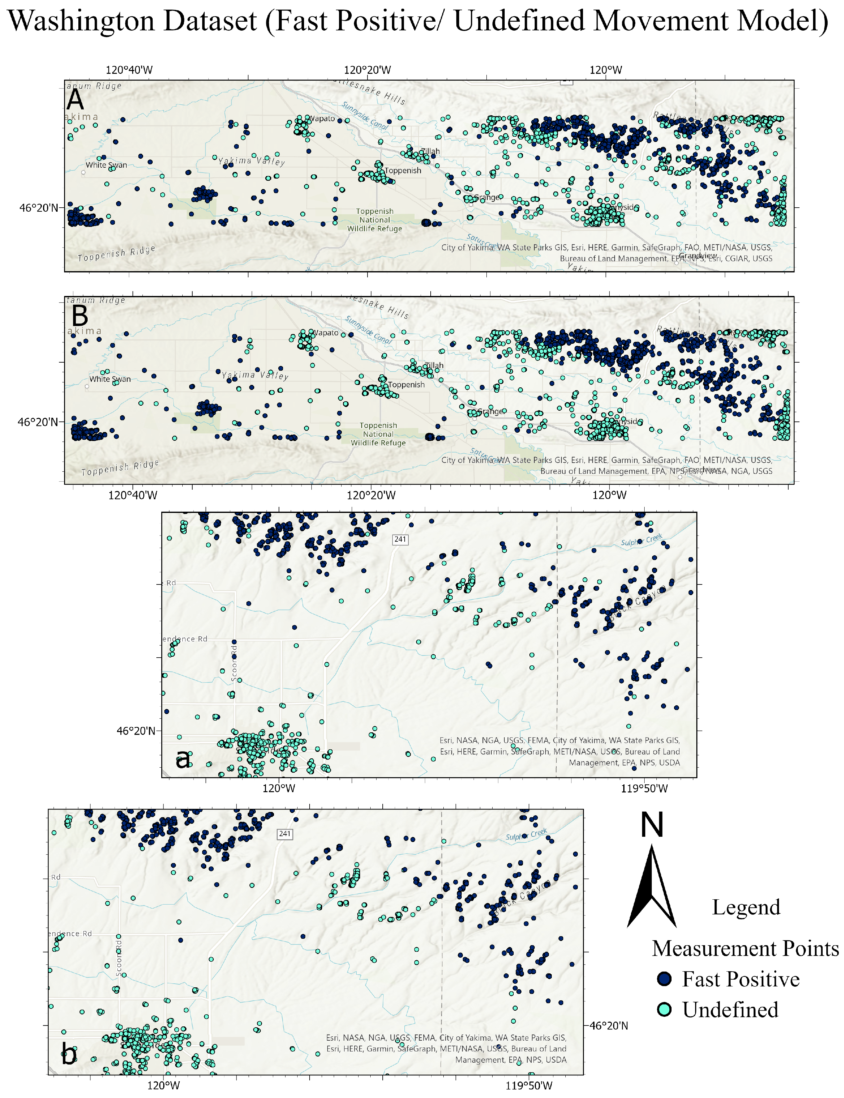
Figure 21.
Comparison of the ground truth test set and its predictions for the Washington dataset. The top figure illustrates fast negative and undefined movements, while the bottom figure shows fast positive and undefined movements. In each figure, subfigure A depicts the ground truth of the test dataset, and subfigure a provides a detailed close-up of A. Subfigure B presents the predictions for the test dataset, with subfigure b offering a close-up view of B.
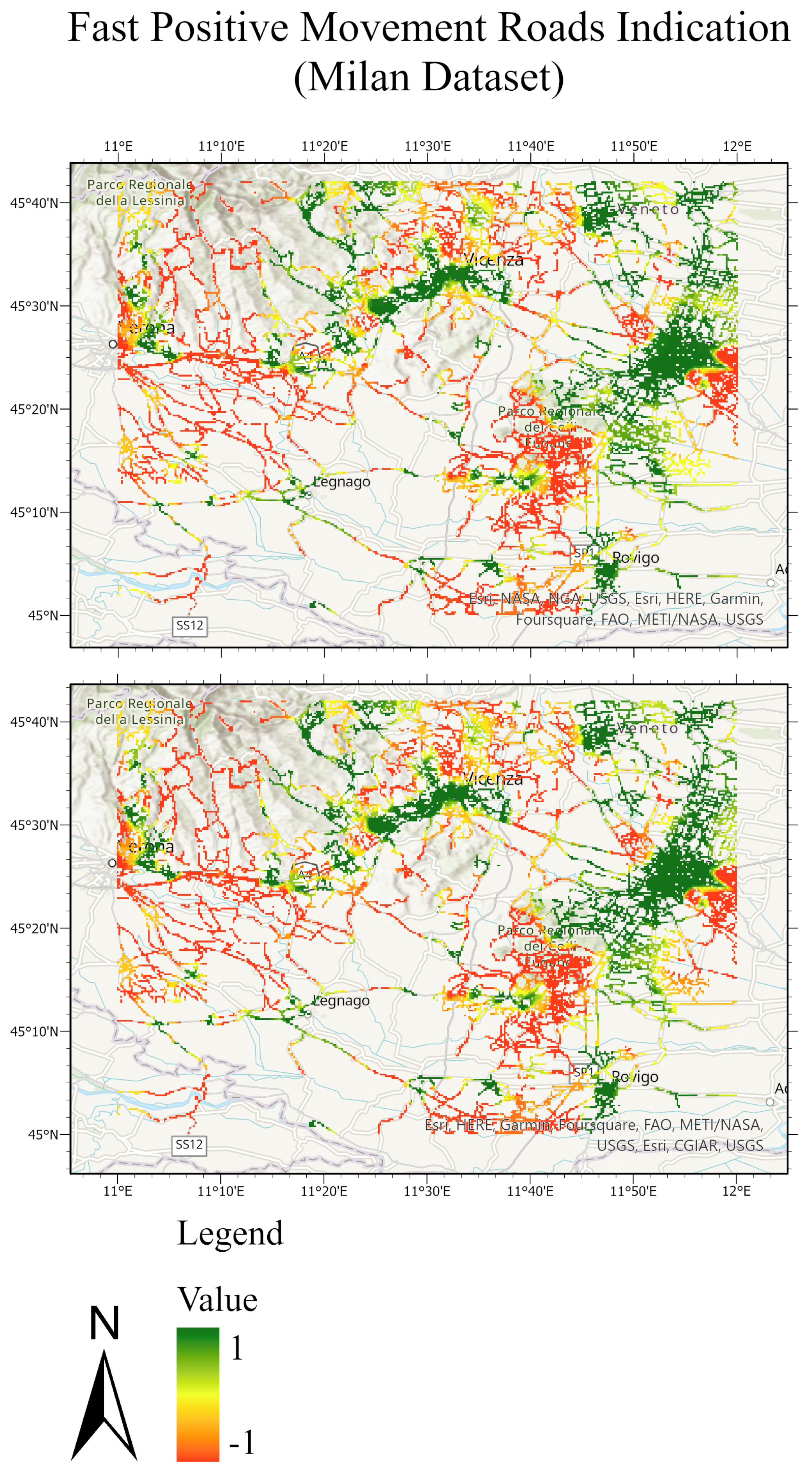
Figure 22.
Road network of the Lombardy test dataset. The top figure exhibits the masked roads of the ground truth test set; the bottom figure exhibits the masked roads of the predicted test sets. The value of −1 expresses the fast positive movement while the value of 1 expresses the undefined movement.
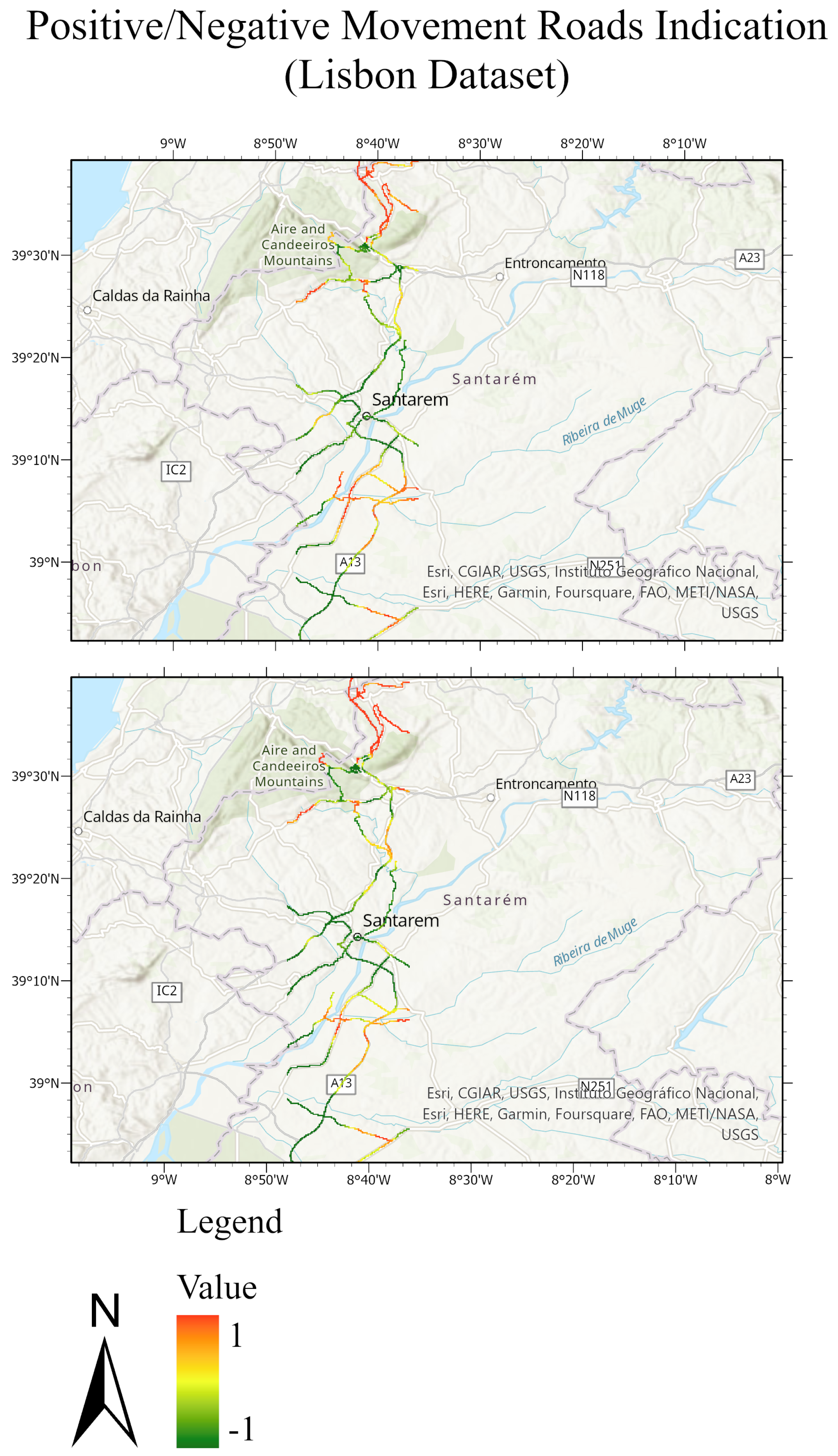
Figure 23.
Road network of the Lisbon test dataset. The masked roads of the ground truth test set are shown in the top figure; while the masked roads of the predicted test sets are shown in the bottom figure. The value of 1 expresses the positive movement while the value −1 expresses the negative movement.
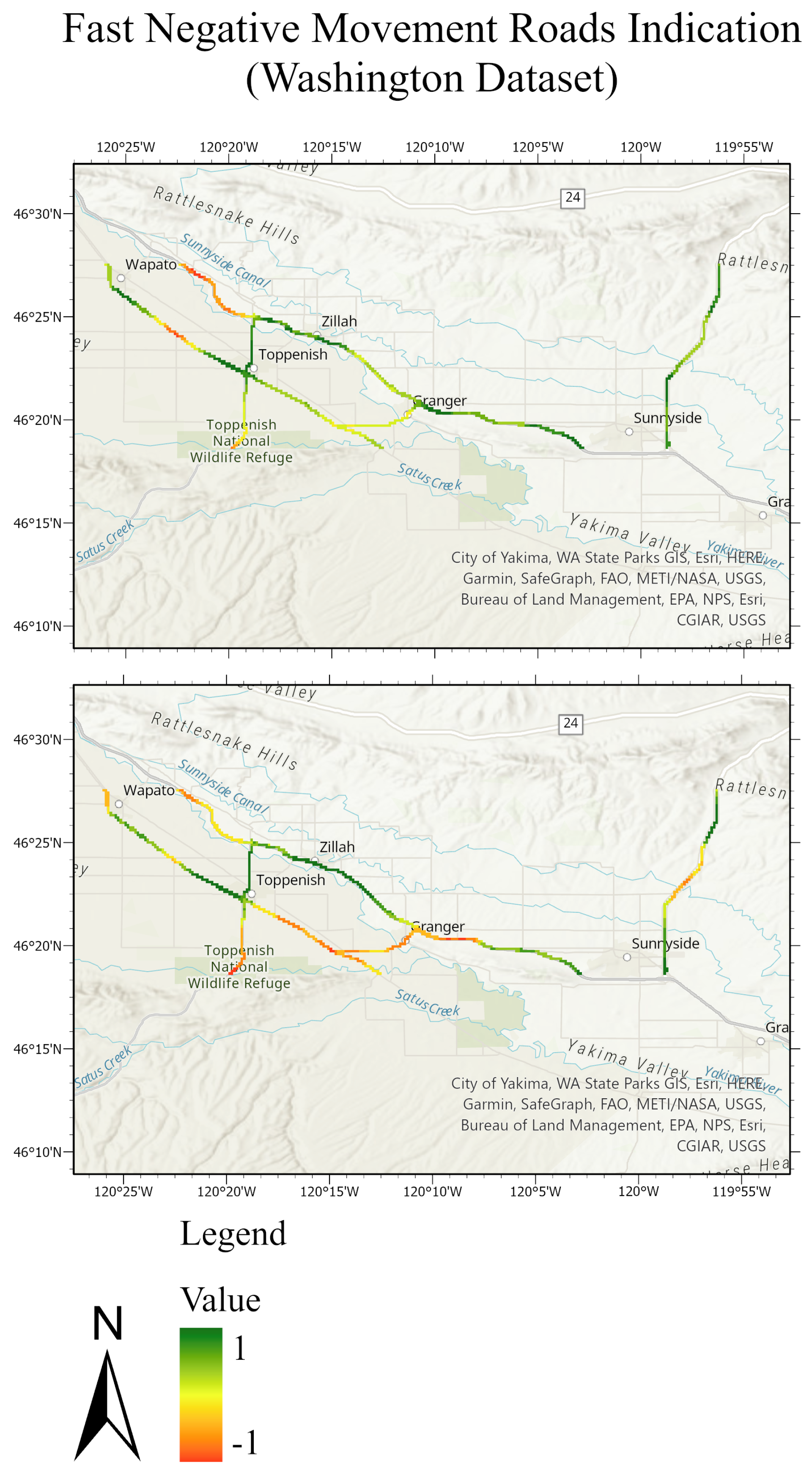
Figure 24.
Road network of the Washington test dataset. The top figure represents the masked roads of the ground truth test set; the bottom figure represents the masked roads of the predicted test sets. The value of −1 expresses the fast negative movement while the value of 1 expresses the undefined movement.
Table 1.
The selected parameters of the P-SBAS analysis for Lombardy (Italy) dataset.
Table 1.
The selected parameters of the P-SBAS analysis for Lombardy (Italy) dataset.
| Start Date | 7 January 2020 |
| End Date | 17 August 2021 |
| Number of Images | 50 |
| DEM | SRTM1 arcsec |
| Temporal Coherence | 0.85 |
| Bounding Box | 44.943, 8.693 |
| | 46.884, 12.231 |
| Orbit Direction | Descending |
Table 2.
The selected parameters of the P-SBAS analysis for the Lisbon (Portugal) dataset.
Table 2.
The selected parameters of the P-SBAS analysis for the Lisbon (Portugal) dataset.
| Start Date | 26 January 2018 |
| End Date | 27 April 2020 |
| Number of Images | 50 |
| DEM | SRTM1 arcsec |
| Temporal Coherence | 0.6 |
| Bounding Box | 38.088, −11.124 |
| | 39.800, −7.945 |
| Orbit Direction | Ascending |
Table 3.
The selected parameters of the P-SBAS analysis for the Washington dataset.
Table 3.
The selected parameters of the P-SBAS analysis for the Washington dataset.
| Start Date | 14 October 2016 |
| End Date | 28 December 2019 |
| Number of Images | 75 |
| DEM | SRTM1 arcsec |
| Temporal Coherence | 0.7 |
| Bounding Box | −121.426, 46.358 |
| | −120.042, 47.167 |
| Orbit Direction | Ascending |
Table 4.
The statistical enumeration of data points obtained from the fast negative/undefined Milan dataset.
Table 4.
The statistical enumeration of data points obtained from the fast negative/undefined Milan dataset.
| Milan Dataset |
|---|
| Rate of Movement | From 0 To 0.9 Rad | From 0.9 To 1 Rad |
|---|
| FAST | 73.64% | 26.36% |
| SLOW | 58.80% | 41.20% |
Table 5.
The statistical enumeration of data points obtained from the fast negative/undefined Lisbon dataset.
Table 5.
The statistical enumeration of data points obtained from the fast negative/undefined Lisbon dataset.
| Lisbon Dataset |
|---|
| Rate of Movement | From 0 To 0.9 Rad | From 0.9 To 1 Rad |
|---|
| FAST | 72.81% | 27.19% |
| SLOW | 63.68% | 36.32% |
Table 6.
The statistical enumeration of data points obtained from the fast negative/undefined Washington dataset.
Table 6.
The statistical enumeration of data points obtained from the fast negative/undefined Washington dataset.
| Washington Dataset |
|---|
| Rate of Movement | From 0 To 0.9 Rad | From 0.9 To 1 Rad |
|---|
| FAST | 37.22% | 62.78% |
| SLOW | 26.29% | 73.71% |
Table 7.
Positive/negative movement model of the Lombardy dataset.
Table 7.
Positive/negative movement model of the Lombardy dataset.
| | Cosine K-NN | 1st PS | 2nd PS |
|---|
| Number of training samples | 10,382 | 36,596 | 44,488 |
| Number of testing samples | 2596 | 9148 | 11,122 |
| Accuracy of validation | 75% | 93.4% | 94.4% |
| Accuracy of the test set | 75.2% | 93.3% | 94.8% |
Table 8.
Fast negative/undefined movement model of the Lombardy dataset.
Table 8.
Fast negative/undefined movement model of the Lombardy dataset.
| | Cosine K-NN | 1st PS | 2nd PS | 3rd PS |
|---|
| Number of training samples | 7442 | 16,878 | 22,556 | 25,716 |
| Number of testing samples | 1860 | 4220 | 5640 | 6428 |
| Accuracy of validation | 85.3% | 93.3% | 95% | 95.6% |
| Accuracy of the test set | 84.4% | 93.5% | 95% | 95.8% |
Table 9.
Fast positive/undefined movement model of the Lombardy dataset.
Table 9.
Fast positive/undefined movement model of the Lombardy dataset.
| | Cosine K-NN | 1st PS | 2nd PS |
|---|
| Number of training samples | 952 | 12,334 | 29,474 |
| Number of testing samples | 238 | 3084 | 7368 |
| Accuracy of validation | 72.8% | 97.8% | 98.7% |
| Accuracy of the test set | 70.6% | 97.9% | 98.8% |
Table 10.
Positive/negative movement model of the Lisbon dataset.
Table 10.
Positive/negative movement model of the Lisbon dataset.
| | Cosine K-NN | 1st PS | 2nd PS | 3rd PS | 4th PS |
|---|
| Number of training samples | 14,596 | 17,812 | 20,130 | 21,576 | 22,736 |
| Number of testing samples | 3650 | 4454 | 5032 | 5394 | 5684 |
| Accuracy of validation | 79.4% | 83.4% | 85.5% | 86.6% | 87.2% |
| Accuracy of the test set | 79.4% | 82.8% | 85.7% | 87.1% | 87.1% |
Table 11.
Fast negative/undefined movement model of the Lisbon dataset.
Table 11.
Fast negative/undefined movement model of the Lisbon dataset.
| | Cosine K-NN | 1st PS | 2nd PS | 3rd PS | 4th PS |
|---|
| Number of training samples | 16,730 | 32,978 | 53,036 | 72,624 | 92,320 |
| Number of testing samples | 4182 | 8244 | 13,260 | 18,156 | 23,080 |
| Accuracy of validation | 81.3% | 91% | 94.1% | 95.6% | 96.4% |
| Accuracy of the test set | 83% | 91% | 94.2% | 95.5% | 96.4% |
Table 12.
Fast positive/undefined movement model of the Lisbon dataset.
Table 12.
Fast positive/undefined movement model of the Lisbon dataset.
| | Cosine K-NN | 1st PS | 2nd PS | 3rd PS |
|---|
| Number of training samples | 2670 | 9784 | 29,308 | 36,618 |
| Number of testing samples | 668 | 2446 | 7328 | 9154 |
| Accuracy of validation | 83.3% | 95.4% | 98% | 98.2% |
| Accuracy of the test set | 82.3% | 95.1% | 97.8% | 98.4% |
Table 13.
Positive/negative movement model of the Washington dataset.
Table 13.
Positive/negative movement model of the Washington dataset.
| | Cosine K-NN | 1st PS | 2nd PS |
|---|
| Number of training samples | 3486 | 3940 | 4030 |
| Number of testing samples | 872 | 984 | 1008 |
| Accuracy of validation | 86.2% | 88.1% | 88.4% |
| Accuracy of the test set | 86.1% | 88.1% | 88.5% |
Table 14.
Fast negative/undefined movement model of the Washington dataset.
Table 14.
Fast negative/undefined movement model of the Washington dataset.
| | Cosine K-NN | 1st PS | 2nd PS |
|---|
| Number of training samples | 4884 | 6102 | 6684 |
| Number of testing samples | 1220 | 1526 | 1672 |
| Accuracy of validation | 81.2% | 85.1% | 86.1% |
| Accuracy of the test set | 82.3% | 84.3% | 86.8% |
Table 15.
Fast positive/undefined movement model of the Washington dataset.
Table 15.
Fast positive/undefined movement model of the Washington dataset.
| | Cosine K-NN | 1st PS | 2nd PS | 3rd PS | 4th PS |
|---|
| Number of training samples | 2000 | 3284 | 7530 | 11,620 | 12,876 |
| Number of testing samples | 500 | 823 | 1882 | 2906 | 3218 |
| Accuracy of validation | 76% | 84.6% | 93.6% | 95.4% | 96.1% |
| Accuracy of the test set | 72.6% | 86% | 93.3% | 95.8% | 96% |


