
Smart City Scenario Editor for General What-If Analysis

 , ,
, ,  ,
,  and
and
Abstract
1. Introduction
2. Context Definition
3. Requirement Analysis and Scenario Data Model Definition
3.1. Scenario Data Model
- A1.
- name (string): the name of the scenario;
- A2.
- description (string): a brief description of the scenario;
- A3.
- location (string): the textual name of the geographic area considered;
- A4.
- startDatetime (string): timestamp of the starting instant from which the scenario is valid, represented as string compliant with ISO 8601 [41];
- A5.
- endDatetimes (string): timestamp of the last time instant for which the scenario is valid, represented as string compliant with ISO 8601 [41];
- A6.
- areaOfInterest (geometry): a polygon describing the portion of the city over which the scenario is defined, represented in GeoJSON;
- A7.
- knowledgeBase (string): the ID of the knowledge base used to fetch the data in the scenario, represented as a URI. It also identifies an organization or tenant in the multitenant Snap4City platform;
- A8.
- entities (data structure): IoT devices or other urban entities (e.g., traffic sensors, semaphores, POIs, buildings, gardens, waste bins, etc.) considered in the scenario and included in the area of interest, represented in JSON. Each entity is identified with a URI associated with an instance in the knowledge base;
- A9.
- roads (geometry): a list of roads included in the area of interest, represented in GeoJSON, according to the formal model described in Section 3.2. Each road is identified with a URI associated with an instance in the knowledge base;
- A10.
- restrictions (data structure): a list of traffic or access restrictions applied to entities and roads of the scenario, represented in JSON;
- A11.
- additionalData (data structure): data required by specific analytics, represented in JSON;
- A12.
- processingStatus (data structure): a list indicating the status of the scenario for each analytic used, represented in JSON. Each list entry can assume different values depending on the analytic to which it is referred;
- A13.
- operativeStatus (string): a description indicating the status of the scenario; it can assume the following values: proposed, approved, and rejected;
- A14.
- version (string): the version of the scenario used to implement a versioning system, with user-defined status labels. Please note that an automated versioning/evolution approach based on time was implemented using the dateObserved attribute;
- A15.
- dataObserved (string): timestamps of the creation/modifications of the scenario, represented as string compliant with ISO 8601 [41].
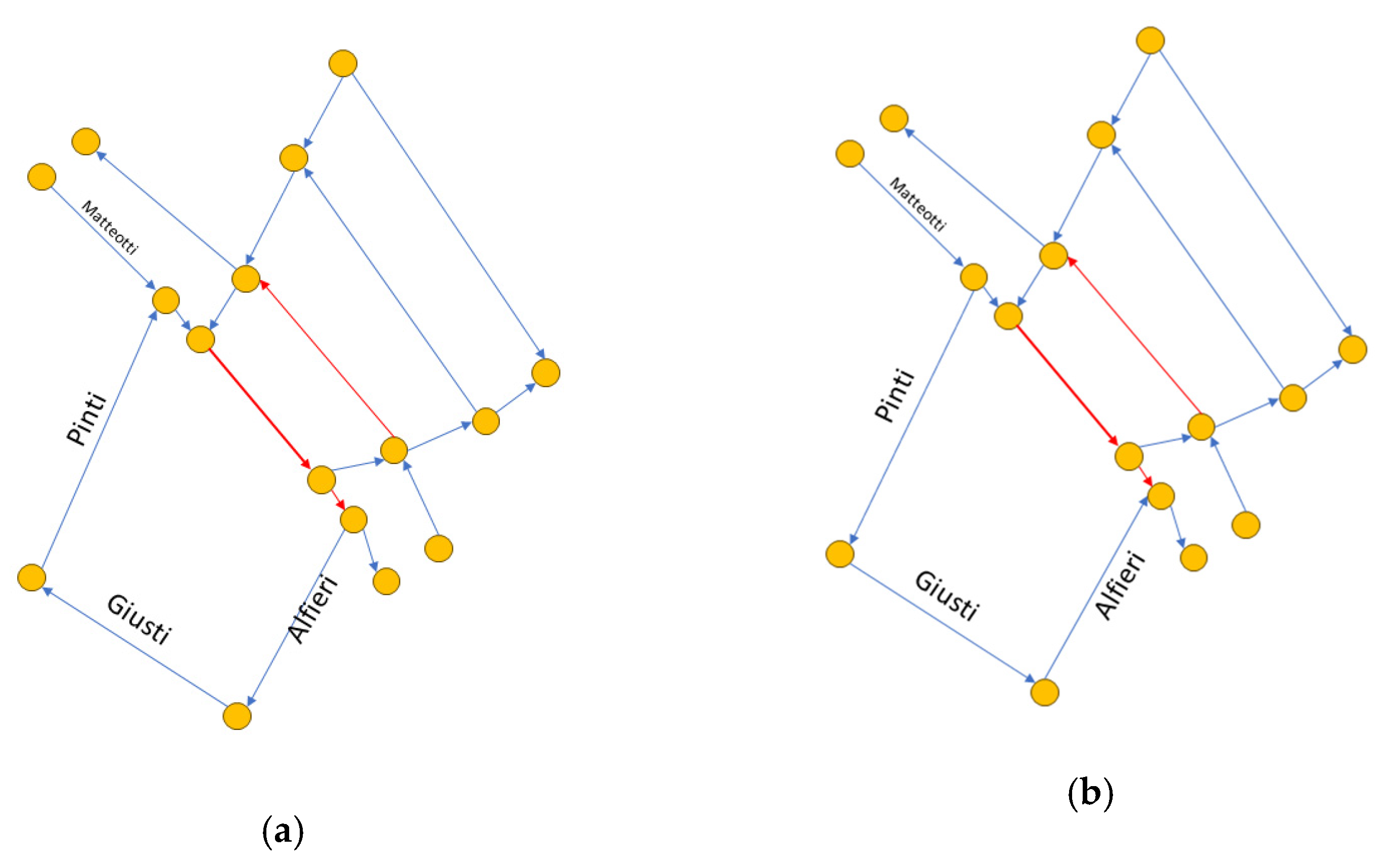
3.2. Formal Road Graph Data Model
- is the set of nodes forming the road graph (i.e., the road junctions).
- is the set of edges of the road graph, where means that there is a physical link allowing one to go from node v to node w and vice versa.
- R is the set of roads.
- is a function associating a GPS position to each node.
- is a function associating each edge to the road it belongs to.
- is a function stating for each edge the direction in which it can be traversed: means it can be traversed both ways; . Only from to ; . only from to .
- is a function associating the number of lanes (>0) for each edge.
- is a function that associates each edge with its max speed.
- models turn restrictions, where tuple means that the restriction of type applies to the edge via node to edge ; the node has to be shared between edges and , for example, restriction means that from edge , it is not possible to turn to edge .
- , the set of nodes of the compact version are a subset of the full version.
- and
- maps to the longest possible sequence of edges.
4. Scenario Editor
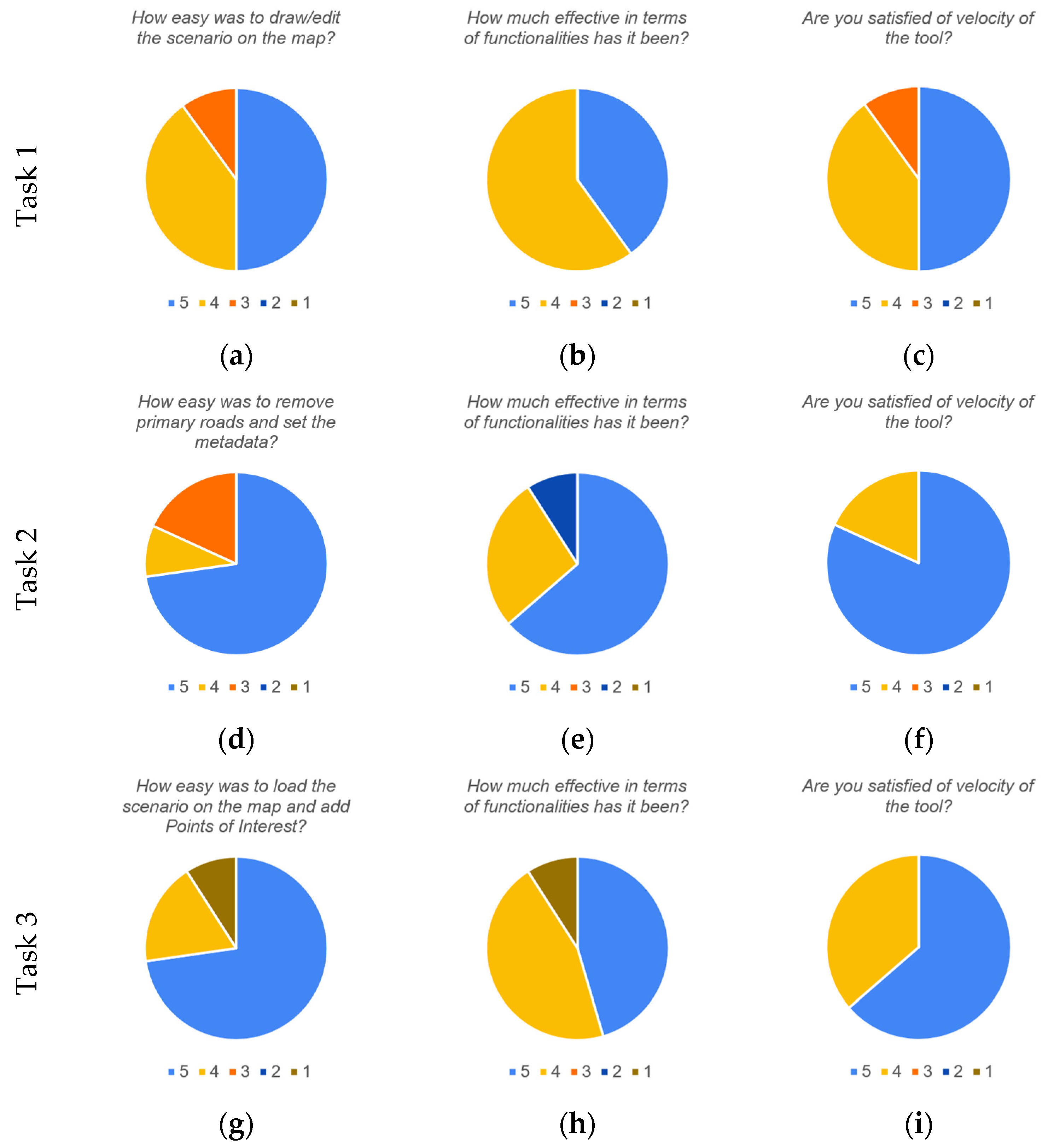
Scenario Editor Usability Test
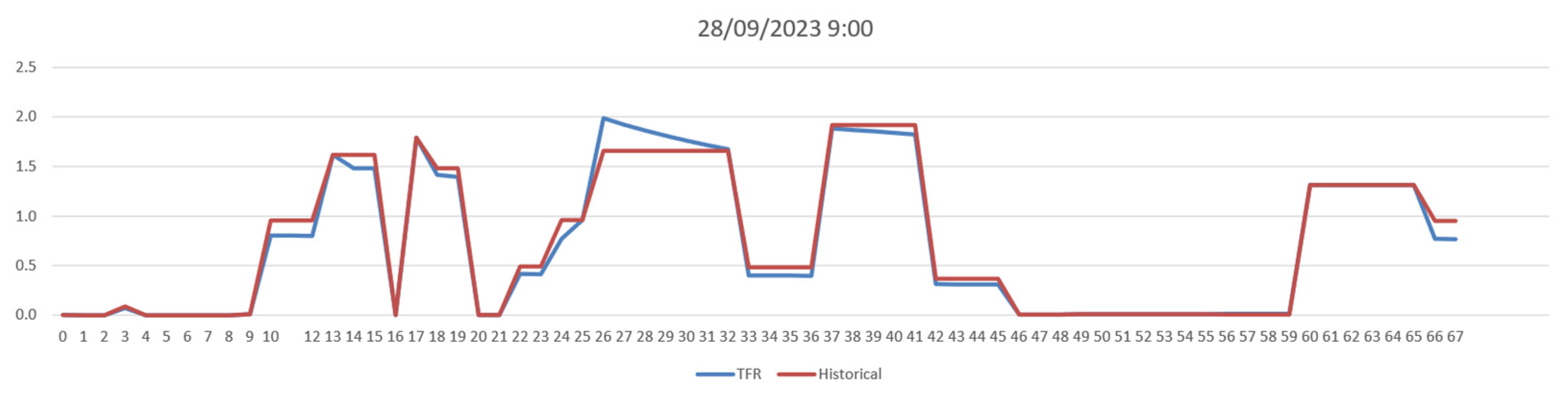
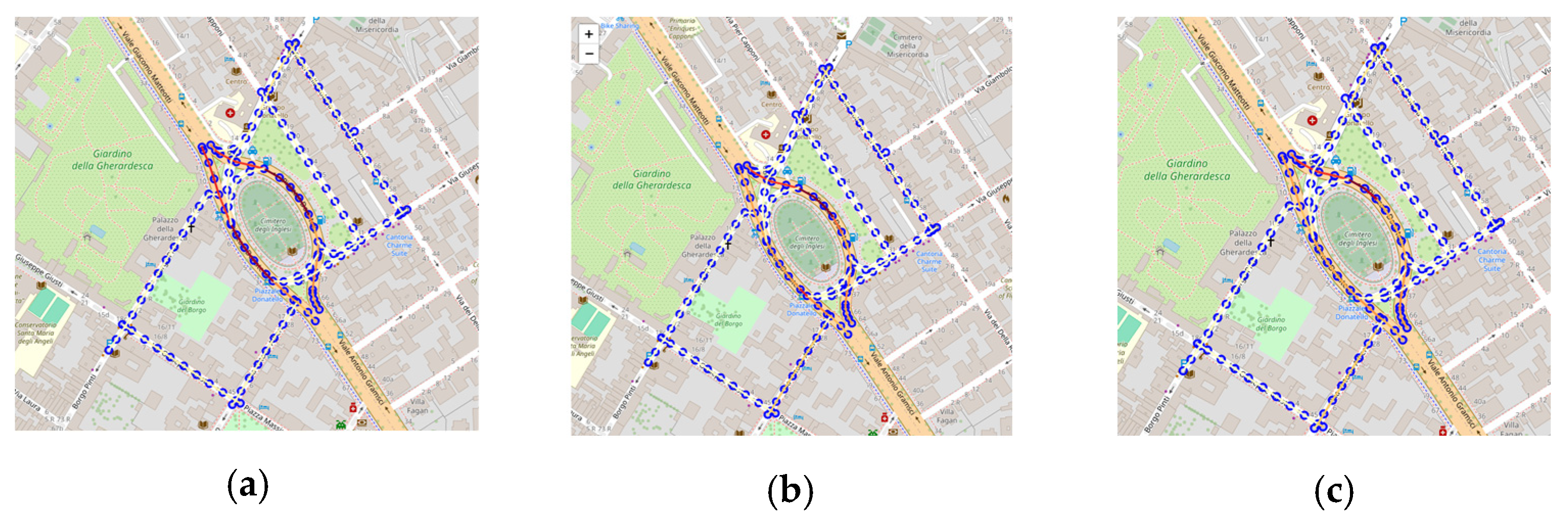
5. Case Study: Traffic Flow Reconstruction
5.1. Consistency and Correctness of TFR
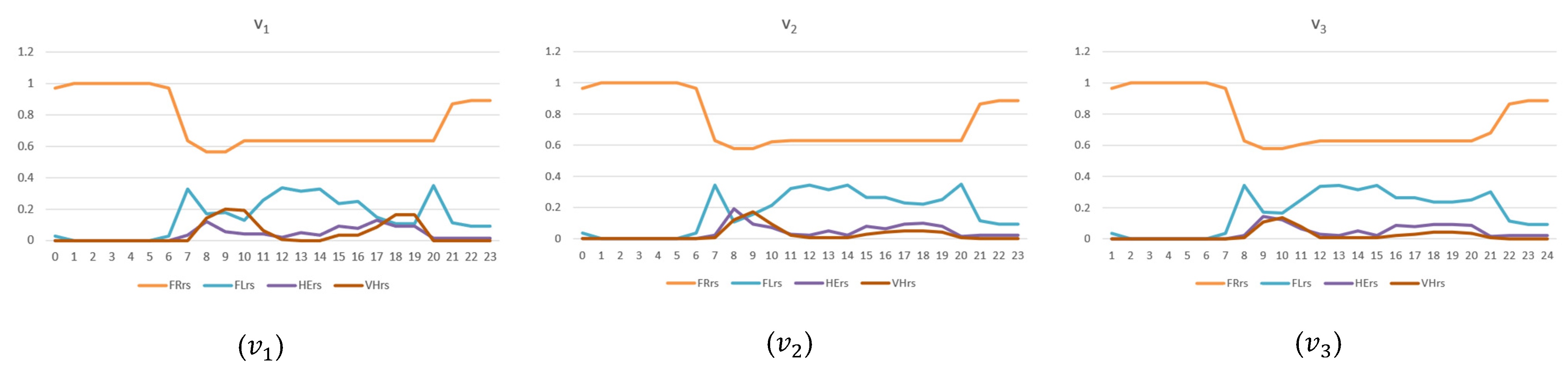
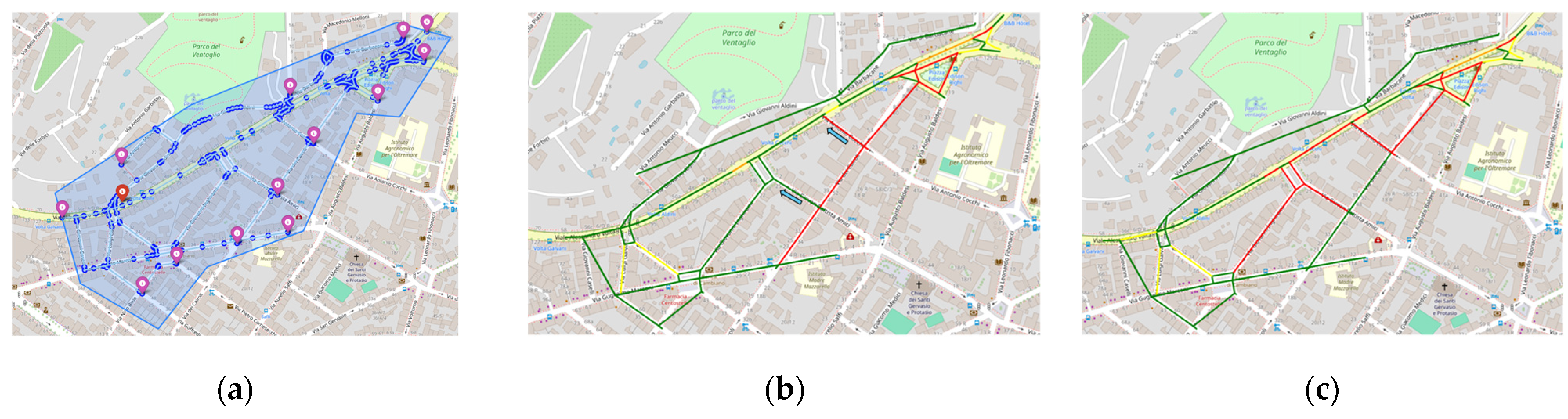
5.2. What-If Analysis for Traffic Congestion Reduction
- ,
- ,
- ,
6. Conclusions
Author Contributions
Funding
Institutional Review Board Statement
Informed Consent Statement
Data Availability Statement
Acknowledgments
Conflicts of Interest
References
- Torre-Bastida, A.I.; Del Ser, J.; Laña, I.; Ilardia, M.; Bilbao, M.N.; Campos-Cordobés, S. Big Data for transportation and mobility: Recent advances, trends and challenges. IET Intell. Transp. Syst. 2018, 12, 742–755. [Google Scholar] [CrossRef]
- Bellini, P.; Bilotta, S.; Collini, E.; Fanfani, M.; Nesi, P. Data Sources and Models for Integrated Mobility and Transport Solutions. Sensors 2024, 24, 441. [Google Scholar] [CrossRef] [PubMed]
- Hodson, M.; Marvin, S.; Robinson, B.; Swilling, M. Reshaping urban infrastructure: Material flow analysis and transitions analysis in an urban context. J. Ind. Ecol. 2012, 16, 789–800. [Google Scholar] [CrossRef]
- Keirstead, J.; Jennings, M.; Sivakumar, A. A review of urban energy system models: Approaches, challenges and opportunities. Renew. Sustain. Energy Rev. 2012, 16, 3847–3866. [Google Scholar] [CrossRef]
- Gharaibeh, A.; Salahuddin, M.A.; Hussini, S.J.; Khreishah, A.; Khalil, I.; Guizani, M.; Al-Fuqaha, A. Smart cities: A survey on data management, security, and enabling technologies. IEEE Commun. Surv. Tutor. 2017, 19, 2456–2501. [Google Scholar] [CrossRef]
- Collini, E.; Palesi LA, I.; Nesi, P.; Pantaleo, G.; Zhao, W. Flexible thermal camera solution for Smart city people detection and counting. Multimed. Tools Appl. 2023, 83, 20457–20485. [Google Scholar] [CrossRef]
- Charnes, A.; Cooper, W.W.; Li, S. Using data envelopment analysis to evaluate efficiency in the economic performance of Chinese cities. Socio-Econ. Plan. Sci. 1989, 23, 325–344. [Google Scholar] [CrossRef]
- Krylovskiy, A.; Jahn, M.; Patti, E. Designing a smart city internet of things platform with microservice architecture. In Proceedings of the 2015 3rd International Conference on Future Internet of Things and Cloud, Rome, Italy, 24–26 August 2015; pp. 25–30. [Google Scholar]
- Adreani, L.; Bellini, P.; Colombo, C.; Fanfani, M.; Nesi, P.; Pantaleo, G.; Pisanu, R. Implementing integrated digital twin modelling and representation into the Snap4City platform for smart city solutions. Multimed. Tools Appl. 2023, 1–26. [Google Scholar] [CrossRef]
- Jafari, M.; Kavousi-Fard, A.; Chen, T.; Karimi, M. A review on digital twin technology in smart grid, transportation system and smart city: Challenges and future. IEEE Access 2023, 11, 17471–17484. [Google Scholar] [CrossRef]
- Adreani, L.; Bellini, P.; Fanfani, M.; Nesi, P.; Pantaleo, G. Design and develop of a smart city digital twin with 3d representation and user interface for what-if analysis. In Proceedings of the International Conference on Computational Science and Its Applications, Athens, Greece, 3–6 July 2023; Springer Nature: Cham, Switzerland, 2023; pp. 531–548. [Google Scholar]
- Komninos, N.; Bratsas, C.; Kakderi, C.; Tsarchopoulos, P. Smart city ontologies: Improving the effectiveness of smart city applications. J. Smart Cities 2019, 1, 31–46. [Google Scholar] [CrossRef]
- Nalic, D.; Mihalj, T.; Bäumler, M.; Lehmann, M.; Eichberger, A.; Bernsteiner, S. Scenario based testing of automated driving systems: A literature survey. In Proceedings of the FISITA Web Congress, Virtual, 24 November 2020; Volume 10. [Google Scholar]
- Maierhofer, S.; Klischat, M.; Althoff, M. CommonRoad Scenario Designer: An Open-Source Toolbox for Map Conversion and Scenario Creation for Autonomous Vehicles. In Proceedings of the 2021 IEEE International Intelligent Transportation Systems Conference (ITSC), Indianapolis, IN, USA, 19–22 September 2021; pp. 3176–3182. [Google Scholar] [CrossRef]
- Kuang, L.; Gong, T.; OuYang, S.; Gao, H.; Deng, S. Offloading decision methods for multiple users with structured tasks in edge computing for smart cities. Future Gener. Comput. Syst. 2020, 105, 717–729. [Google Scholar] [CrossRef]
- Casadei, R.; Fortino, G.; Pianini, D.; Russo, W.; Savaglio, C.; Viroli, M. Modelling and simulation of opportunistic IoT services with aggregate computing. Future Gener. Comput. Syst. 2019, 91, 252–262. [Google Scholar] [CrossRef]
- Zema, N.R.; Natalizio, E.; Pugliese LD, P.; Guerriero, F. 3D Trajectory Optimization for Multimission UAVs in Smart City Scenarios. IEEE Trans. Mob. Comput. 2022, 23, 1–11. [Google Scholar] [CrossRef]
- Lohrer, A.; Binder, J.J.; Kröger, P. Group anomaly detection for spatio-temporal collective behaviour scenarios in smart cities. In Proceedings of the 15th ACM SIGSPATIAL International Workshop on Computational Transportation Science, Seattle, WA, USA, 1 November 2022; pp. 1–4. [Google Scholar]
- QGIS. Available online: https://qgis.org/ (accessed on 6 February 2024).
- ArcGIS. Available online: https://www.esri.com/en-us/arcgis/products/index (accessed on 6 February 2024).
- ASAM OpenSCENARIO. Available online: https://www.asam.net/standards/detail/openscenario-xml/ (accessed on 6 February 2024).
- ASAM OpenDRIVE. Available online: https://www.asam.net/standards/detail/opendrive/ (accessed on 6 February 2024).
- ASAM OpenCRG. Available online: https://www.asam.net/standards/detail/opencrg/ (accessed on 6 February 2024).
- OpenStreetMap iD Editor. Available online: https://github.com/openstreetmap/iD (accessed on 6 February 2024).
- SUMO, Simulation of Urban Mobility. Available online: https://eclipse.dev/sumo/ (accessed on 6 February 2024).
- PTV Vissim. Available online: https://www.ptvgroup.com/en/products/ptv-vissim (accessed on 6 February 2024).
- PTV Visum. Available online: https://www.ptvgroup.com/en/products/ptv-visum (accessed on 6 February 2024).
- SUMO Netedit Tool. Available online: https://sumo.dlr.de/docs/Netedit/ (accessed on 6 February 2024).
- FIWARE NGSIv2 (Next Generation Service Interface, Version 2) Specification. Available online: https://fiware.github.io/specifications/ngsiv2/stable/ (accessed on 6 February 2024).
- Tool Interface for Testing Scenario Editor in the Context of Many Data. Available online: https://www.snap4city.org/dashboardSmartCity/view/Baloon-Dark.php?iddasboard=MzQyMw== (accessed on 18 February 2024).
- Bellini, P.; Fanfani, M.; Nesi, P.; Pantaleo, G. Snap4city Dashboard Manager: A Tool for Creating and Distributing Complex and Interactive Dashboards with No or Low Coding. Telecommun. Eng. 2024; Preprint. [Google Scholar] [CrossRef]
- Alberti, F.; Alessandrini, A.; Bubboloni, D.; Catalano, C.; Fanfani, M.; Loda, M.; Marino, A.; Masiero, A.; Meocci, M.; Nesi, P.; et al. Mobile Mapping to Support an Integrated Transport-Territory Modelling Approach. Int. Arch.Photogramm. Remote Sens. Spat. Inf. Sci. 2023, 48, 1–7. [Google Scholar] [CrossRef]
- Bilotta, S.; Nesi, P. Traffic flow reconstruction by solving indeterminacy on traffic distribution at junctions. Future Gener. Comput. Syst. 2021, 114, 649–660. [Google Scholar] [CrossRef]
- Anagnostopoulos, T.; Zaslavsky, A.; Kolomvatsos, K.; Medvedev, A.; Amirian, P.; Morley, J.; Hadjieftymiades, S. Challenges and Opportunities of Waste Management in IoT-Enabled Smart Cities: A Survey. IEEE Trans. Sustain.Comput. 2017, 2, 275–289. [Google Scholar] [CrossRef]
- Viale Pereira, G.; Cunha, M.A.; Lampoltshammer, T.J.; Parycek, P.; Testa, M.G. Increasing collaboration and participation in smart city governance: A cross-case analysis of smart city initiatives. Inf. Technol. Dev. 2017, 23, 526–553. [Google Scholar] [CrossRef]
- Cirillo, F.; Gómez, D.; Diez, L.; Maestro, I.E.; Gilbert, T.B.J.; Akhavan, R. Smart city IoT services creation through large-scale collaboration. IEEE Internet Things J. 2020, 7, 5267–5275. [Google Scholar] [CrossRef]
- Kiba-Janiak, M.; Witkowski, J. Sustainable urban mobility plans: How do they work? Sustainability 2019, 11, 4605. [Google Scholar] [CrossRef]
- PUMS. Piano Urbano della Mobilità Sostenibile. Available online: https://www.osservatoriopums.it/ (accessed on 6 February 2024).
- SUMI. Sustainable Urban Mobility Indicators. Available online: https://trimis.ec.europa.eu/project/sustainable-urban-mobility-indicators (accessed on 6 February 2024).
- GDPR. General Data Protection Regulation. Available online: https://gdpr.eu/ (accessed on 6 February 2024).
- Snap4City Scenario Editor Usability Test. Available online: https://www.snap4city.org/dashboardSmartCity/view/index.php?iddasboard=NDE2MQ== (accessed on 11 March 2024).


| ID | Name | Description of the Functional Requirements of a Scenario Editor |
|---|---|---|
| R01 | Map visualization and controls | Show/select ground map to be used as the main canvas over which the user can define and study the scenario. Controls to move and zoom in on the map must be provided, with the possibility of changing the ground map when needed. The map is a visual representation of the geo information, for the minimal case, the graphs of roads, their relationships, and details. |
| R02 | Area of interest definition | Draw/change a polygonal shape of arbitrary size to define the area of interest of the scenario, selecting a portion of the map and of the corresponding geo information. The scenario could be composed of multiple disjoint areas. |
| R03 | Metadata setting | Set some metadata describing the scenario, such as its name, a description, the temporal validity (from date time to date time), the author, a purpose, etc. |
| R04 | Knowledge base management | Work on different maps and geo information, which can be coded into different knowledge bases or other storages, to fetch the geolocated information (i.e., entities and roads) to be taken into account in the scenario. |
| R05 | Road graph selection and management | Manage the road graph; each road segment must be visualized and managed in the scenarios. The road segments may present a number of descriptive characteristics, such as, type, travel direction, presence of restrictions, lanes, sidewalks, parking lots, etc. Each road must be selectable by the user to access additional information, such as name, type, length, number of lanes, maximum speed, etc. The manipulation of the road graph must be possible, for example, add, remove, or alter a road, invert the travel direction, increase or reduce the number of lanes, etc. In the representations of road segments, visual coding should be used to provide information at a glance. |
| R06 | Entity selection and management | Manage geolocated entities such as IoT devices with time series data (such as semaphores, sensors/actuators, waste bins, parking sensors, luminaries, Wi-Fi access points, tv cameras, parking in structures); urban furniture (such as pedestrian crossing, benches, flowerbeds, fountains for drinkable water, toilets); and POIs (such as banks, cultural services, schools, commercial areas, restaurants, hotels). They must be visualized over the map upon user request. Each entity must be selectable by the user to inspect additional information (i.e., metadata, position, real-time and/or historic data, etc.). The manipulation of entities must be permitted, for example, to disable/enable an IoT device, select the measurements of interest, choose between real-time, historic, predicted, typical time trend data, change the semaphore timings, move a pedestrian crossing, etc. |
| R07 | Enabling analytic computation | Define the context on which one could apply a large number of analytical processes including for example, the computation of traffic flow reconstructions, environmental analysis, environmental heatmaps, 15 min city index, KPIs to quantify some analysis, semaphore analysis, etc. For each analytic, the user has to be capable of composing the scenario and composing different inputs. This is the basis on which to enable the usage of the scenario for what-if analysis, exploiting several scenarios that must be inspected to verify their validity for solving a specific case. |
| R08 | Validation through the activation of consistency analysis | Validate the scenario by means of one or a set of methods to assess its consistency and completeness in terms of road graph, entities, metadata, etc. The validation process has to involve an in-depth spatial analysis of the road graph as well as the compatibility check among the selected inputs. |
| R09 | Scenario evolution over time | A scenario can evolve over time in terms of operative status (e.g., proposed, accepted, rejected), processing status (e.g., init, runnable, completed), and version. Each step must be related to a specific timestamp. |
| R10 | Scenario management | To create a new scenario, save the defined scenario, load a previously created scenario, and save it again, possibly with a different name, etc. |
| R11 | Models and custom | Scenario should be conformant to a model, on which additional variables can be added. |
| Req. | GIS [19,20] | OSM iD Editor [24] | SUMO Netedit [28] | PTV [26,27] | Snap4City |
|---|---|---|---|---|---|
| R01 | Yes | Yes | Yes (limited) | Yes (limited) | Yes |
| R02 | No | No | No | No | Yes |
| R03 | No | No | Yes | Yes | Yes |
| R04 | Yes | No | Yes | Yes | Yes |
| R05 | Yes | Yes | Yes | Yes | Yes |
| R06 | Yes (no real-time) | Yes (no real-time) | Yes (no real-time) | Yes (no real-time) | Yes |
| R07 | No | No | Yes (traffic only) | Yes (traffic only) | Yes |
| R08 | No | Yes | Yes (partial) | Yes | Yes |
| R09 | Yes (manual) | Yes (changelog) | Yes (manual) | Yes | Yes |
| R10 | Yes | Yes | Yes | Yes | Yes |
| R11 | No | Yes | Yes | Yes | Yes |
| Task | Question | AVG | STD |
|---|---|---|---|
| 1 | (a) How easy was to draw/edit the scenario on the map? | 4.4 | 0.7 |
| (b) How much effective in terms of functionalities has it been? | 4.4 | 0.5 | |
| (c) Are you satisfied with the velocity of the tool? | 4.4 | 0.7 | |
| 2 | (d) How easy was to remove primary roads and set the metadata? | 4.5 | 0.8 |
| (e) How much effective in terms of functionalities has it been? | 4.5 | 0.9 | |
| (f) Are you satisfied with the velocity of the tool? | 4.8 | 0.4 | |
| 3 | (g) How easy was to load the scenario on the map and add Points of Interest? | 4.5 | 1.2 |
| (h) How much effective in terms of functionalities has it been? | 4.2 | 1.1 | |
| (i) Are you satisfied with the velocity of the tool? | 4.6 | 0.5 |
| Scenario Version | FRrs (FreeFlow) | FLrs (FluidFlow) | HErs (HeavyFlow) | VHrs (VeryHeavyFlow) |
|---|---|---|---|---|
| 0.7649 | 0.1501 | 0.0396 | 0.0455 | |
| 0.7607 | 0.1705 | 0.0414 | 0.0274 | |
| 0.7622 | 0.1744 | 0.0411 | 0.0223 |
| Delta | Value | Percentage of Reduction |
|---|---|---|
| 0.00416 | −0.54% | |
| 0.00267 | −0.35% | |
| −0.0205 | 13.69% | |
| −0.0244 | 16.27% | |
| −0.0017 | −4.51% | |
| −0.0014 | −3.76% | |
| 0.0181 | 39.86% | |
| 0.0232 | 50.98% |
| Scenario Version | FRrs (FreeFlow) | FLrs (FluidFlow) | HErs (HeavyFlow) | VHrs (VeryHeavyFlow) |
|---|---|---|---|---|
| 0.8071 | 0.0414 | 0.0251 | 0.1264 | |
| 0.7293 | 0.0569 | 0.0174 | 0.1961 |
| Scenario Version | Computational Times (s) |
|---|---|
| 161.259 | |
| 162.330 | |
| 159.402 | |
| 120.368 | |
| 126.924 |
Disclaimer/Publisher’s Note: The statements, opinions and data contained in all publications are solely those of the individual author(s) and contributor(s) and not of MDPI and/or the editor(s). MDPI and/or the editor(s) disclaim responsibility for any injury to people or property resulting from any ideas, methods, instructions or products referred to in the content. |
© 2024 by the authors. Licensee MDPI, Basel, Switzerland. This article is an open access article distributed under the terms and conditions of the Creative Commons Attribution (CC BY) license (https://creativecommons.org/licenses/by/4.0/).
Share and Cite
Adreani, L.; Bellini, P.; Bilotta, S.; Bologna, D.; Collini, E.; Fanfani, M.; Nesi, P. Smart City Scenario Editor for General What-If Analysis. Sensors 2024, 24, 2225. https://doi.org/10.3390/s24072225
Adreani L, Bellini P, Bilotta S, Bologna D, Collini E, Fanfani M, Nesi P. Smart City Scenario Editor for General What-If Analysis. Sensors. 2024; 24(7):2225. https://doi.org/10.3390/s24072225
Chicago/Turabian StyleAdreani, Lorenzo, Pierfrancesco Bellini, Stefano Bilotta, Daniele Bologna, Enrico Collini, Marco Fanfani, and Paolo Nesi. 2024. "Smart City Scenario Editor for General What-If Analysis" Sensors 24, no. 7: 2225. https://doi.org/10.3390/s24072225
APA StyleAdreani, L., Bellini, P., Bilotta, S., Bologna, D., Collini, E., Fanfani, M., & Nesi, P. (2024). Smart City Scenario Editor for General What-If Analysis. Sensors, 24(7), 2225. https://doi.org/10.3390/s24072225