
Deep Reconstruction Transfer Convolutional Neural Network for Rolling Bearing Fault Diagnosis


Abstract
1. Introduction
- (1)
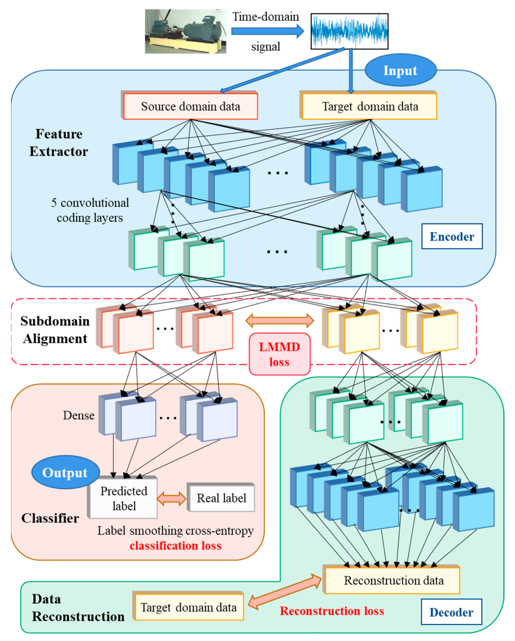
- A deep reconstruction transfer convolutional neural network (DRTCNN) is proposed. A DRTCNN is different from the existing unsupervised transfer learning in that it has a stronger ability to constrain the features of data and can deeply mine the structural information of fault signals and extract transferable features with better robustness. The DRTCNN consists of three parts: a five-layer convolutional encoder, a five-layer convolutional decoder, and a classifier considering tag confidence.
- (2)
- A five-layer shared convolutional encoder is built as a part of the source domain data feature extractor and the target domain data reconstructor. The first layer uses a wide convolutional kernel with a size of 1 × 64 to effectively filter the noise in the high frequency band and capture the impact of the bearing. Using a shared coding representation to alternately learn source domain label prediction and target domain data reconstruction is helpful for the network to better extract the domain invariant features of the two domains. The signal reconstructor, constructed by a five-layer decoder and five-layer encoder, is used to reconstruct the target domain data and can fully mine the available structure information from the untagged original signal.
- (3)
- The smooth label, cross-entropy loss assistant training classifier is introduced to consider the confidence of the sample label, reduce the impact of dataset error tags, and prevent model overfitting.
- (4)
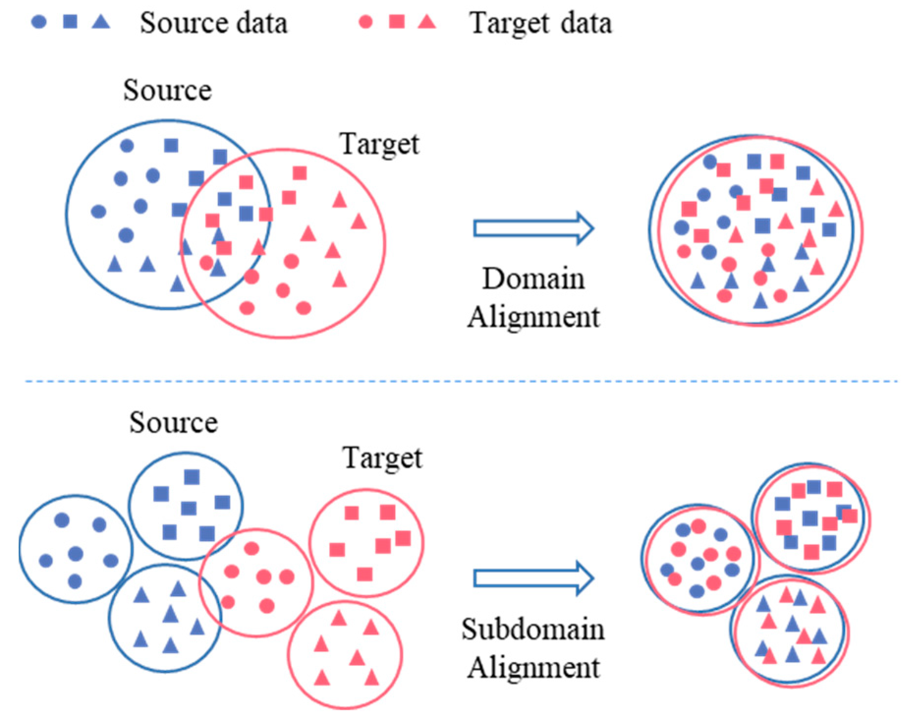
- A new subdomain adaptive function is introduced, which is called the local maximum mean discrepancy (LMMD) algorithm. Combined with the proposed DRTCNN, the algorithm maps the source domain and target domain data to the same potential space, minimizes the domain offset of each subdomain, and realizes the alignment between the source domain subdomain and the target domain subdomain.
- (5)
- Through the CWRU dataset, BJTU dataset, and SEU dataset, 20 transfer experiments are carried out, and the diagnostic effect of the DRTCNN is compared with the existing transfer learning network to verify the superiority of the structure proposed in this paper. Through the ablation experiment, the effectiveness of each component of the network is verified, and the optimal selection of key dynamic tradeoff factors is discussed and analyzed.
2. Convolutional Autoencoder Neural Network
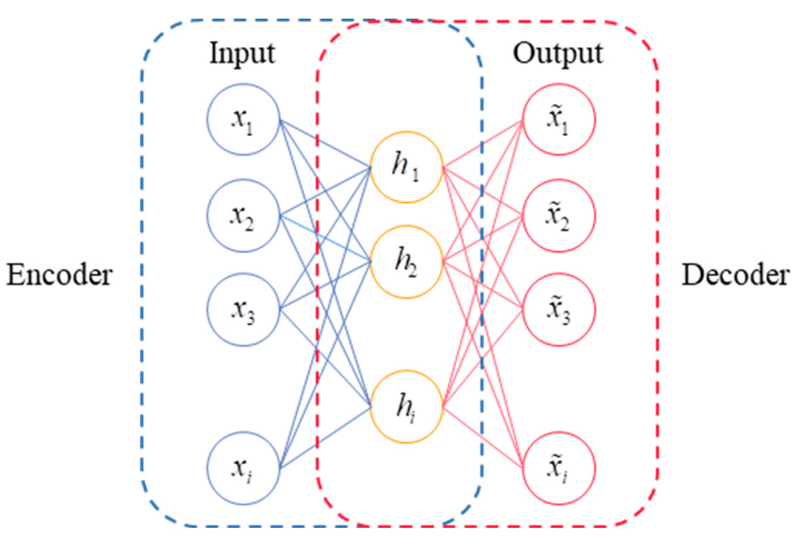
2.1. Autoencoder Structure
2.2. Design of Basic Convolutional Self-Coding Network Model
3. Deep Reconstructed Convolution Network
3.1. Unsupervised Auxiliary Training Based on Signal Reconstruction
3.2. Domain Alignment Optimization Based on Distance
3.3. Training Optimization Based on Label Smoothing
3.4. Loss Function Considering Dynamic Trade-Off
3.5. Method Flow of Fault Diagnosis across Working Conditions
- (1)
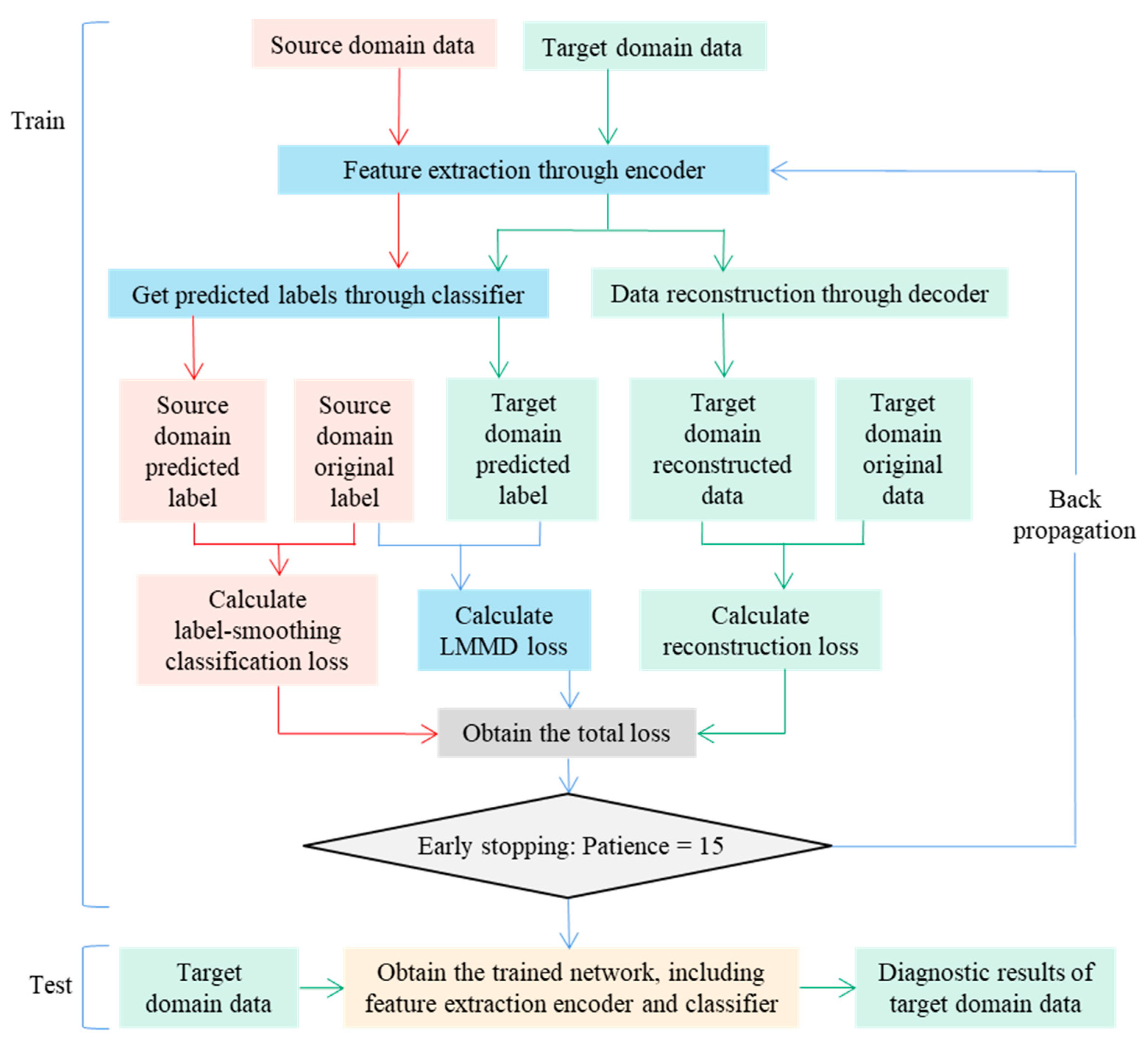
- Input data: The labeled source domain training set and the unlabeled target domain training set are entered, the dynamic trade-off factor γ, the maximum training time E, and the number of early stops s are set, and the parameter set θ to be trained is randomly initialized.
- (2)
- Forward propagation: The encoder composed of five-layer convolutional blocks extracts the transferable features hs and ht of the source domain and the target domain. The prediction labels and of the source domain and the target domain are obtained from the full connection layer and the softmax function, the prediction labels of the source domain and the target domain are obtained, and the prediction labels of the source domain and the target domain are used to calculate the cross-entropy loss of the smooth label. The classification loss of the samples in the source domain is obtained using Expression (18). The classification loss is obtained by using the execution in the LMMD algorithm. The distribution distance of the same label subdomain between the source domain and the target domain is calculated using Expression (12), and is obtained. At the same time, the target domain signal feature ht, which is extracted by the encoder, is reconstructed by the decoder, the reconstructed signal is obtained using Expression (6), and the reconstruction loss of the target domain data is calculated using Expression (7). When the patience of early stopping reaches 15, step (4) is performed; otherwise, step (3) is performed.
- (3)
- Back propagation: The Adam optimizer is selected, and the total loss value is obtained from expression (19) and backpropagated. After updating the parameter set θ to be trained, step (2) is performed.
- (4)
- Test model: The target domain test set data are inputted into the model, go through the encoder feature extraction module and the fully connected classification module, and the final output label is the diagnosis result of the target domain data.
4. Experimental Verification of Rolling Bearing Fault Diagnosis
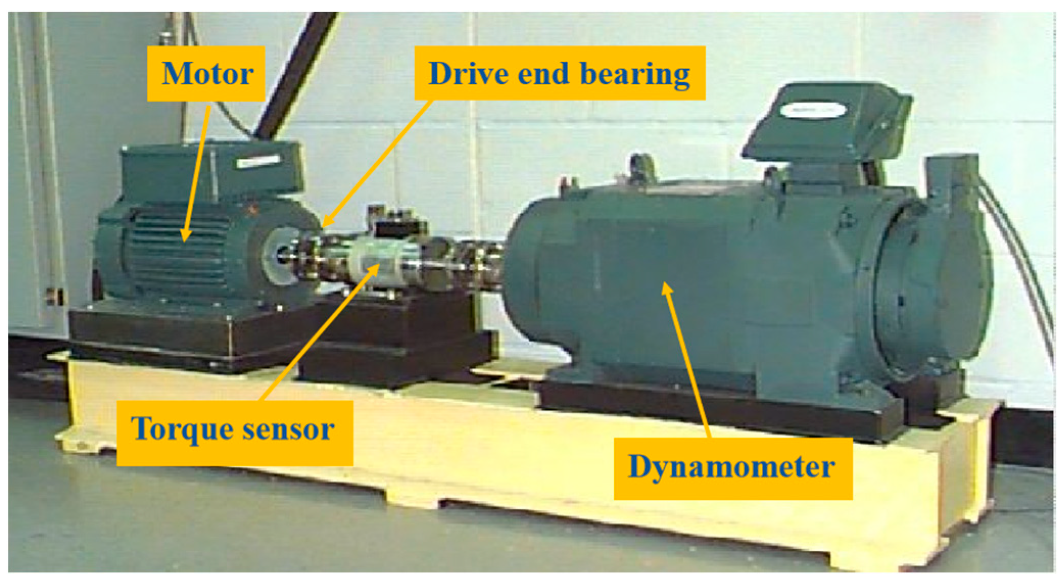
4.1. Introduction of Fault Dataset
4.2. Comparative Study and Design of Models
- (1)
- DCTLN: the conditional recognition network is constructed using a six-layer CNN, and the MMD algorithm is used to maximize the domain recognition error and minimize the probability distribution distance to complete the transfer.
- (2)
- FTNN: the transferable features are extracted using a two-layer, small convolution kernel CNN, and the domain adaptation is realized by multi-layer domain adaptation and pseudo-label learning through an MMD algorithm.
- (3)
- DASAN: the feature extractor is constructed using a three-layer, small convolution kernel CNN, and the global domain adaptation and subdomain adaptation are realized by combining the LMMD algorithm.
- (4)
- DNCNN: two layers of the CNN are used as the feature extraction layer, and the size of the convolution kernel is 15.
- (5)
- DAHAN: two layers of a wide convolution kernel CNN are used to extract signal features; the first layer uses a wide convolution kernel with a size of 128, and the second layer uses a slightly smaller wide convolution kernel with a size of 64.
- (6)
- MWDAN: the feature extraction part consists of four layers of a CNN: the first layer is wide convolution, and the convolution kernel size is 64; the other convolution layers use a small convolution kernel, where the size is [16, 5, 5].
4.3. Experimental Results and Discussion
4.3.1. Analysis of Experimental Results of Fault Diagnosis across Different Working Conditions
4.3.2. Ablation Experiment and Results Analysis
- (1)
- M1: the local maximum mean difference module is deleted, the subdomains of the source domain and the target domain are no longer aligned in the training process, and the returned loss function only has two parts: classification loss and reconstruction loss.
- (2)
- M2: the decoder module is deleted; that is, the target domain signal is no longer reconstructed, and the loss function consists of two parts: classification loss and LMMD loss; the training of model parameters is only related to data classification and subdomain alignment.
- (3)
- M3: the local maximum mean difference module and the decoder module are deleted at the same time, and the returned loss value is only the classification loss.
- (4)
- M4: the smooth label processing is deleted, the basic cross-entropy loss is used as the classification loss function, and the LMMD loss and reconstruction loss are retained.
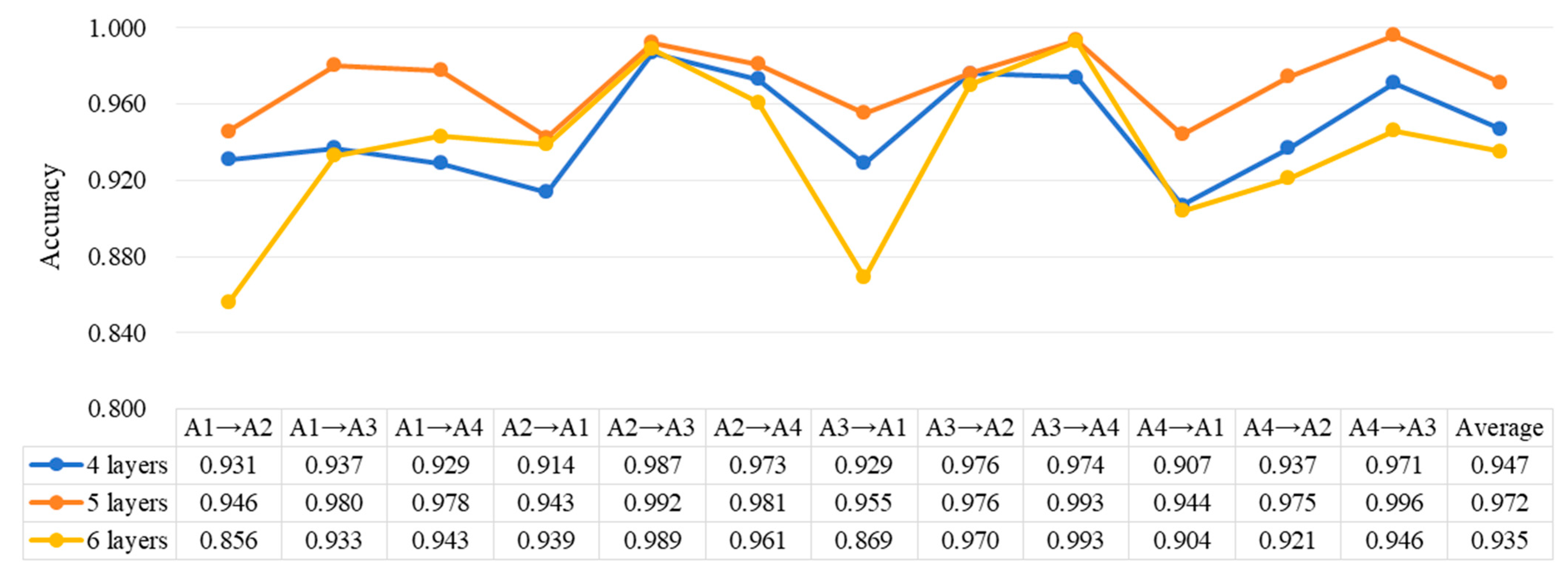
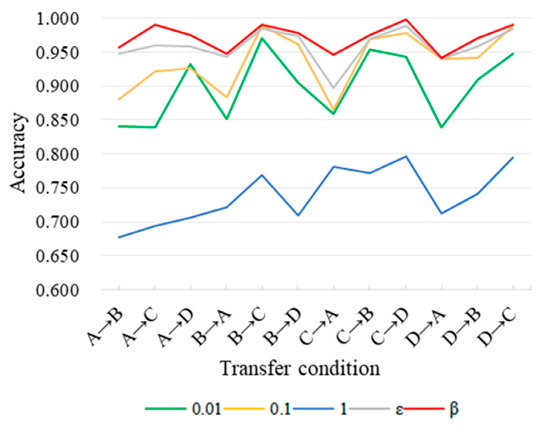
4.3.3. Comparative Analysis of Network Structure and Key Parameters
5. Conclusions
- (1)
- The hidden features in the original signal are extracted using the deep reconstruction and transfer network, and combined with a new subdomain alignment algorithm to expand the inter-class distance and reduce the intra-class distance. It is helpful to construct the generalized decision boundary, reduce the influence of the change in working conditions on fault mapping, and effectively improve the recognition accuracy of the model in cross-domain fault diagnosis tasks. In the process of signal reconstruction, the decoder makes full use of the structure information of the target domain data and fully mines the domain invariant features.
- (2)
- Through the construction of a five-layer deep convolution self-encoder with a wide kernel in the first layer, the function of adaptive noise reduction is realized, which does not depend on noise reduction preprocessing and has stronger data feature constraint ability.
- (3)
- In the process of model training, the cross-entropy loss of smooth tags considering confidence is introduced to reduce the trust of wrong tags in the training process, restrain the overfitting of the model, and enhance the effectiveness of feature learning of the network.
- (4)
- Through the verification of 20 transfer tasks constructed by three rolling bearing fault datasets, compared with the existing transfer learning network, the proposed DRTCNN achieves a better fault identification accuracy and generalization performance in the target working conditions and noise environment.
Author Contributions
Funding
Institutional Review Board Statement
Informed Consent Statement
Data Availability Statement
Acknowledgments
Conflicts of Interest
References
- Liu, Q.; Wang, Y.; Xu, Y. Synchrosqueezing extracting transform and its application in bearing fault diagnosis under non-stationary conditions. Measurement 2021, 173, 108569. [Google Scholar] [CrossRef]
- He, K.; Zhang, X.; Ren, S.; Sun, J. Deep Residual Learning for Image Recognition. In Proceedings of the 2016 IEEE Conference on Computer Vision and Pattern Recognition (CVPR), Las Vegas, NV, USA, 27–30 June 2016; IEEE: New York, NY, USA, 2016. [Google Scholar]
- Wei, Y.; Li, Y.; Xu, M.; Huang, W. A Review of Early Fault Diagnosis Approaches and Their Applications in Rotating Machinery. Entropy 2019, 21, 409. [Google Scholar] [CrossRef]
- Wang, H.; Li, C.; Du, W. Coupled Hidden Markov Fusion of Multichannel Fast Spectral Coherence Features for Intelligent Fault Diagnosis of Rolling Element Bearings. IEEE Trans. Instrum. Meas. 2021, 70, 1–10. [Google Scholar] [CrossRef]
- Guo, Y.; Yang, D.; Zhang, Y.; Wang, L.; Wang, K. Online estimation of SOH for lithium-ion battery based on SSA-Elman neural network. Prot. Control Mod. Power Syst. 2022, 7, 1–17. [Google Scholar] [CrossRef]
- Shao, X.; Kim, C.-S. Unsupervised Domain Adaptive 1D-CNN for Fault Diagnosis of Bearing. Sensors 2022, 22, 4156. [Google Scholar] [CrossRef]
- Abdeljaber, O.; Avci, O.; Kiranyaz, S.; Gabbouj, M.; Inman, D.J. Real-time vibration-based structural damage detection using one-dimensional convolutional neural networks. J. Sound Vib. 2017, 388, 154–170. [Google Scholar] [CrossRef]
- Chen, X.; Zhang, B.; Gao, D. Bearing fault diagnosis base on multi-scale CNN and LSTM model. J. Intell. Manuf. 2021, 32, 971–987. [Google Scholar] [CrossRef]
- Ozcan, I.H.; Devecioglu, O.C.; Ince, T.; Eren, L.; Askar, M. Enhanced bearing fault detection using multichannel, multilevel 1D CNN classifier. Electr. Eng. 2022, 104, 435–447. [Google Scholar] [CrossRef]
- He, J.; Yang, S.; Gan, C. Unsupervised Fault Diagnosis of a Gear Transmission Chain Using a Deep Belief Network. Sensors 2017, 17, 1564. [Google Scholar] [CrossRef] [PubMed]
- Zhu, J.; Hu, T.; Jiang, B.; Yang, X. Intelligent bearing fault diagnosis using PCA–DBN framework. Neural Comput. Appl. 2019, 32, 10773–10781. [Google Scholar] [CrossRef]
- Shao, H.; Jiang, H.; Wang, F.; Wang, Y. Rolling bearing fault diagnosis using adaptive deep belief network with dual-tree complex wavelet packet. ISA Trans. 2017, 69, 187–201. [Google Scholar] [CrossRef]
- Hinton, G.E.; Salakhutdinov, R.R. Reducing the Dimensionality of Data with Neural Networks. Science 2006, 313, 504–507. [Google Scholar] [CrossRef]
- Wang, J.; Jiang, X.; Li, S.; Xin, Y. A novel feature representation method based on deep neural networks for gear fault diagnosis. In Proceedings of the 2017 Prognostics and System Health Management Conference (PHM-Harbin), Harbin, China, 9–12 July 2017; IEEE: New York, NK, USA, 2017. [Google Scholar]
- Sun, J.; Yan, C.; Wen, J. Intelligent Bearing Fault Diagnosis Method Combining Compressed Data Acquisition and Deep Learning. IEEE Trans. Instrum. Meas. 2018, 67, 185–195. [Google Scholar] [CrossRef]
- Li, Y.; Zeng, Y.; Qing, Y.; Huang, G.-B. Learning local discriminative representations via extreme learning machine for machine fault diagnosis. Neurocomputing 2020, 409, 275–285. [Google Scholar] [CrossRef]
- Guo, L.; Lei, Y.; Xing, S.; Yan, T.; Li, N. Deep Convolutional Transfer Learning Network: A New Method for Intelligent Fault Diagnosis of Machines With Unlabeled Data. IEEE Trans. Ind. Electron. 2019, 66, 7316–7325. [Google Scholar] [CrossRef]
- Yang, B.; Lei, Y.; Jia, F.; Xing, S. An intelligent fault diagnosis approach based on transfer learning from laboratory bearings to locomotive bearings. Mech. Syst. Signal Process. 2019, 122, 692–706. [Google Scholar] [CrossRef]
- Liu, Y.; Wang, Y.; Chow, T.W.S.; Li, B. Deep Adversarial Subdomain Adaptation Network for Intelligent Fault Diagnosis. IEEE Trans. Ind. Inform. 2022, 18, 6038–6046. [Google Scholar] [CrossRef]
- Jia, F.; Lei, Y.; Lu, N.; Xing, S. Deep normalized convolutional neural network for imbalanced fault classification of machinery and its understanding via visualization. Mech. Syst. Signal Process. 2018, 110, 349–367. [Google Scholar] [CrossRef]
- Yang, B.; Wang, T.; Xie, J.; Yang, J. Deep Adversarial Hybrid Domain-Adaptation Network for Varying Working Conditions Fault Diagnosis of High-Speed Train Bogie. IEEE Trans. Instrum. Meas. 2023, 72, 3517510. [Google Scholar] [CrossRef]
- Cheng, C.; Zhou, B.; Ma, G.; Wu, D.; Yuan, Y. Wasserstein distance based deep adversarial transfer learning for intelligent fault diagnosis with unlabeled or insufficient labeled data. Neurocomputing 2020, 409, 35–45. [Google Scholar] [CrossRef]
- Chen, P.; Zhao, R.; He, T.; Wei, K.; Yang, Q. Unsupervised domain adaptation of bearing fault diagnosis based on Join Sliced Wasserstein Distance. ISA Trans. 2022, 129, 504–519. [Google Scholar] [CrossRef] [PubMed]
- Wang, X. A method for estimating the healthy operation state of 110kV power grid transformers based on key characteristic quantities. In Proceedings of the Second International Conference on Testing Technology and Automation Engineering (TTAE 2022), Changchun, China, 26–28 August 2022; SPIE: Bellingham, WA, USA, 2022. [Google Scholar]
- Ganin, Y.; Ustinova, E.; Ajakan, H.; Germain, P.; Larochelle, H.; Laviolette, F.; Marchand, M.; Lempitsky, V. Domain-Adversarial Training of Neural Networks. In Domain Adaptation in Computer Vision Applications; Csurka, G., Ed.; Springer International Publishing: Cham, Switzerland, 2017; pp. 189–209. [Google Scholar]
- Han, T.; Liu, C.; Yang, W.; Jiang, D. A novel adversarial learning framework in deep convolutional neural network for intelligent diagnosis of mechanical faults. Knowl.-Based Syst. 2019, 165, 474–487. [Google Scholar] [CrossRef]
- Jiao, J.; Zhao, M.; Lin, J. Unsupervised Adversarial Adaptation Network for Intelligent Fault Diagnosis. IEEE Trans. Ind. Electron. 2020, 67, 9904–9913. [Google Scholar] [CrossRef]
- Jiao, J.; Zhao, M.; Lin, J. Multi-Weight Domain Adversarial Network for Partial-Set Transfer Diagnosis. IEEE Trans. Ind. Electron. 2022, 69, 4275–4284. [Google Scholar] [CrossRef]
- Zhang, W.; Peng, G.; Li, C.; Chen, Y.; Zhang, Z. A New Deep Learning Model for Fault Diagnosis with Good Anti-Noise and Domain Adaptation Ability on Raw Vibration Signals. Sensors 2017, 17, 425. [Google Scholar] [CrossRef]
- Gretton, A.; Borgwardt, K.M.; Rasch, M.J.; Schölkopf, B.; Smola, A. A kernel two-sample test. J. Mach. Learn. Res. 2012, 13, 723–773. [Google Scholar]
- Long, M.S.; Zhu, H.; Wang, J.M.; Jordan, M. Deep Transfer Learning with Joint Adaptation Networks. In Proceedings of the 34th International Conference on Machine Learning, Sydney, Australia, 6–11 August 2017. [Google Scholar]
- Long, M.S.; Cao, Y.; Wang, J.M.; Jordan, M.I. Learning Transferable Features with Deep Adaptation Networks, 32nd. In Proceedings of the International Conference on Machine Learning, Lille, France, 7–9 July 2015; pp. 97–105. [Google Scholar]
- Zhu, Y.; Zhuang, F.; Wang, D. Aligning Domain-Specific Distribution and Classifier for Cross-Domain Classification from Multiple Sources. In Proceedings of the AAAI Conference on Artificial Intelligence, Honolulu, HI, USA, 27 January–1 February 2019; Volume 33, pp. 5989–5996. [Google Scholar]
- Zhu, Z.; Lei, Y.; Qi, G.; Chai, Y.; Mazur, N.; An, Y.; Huang, X. A review of the application of deep learning in intelligent fault diagnosis of rotating machinery. Measurement 2023, 206, 112346. [Google Scholar] [CrossRef]
- Szegedy, C.; Vanhoucke, V.; Ioffe, S.; Shlens, J.; Wojna, Z. Rethinking the Inception Architecture for Computer Vision. In Proceedings of the 2016 IEEE Conference on Computer Vision and Pattern Recognition (CVPR), Las Vegas, NV, USA, 27–30 June 2016; IEEE: New York, NK, USA, 2016. [Google Scholar]


| Layer Type | Kernel Size | Stride | Kernel Channel Size |
|---|---|---|---|
| Convolution 1 | 64 × 1 | 16 × 1 | 16 |
| Pooling 1 | 2 × 1 | 2 × 1 | 16 |
| Convolution 2 | 3 × 1 | 1 × 1 | 32 |
| Pooling 2 | 2 × 1 | 2 × 1 | 32 |
| Convolution 3 | 3 × 1 | 1 × 1 | 64 |
| Pooling 3 | 2 × 1 | 2 × 1 | 64 |
| Convolution 4 | 3 × 1 | 1 × 1 | 64 |
| Pooling 4 | 2 × 1 | 2 × 1 | 64 |
| Convolution 5 | 3 × 1 | 1 × 1 | 64 |
| Pooling 5 | 2 × 1 | 2 × 1 | 64 |
| Fully connected | 128 | 1 | |
| Softmax | Number of classes | 1 | |
| Layer Type | Kernel Size | Stride | Kernel Channel Size |
|---|---|---|---|
| Deconvolution 1 | 3 × 1 | 1 × 1 | 64 |
| Upsampling 1 | 2 × 1 | 2 × 1 | 64 |
| Deconvolution 2 | 3 × 1 | 1 × 1 | 64 |
| Upsampling 2 | 2 × 1 | 2 × 1 | 64 |
| Deconvolution 3 | 3 × 1 | 1 × 1 | 32 |
| Upsampling 3 | 2 × 1 | 2 × 1 | 32 |
| Deconvolution 4 | 3 × 1 | 1 × 1 | 16 |
| Upsampling 4 | 2 × 1 | 2 × 1 | 16 |
| Deconvolution 5 | 64 × 1 | 16 × 1 | 1 |
| Upsampling 5 | 2 × 1 | 2 × 1 | 1 |
| Fault Location | Class | Fault Diameter | Fault Depth |
|---|---|---|---|
| Inner Raceway | IRF007 | 0.007 inches | 0.011 inches |
| IRF014 | 0.014 inches | ||
| IRF021 | 0.021 inches | ||
| Outer Raceway | ORF007 | 0.007 inches | |
| ORF014 | 0.014 inches | ||
| ORF021 | 0.021 inches | ||
| Ball | BF007 | 0.007 inches | |
| BF014 | 0.014 inches | ||
| BF021 | 0.021 inches |
| Name | Class | Condition |
|---|---|---|
| A1 | BF007, BF014, BF021, IRF007, IRF014, IRF021, ORF007, ORF014, ORF021, normal | 1797 r/min, 0 HP |
| A2 | 1772 r/min, 1 HP | |
| A3 | 1750 r/min, 2 HP | |
| A4 | 1730 r/min, 3 HP | |
| B1 | Normal, ball, inner, outer | 2765 RPM, 150 km/h |
| B2 | 4400 RPM, 250 km/h | |
| B3 | 5270 RPM, 300 km/h | |
| C1 | Normal, ball, inner, outer | 20 Hz, 0 V |
| C2 | 30 Hz, 2 V |
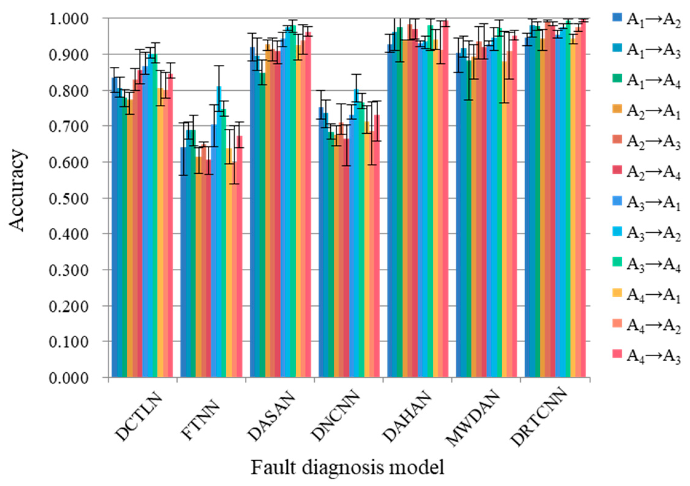
| Method | DCTLN | FTNN | DASAN | DNCNN | DAHAN | MWDAN | DRTCNN |
|---|---|---|---|---|---|---|---|
| A1→A2 | 0.835 | 0.640 | 0.921 | 0.753 | 0.926 | 0.904 | 0.946 |
| A1→A3 | 0.805 | 0.687 | 0.897 | 0.737 | 0.963 | 0.916 | 0.980 |
| A1→A4 | 0.779 | 0.688 | 0.848 | 0.683 | 0.976 | 0.883 | 0.978 |
| A2→A1 | 0.773 | 0.614 | 0.927 | 0.675 | 0.939 | 0.894 | 0.943 |
| A2→A3 | 0.830 | 0.648 | 0.914 | 0.711 | 0.983 | 0.934 | 0.992 |
| A2→A4 | 0.857 | 0.605 | 0.908 | 0.664 | 0.971 | 0.921 | 0.981 |
| A3→A1 | 0.867 | 0.704 | 0.943 | 0.730 | 0.929 | 0.927 | 0.955 |
| A3→A2 | 0.901 | 0.810 | 0.975 | 0.803 | 0.934 | 0.945 | 0.976 |
| A3→A4 | 0.902 | 0.747 | 0.981 | 0.765 | 0.980 | 0.973 | 0.993 |
| A4→A1 | 0.806 | 0.637 | 0.924 | 0.712 | 0.941 | 0.879 | 0.944 |
| A4→A2 | 0.800 | 0.599 | 0.939 | 0.687 | 0.912 | 0.910 | 0.975 |
| A4→A3 | 0.845 | 0.672 | 0.963 | 0.732 | 0.995 | 0.951 | 0.996 |
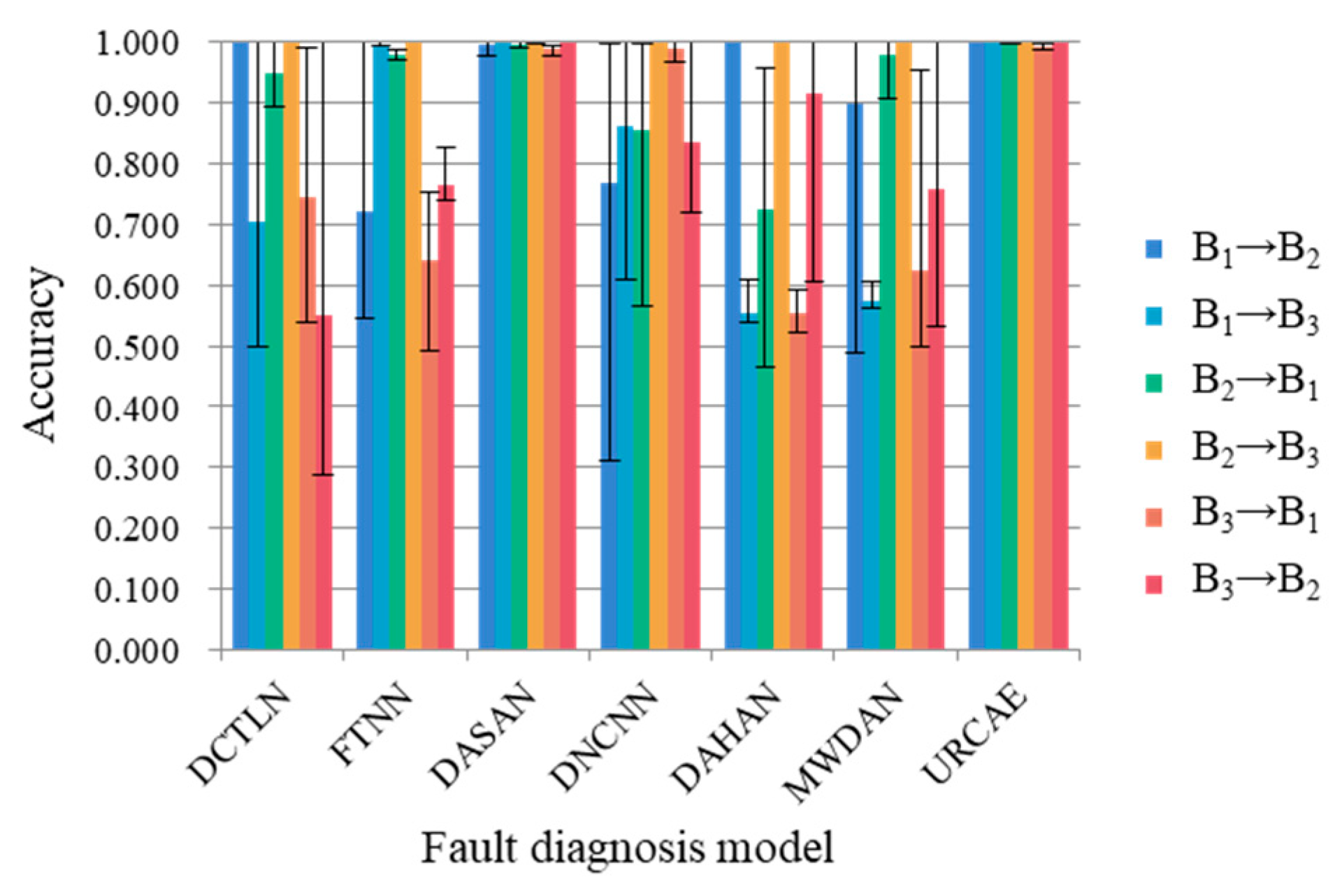
| Method | DCTLN | FTNN | DASAN | DNCNN | DAHAN | MWDAN | DRTCNN |
|---|---|---|---|---|---|---|---|
| B1→B2 | 1.000 | 0.722 | 0.995 | 0.770 | 1.000 | 0.898 | 1.000 |
| B1→B3 | 0.706 | 0.998 | 1.000 | 0.861 | 0.555 | 0.575 | 1.000 |
| B2→B1 | 0.949 | 0.978 | 0.997 | 0.857 | 0.726 | 0.980 | 0.999 |
| B2→B3 | 1.000 | 1.000 | 0.999 | 1.000 | 1.000 | 1.000 | 1.000 |
| B3→B1 | 0.747 | 0.641 | 0.989 | 0.990 | 0.554 | 0.623 | 0.993 |
| B3→B2 | 0.550 | 0.764 | 1.000 | 0.835 | 0.916 | 0.760 | 1.000 |
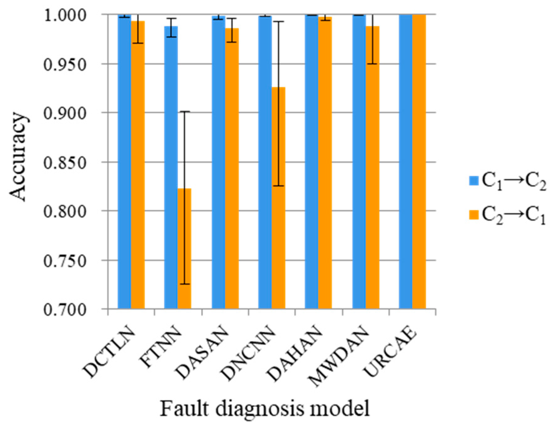
| Method | DCTLN | FTNN | DASAN | DNCNN | DAHAN | MWDAN | DRTCNN |
|---|---|---|---|---|---|---|---|
| C1→C2 | 1.000 | 0.989 | 0.999 | 0.999 | 1.000 | 1.000 | 1.000 |
| C2→C1 | 0.994 | 0.823 | 0.986 | 0.926 | 0.998 | 0.989 | 1.000 |
| Method | M1 | M2 | M3 | M4 | DRTCNN |
|---|---|---|---|---|---|
| A1→A2 | 0.864 | 0.950 | 0.847 | 0.957 | 0.960 |
| A1→A3 | 0.853 | 0.976 | 0.836 | 0.944 | 0.990 |
| A1→A4 | 0.833 | 0.971 | 0.829 | 0.943 | 0.976 |
| A2→A1 | 0.861 | 0.944 | 0.857 | 0.920 | 0.949 |
| A2→A3 | 0.977 | 0.989 | 0.974 | 0.986 | 0.990 |
| A2→A4 | 0.910 | 0.969 | 0.904 | 0.970 | 0.979 |
| A3→A1 | 0.867 | 0.917 | 0.853 | 0.920 | 0.946 |
| A3→A2 | 0.963 | 0.969 | 0.947 | 0.957 | 0.976 |
| A3→A4 | 0.956 | 0.997 | 0.951 | 0.981 | 0.999 |
| A4→A1 | 0.846 | 0.927 | 0.824 | 0.923 | 0.941 |
| A4→A2 | 0.903 | 0.976 | 0.897 | 0.930 | 0.971 |
| A4→A3 | 0.939 | 0.986 | 0.921 | 0.976 | 0.990 |
| Avg. | 0.898 | 0.964 | 0.887 | 0.951 | 0.972 |
| Method | M1 | M2 | M3 | M4 | DRTCNN |
|---|---|---|---|---|---|
| B1→B2 | 0.708 | 1.000 | 0.697 | 1.000 | 1.000 |
| B1→B3 | 1.000 | 0.508 | 0.890 | 0.508 | 1.000 |
| B2→B1 | 0.764 | 1.000 | 0.644 | 1.000 | 1.000 |
| B2→B3 | 1.000 | 1.000 | 0.782 | 1.000 | 1.000 |
| B3→B1 | 0.750 | 0.982 | 0.513 | 0.994 | 0.998 |
| B3→B2 | 0.728 | 1.000 | 0.725 | 0.995 | 1.000 |
| Avg. | 0.825 | 0.915 | 0.708 | 0.916 | 1.000 |
| Method | M1 | M2 | M3 | M4 | DRTCNN |
|---|---|---|---|---|---|
| C1→C2 | 0.981 | 0.736 | 0.976 | 0.738 | 1.000 |
| C2→C1 | 0.747 | 0.994 | 0.731 | 0.988 | 0.999 |
| Avg. | 0.864 | 0.865 | 0.853 | 0.863 | 1.000 |
Disclaimer/Publisher’s Note: The statements, opinions and data contained in all publications are solely those of the individual author(s) and contributor(s) and not of MDPI and/or the editor(s). MDPI and/or the editor(s) disclaim responsibility for any injury to people or property resulting from any ideas, methods, instructions or products referred to in the content. |
© 2024 by the authors. Licensee MDPI, Basel, Switzerland. This article is an open access article distributed under the terms and conditions of the Creative Commons Attribution (CC BY) license (https://creativecommons.org/licenses/by/4.0/).
Share and Cite
Feng, Z.; Tong, Q.; Jiang, X.; Lu, F.; Du, X.; Xu, J.; Huo, J. Deep Reconstruction Transfer Convolutional Neural Network for Rolling Bearing Fault Diagnosis. Sensors 2024, 24, 2079. https://doi.org/10.3390/s24072079
Feng Z, Tong Q, Jiang X, Lu F, Du X, Xu J, Huo J. Deep Reconstruction Transfer Convolutional Neural Network for Rolling Bearing Fault Diagnosis. Sensors. 2024; 24(7):2079. https://doi.org/10.3390/s24072079
Chicago/Turabian StyleFeng, Ziwei, Qingbin Tong, Xuedong Jiang, Feiyu Lu, Xin Du, Jianjun Xu, and Jingyi Huo. 2024. "Deep Reconstruction Transfer Convolutional Neural Network for Rolling Bearing Fault Diagnosis" Sensors 24, no. 7: 2079. https://doi.org/10.3390/s24072079
APA StyleFeng, Z., Tong, Q., Jiang, X., Lu, F., Du, X., Xu, J., & Huo, J. (2024). Deep Reconstruction Transfer Convolutional Neural Network for Rolling Bearing Fault Diagnosis. Sensors, 24(7), 2079. https://doi.org/10.3390/s24072079