
The Potential of Diffusion-Based Near-Infrared Image Colorization


Abstract
1. Introduction
- Camera traps deliver permanent documentation records of date, location, and species.
- Camera traps can record animal behavior [3].
- Using invisible infrared flashlights, camera traps work non-invasive and, therefore, have no disturbing effects on animal behavior.
- Camera traps work efficiently for several weeks [4].
- Camera trapping allows for synergies between expert and citizen science [5].
1.1. Problem Statement
1.2. Contribution
- to derive detail-rich images providing color and texture without scaring animals;
- to gain compatibility with and benefits for existing monitoring systems;
- to improve human comprehension of camera trap data.
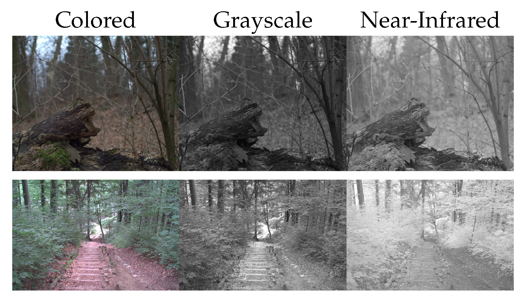
1.2.1. Colorizing NIR Images—Luminance and Chrominance
1.2.2. Colorizing NIR Images—Paired vs. Unpaired Image Translation
1.2.3. Colorizing NIR Images—GAN-Based Approaches vs. Diffusion Models
1.2.4. Colorizing NIR Images: Refined Contribution
- Replacing the low-pass filter as latent variable refinement technique;
- Differentiating into merging chrominance and merging intensity instead;
- Abstracting the intensity translation.
1.3. Related Work
1.3.1. GAN-Based Approaches
1.3.2. Diffusion Models
2. Materials and Methods
2.1. Background
2.2. Iterative Seeding
| Algorithm 1 Iterative Seeding |
|
2.2.1. Near-Infrared Intensities
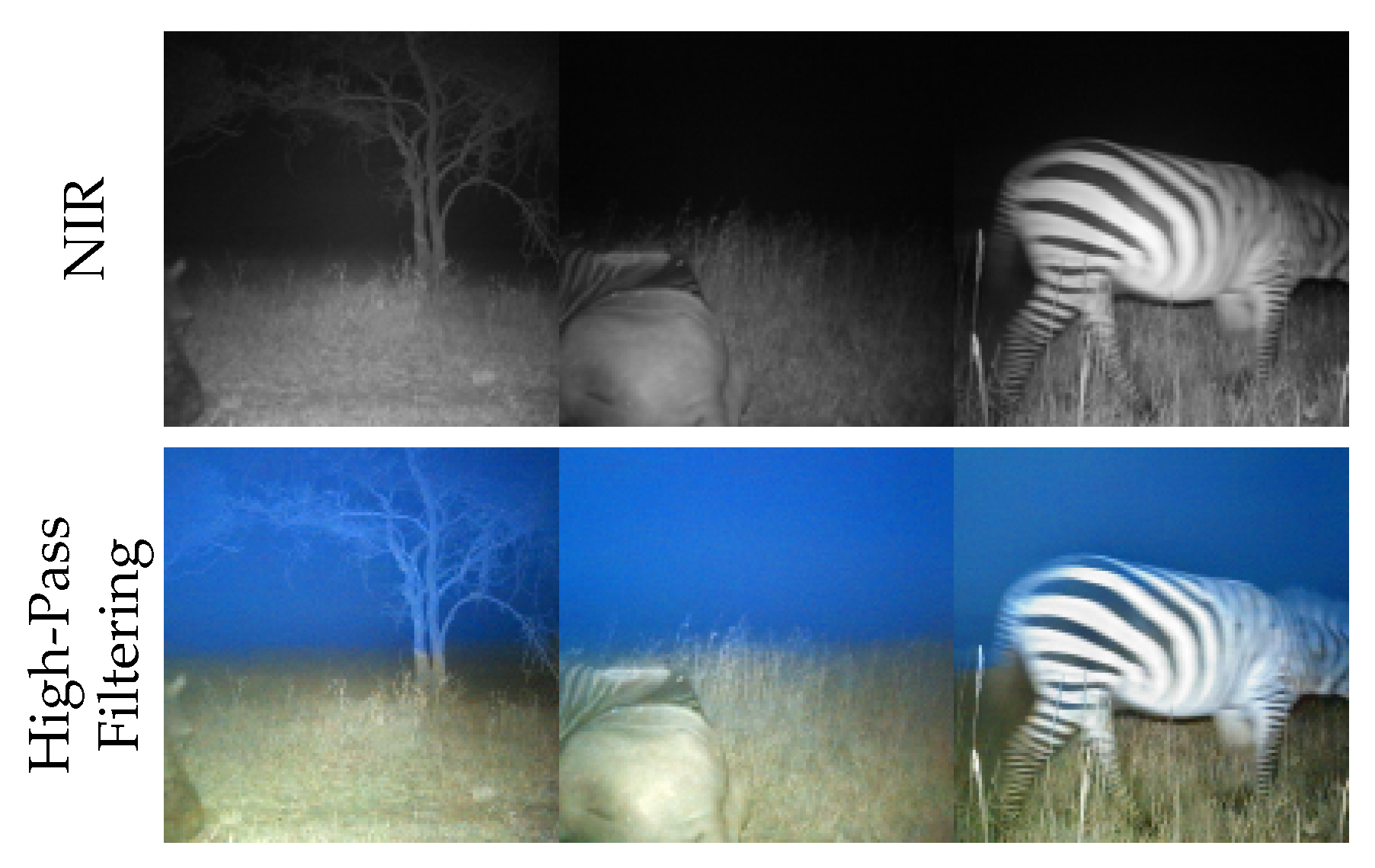
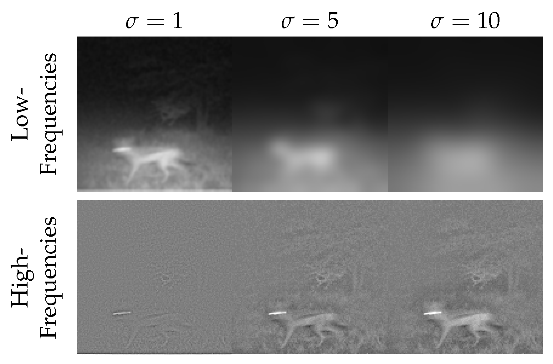
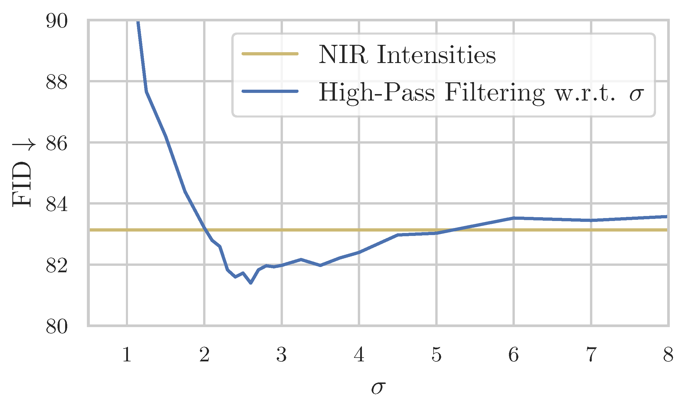
2.2.2. High-Pass Filtering
| Algorithm 2 Implementation using High-Pass Filtering |
|
3. Experimental Results
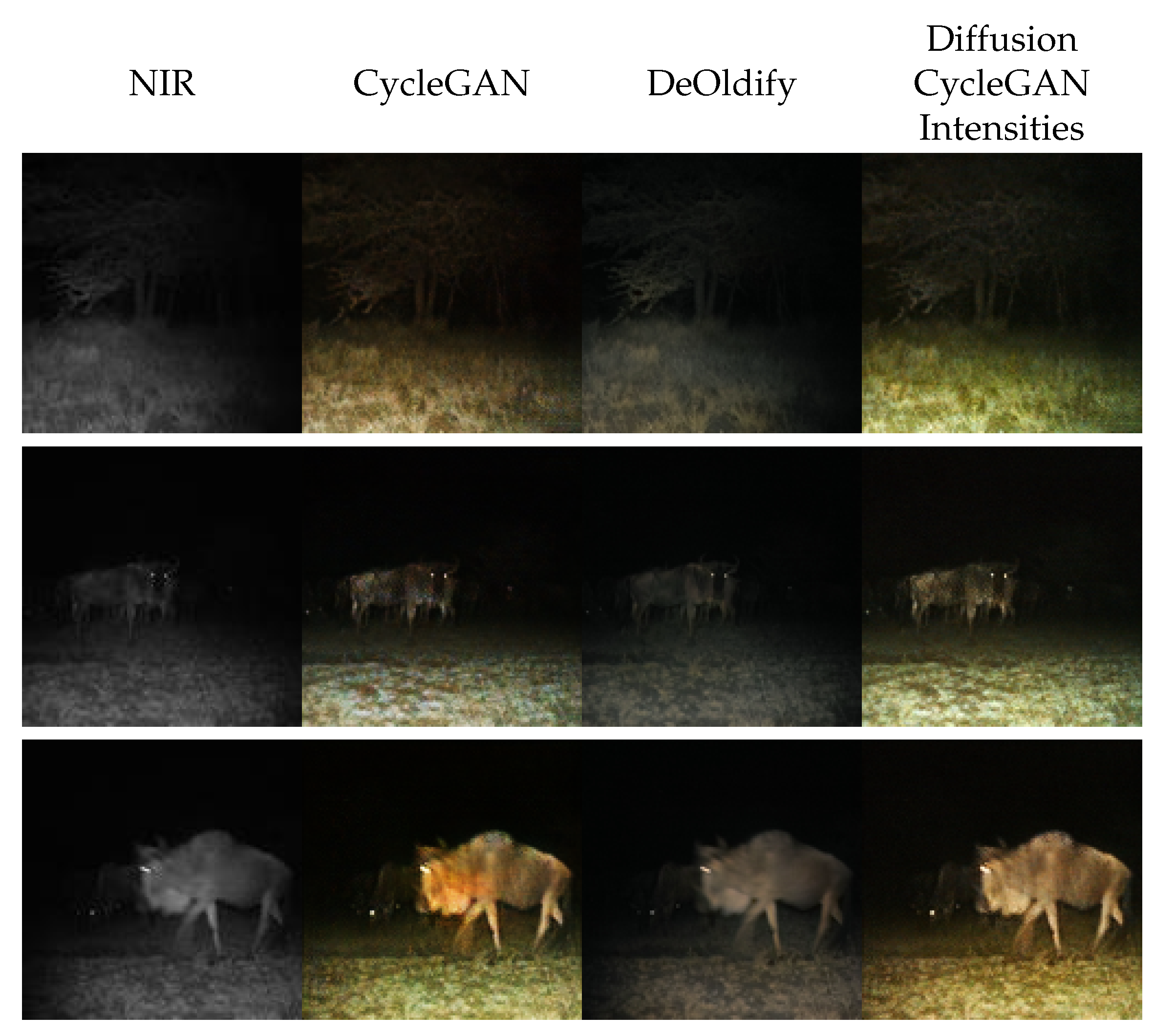
3.1. The Identity—Using Near-Infrared Intensities
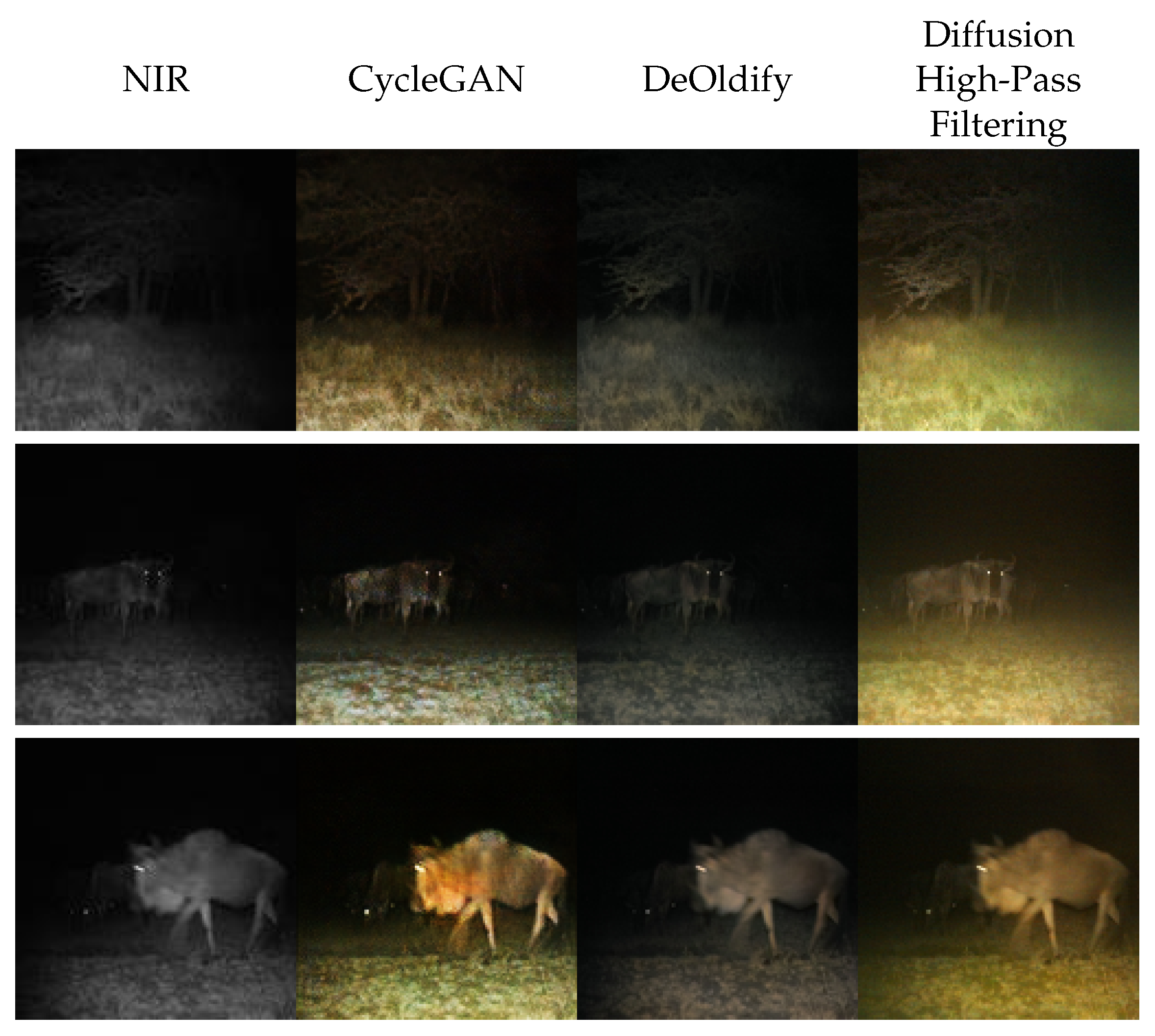
3.2. Fusing Near-Infrared and Visible Intensity through High-Pass Filtering
3.3. The Potential of Diffusion-Based Near-Infrared Colorization—CycleGAN as Intensity Translation Function
4. Discussion
4.1. Implementations of Intensity Translation
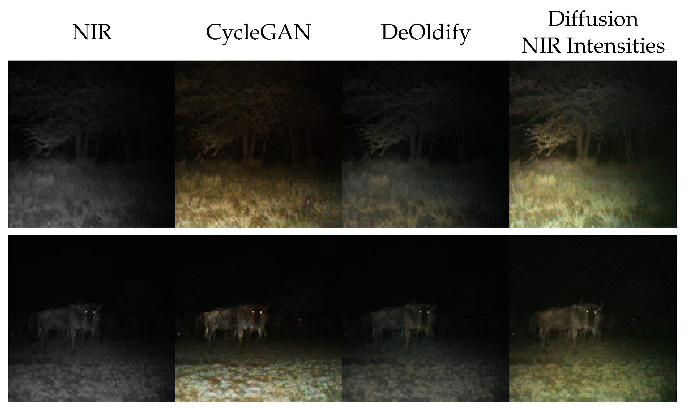
- We demonstrate directly using the NIR intensity, effectively representing an identity function. This simple implementation creates a basic colorization, but the diffusion network is too restricted by the NIR intensity, yielding suboptimal realism and FID scores. Even though this colorization is not specialized for near-infrared colorization, it performs more robustly than other grayscale colorization methods, as the comparison with DeOldify suggests.
- Because the framework can be considered iteratively fusing near-infrared and visible light, we draw inspiration from the VIS-NIR fusion research domain. A key observation made in this field is to use the high-frequency intensities of the near-infrared image and fuse them with the low-frequency intensities of the visible-light image. We apply this insight to our framework in a trivial implementation using a Gaussian filter. An improvement in comparison with just using the NIR images as intensities is observed quantitatively and qualitatively, resulting in an FID score close to our baseline CycleGAN. Additionally, with the ClipFID, a different FID variant not relying on the Inception model and the ImageNet dataset [42], we achieve a score of using this translation method compared to CycleGAN . However, because the ClipFID is not established as a comparison metric, this result has to be treated carefully. Even though this implementation is far from exhausting results from the VIS-NIR fusion domain, it achieves scores close to our baseline, suggesting a more sophisticated implementation can achieve even better results.
- Finally, we evaluate CycleGAN itself as an intensity translator. Using intensities generated by CycleGAN our framework outperforms CycleGAN quantitatively as well as qualitatively. This indicates the potential of our framework for sophisticated translation functions and diffusion-based NIR colorization in general. Considering this potential, we show that our framework reduces NIR colorization to visible near-infrared fusion, a simpler problem.
4.2. Colorizing NIR Images for Animal Detection
4.3. Colorizing NIR Images for Animal Detection Explainability
4.4. Novelty and Scientific Relevance
4.5. Limitations and Challenges
5. Conclusions
- Iterative Seeding on NIR intensities (ISNIR);
- Iterative Seeding using high-pass filtering (ISHP);
- Iterative Seeding using CycleGAN intensities (ISCG).
5.1. Future Work
Author Contributions
Funding
Institutional Review Board Statement
Informed Consent Statement
Data Availability Statement
Acknowledgments
Conflicts of Interest
Abbreviations
| NIR | near-infrared |
| RGB | red, green, blue (color channels) |
| VIS-NIR fusion | visible-near-infrared fusion |
| GAN | generative adversarial network |
| ILVR | iterative latent variable refinement |
| FID | Fréchet inception distance |
| CNN | convolutional neural network |
References
- Haucke, T.; Kühl, H.S.; Hoyer, J.; Steinhage, V. Overcoming the distance estimation bottleneck in estimating animal abundance with camera traps. Ecol. Inform. 2022, 68, 101536. [Google Scholar] [CrossRef]
- Palencia, P.; Fernández-López, J.; Vicente, J.; Acevedo, P. Innovations in movement and behavioural ecology from camera traps: Day range as model parameter. Methods Ecol. Evol. 2021, 12, 1201–1212. [Google Scholar] [CrossRef]
- Schindler, F.; Steinhage, V.; van Beeck Calkoen, S.T.S.; Heurich, M. Action Detection for Wildlife Monitoring with Camera Traps Based on Segmentation with Filtering of Tracklets (SWIFT) and Mask-Guided Action Recognition (MAROON). Appl. Sci. 2024, 14, 514. [Google Scholar] [CrossRef]
- Oliver, R.Y.; Iannarilli, F.; Ahumada, J.; Fegraus, E.; Flores, N.; Kays, R.; Birch, T.; Ranipeta, A.; Rogan, M.S.; Sica, Y.V.; et al. Camera trapping expands the view into global biodiversity and its change. Philos. Trans. R. Soc. B Biol. Sci. 2023, 378, 20220232. [Google Scholar] [CrossRef]
- Green, S.E.; Stephens, P.A.; Whittingham, M.J.; Hill, R.A. Camera trapping with photos and videos: Implications for ecology and citizen science. Remote Sens. Ecol. Conserv. 2023, 9, 268–283. [Google Scholar] [CrossRef]
- Edelman, A.J.; Edelman, J.L. An Inquiry-Based Approach to Engaging Undergraduate Students in On-Campus Conservation Research Using Camera Traps. Southeast. Nat. 2017, 16, 58–69. [Google Scholar] [CrossRef]
- Wägele, J.W.; Bodesheim, P.; Bourlat, S.J.; Denzler, J.; Diepenbroek, M.; Fonseca, V.G.; Frommolt, K.H.; Geiger, M.F.; Gemeinholzer, B.; Glöckner, F.O.; et al. Towards a multisensor station for automated biodiversity monitoring. Basic Appl. Ecol. 2022, 59, 105–138. [Google Scholar] [CrossRef]
- Swanson, A.; Kosmala, M.; Lintott, C.; Simpson, R.; Smith, A.; Packer, C. Data from: Snapshot Serengeti, high-frequency annotated camera trap images of 40 mammalian species in an African savanna. Sci. Data 2015, 2, 150026. [Google Scholar] [CrossRef]
- ISO 20473:2007; Optics and Photonics—Spectral Bands. International Organization for Standardization: Geneva, Switzerland, 2007.
- Toet, A.; Hogervorst, M.A. Progress in color night vision. Opt. Eng. 2012, 51, 010901. [Google Scholar] [CrossRef]
- Adam, M.; Tomášek, P.; Lehejček, J.; Trojan, J.; Jůnek, T. The Role of Citizen Science and Deep Learning in Camera Trapping. Sustainability 2021, 13, 287. [Google Scholar] [CrossRef]
- Simões, F.; Bouveyron, C.; Precioso, F. DeepWILD: Wildlife Identification, Localisation and estimation on camera trap videos using Deep learning. Ecol. Inform. 2023, 75, 102095. [Google Scholar] [CrossRef]
- Gao, R.; Zheng, S.; He, J.; Shen, L. CycleGAN-Based Image Translation for Near-Infrared Camera-Trap Image Recognition. In Proceedings of the Pattern Recognition and Artificial Intelligence: International Conference, ICPRAI 2020, Zhongshan, China, 19–23 October 2020; Springer International Publishing: Cham, Switzerland, 2020; pp. 453–464. [Google Scholar]
- Mehri, A.; Sappa, A.D. Colorizing near infrared images through a cyclic adversarial approach of unpaired samples. In Proceedings of the IEEE/CVF Conference on Computer Vision and Pattern Recognition Workshops, Long Beach, CA, USA, 16–17 June 2019. [Google Scholar]
- Metz, L.; Poole, B.; Pfau, D.; Sohl-Dickstein, J. Unrolled generative adversarial networks. arXiv 2016, arXiv:1611.02163. [Google Scholar]
- Ho, J.; Jain, A.; Abbeel, P. Denoising diffusion probabilistic models. Adv. Neural Inf. Process. Syst. 2020, 33, 6840–6851. [Google Scholar]
- Dhariwal, P.; Nichol, A. Diffusion models beat gans on image synthesis. Adv. Neural Inf. Process. Syst. 2021, 34, 8780–8794. [Google Scholar]
- Song, Y.; Sohl-Dickstein, J.; Kingma, D.P.; Kumar, A.; Ermon, S.; Poole, B. Score-based generative modeling through stochastic differential equations. arXiv 2020, arXiv:2011.13456. [Google Scholar]
- Choi, J.; Kim, S.; Jeong, Y.; Gwon, Y.; Yoon, S. Ilvr: Conditioning method for denoising diffusion probabilistic models. arXiv 2021, arXiv:2108.02938. [Google Scholar]
- Sharma, A.M.; Dogra, A.; Goyal, B.; Vig, R.; Agrawal, S. From pyramids to state-of-the-art: A study and comprehensive comparison of visible–infrared image fusion techniques. IET Image Process. 2020, 14, 1671–1689. [Google Scholar] [CrossRef]
- Limmer, M.; Lensch, H.P. Infrared colorization using deep convolutional neural networks. In Proceedings of the 2016 15th IEEE International Conference on Machine Learning and Applications (ICMLA), Anaheim, CA, USA, 18–20 December 2016; pp. 61–68. [Google Scholar]
- Dong, Z.; Kamata, S.i.; Breckon, T.P. Infrared image colorization using a s-shape network. In Proceedings of the 2018 25th IEEE International Conference on Image Processing (ICIP), Athens, Greece, 7–10 October 2018; pp. 2242–2246. [Google Scholar]
- Zhu, J.Y.; Park, T.; Isola, P.; Efros, A.A. Unpaired image-to-image translation using cycle-consistent adversarial networks. In Proceedings of the IEEE International Conference on Computer Vision, Venice, Italy, 22–29 October 2017; pp. 2223–2232. [Google Scholar]
- He, K.; Zhang, X.; Ren, S.; Sun, J. Deep residual learning for image recognition. In Proceedings of the IEEE Conference on Computer Vision and Pattern Recognition, Las Vegas, NV, USA, 27–30 June 2016; pp. 770–778. [Google Scholar]
- Antic, J. Deoldify. Available online: https://github.com/jantic/DeOldify (accessed on 24 January 2024).
- Sohl-Dickstein, J.; Weiss, E.; Maheswaranathan, N.; Ganguli, S. Deep unsupervised learning using nonequilibrium thermodynamics. In Proceedings of the International Conference on Machine Learning, PMLR, Lille, France, 7–9 July 2015; pp. 2256–2265. [Google Scholar]
- Song, Y.; Ermon, S. Generative modeling by estimating gradients of the data distribution. In Proceedings of the Advances in Neural Information Processing Systems, Vancouver, BC, Canada, 8–14 December 2019; Volume 32. [Google Scholar]
- Welling, M.; Teh, Y.W. Bayesian learning via stochastic gradient Langevin dynamics. In Proceedings of the 28th International Conference on Machine Learning (ICML-11), Bellevue, WA, USA, 28 June–2 July 2011; pp. 681–688. [Google Scholar]
- Saharia, C.; Chan, W.; Chang, H.; Lee, C.; Ho, J.; Salimans, T.; Fleet, D.; Norouzi, M. Palette: Image-to-image diffusion models. In Proceedings of the ACM SIGGRAPH 2022 Conference Proceedings, Vancouver, BC, Canada, 7–11 August 2022; pp. 1–10. [Google Scholar]
- Zhao, M.; Bao, F.; Li, C.; Zhu, J. Egsde: Unpaired image-to-image translation via energy-guided stochastic differential equations. Adv. Neural Inf. Process. Syst. 2022, 35, 3609–3623. [Google Scholar]
- Zhu, Y.; Sun, X.; Zhang, H.; Wang, J.; Fu, X. Near-infrared and visible fusion for image enhancement based on multi-scale decomposition with rolling WLSF. Infrared Phys. Technol. 2023, 128, 104434. [Google Scholar] [CrossRef]
- Bulanon, D.; Burks, T.; Alchanatis, V. Image fusion of visible and thermal images for fruit detection. Biosyst. Eng. 2009, 103, 12–22. [Google Scholar] [CrossRef]
- Ronneberger, O.; Fischer, P.; Brox, T. U-net: Convolutional networks for biomedical image segmentation. In Medical Image Computing and Computer-Assisted Intervention; Springer: Berlin/Heidelberg, Germany, 2015; pp. 234–241. [Google Scholar]
- Forsyth, D.A.; Ponce, J. Computer Vision: A Modern Approach; Prentice Hall: Upper Saddle River, NJ, USA, 2002. [Google Scholar]
- Wang, Z.; Bovik, A.C.; Sheikh, H.R.; Simoncelli, E.P. Image quality assessment: From error visibility to structural similarity. IEEE Trans. Image Process. 2004, 13, 600–612. [Google Scholar] [CrossRef] [PubMed]
- Heusel, M.; Ramsauer, H.; Unterthiner, T.; Nessler, B.; Hochreiter, S. Gans trained by a two time-scale update rule converge to a local nash equilibrium. In Proceedings of the Advances in Neural Information Processing Systems, Long Beach, CA, USA, 4–9 December 2017; Volume 30. [Google Scholar]
- Parmar, G.; Zhang, R.; Zhu, J.Y. On aliased resizing and surprising subtleties in gan evaluation. In Proceedings of the IEEE/CVF Conference on Computer Vision and Pattern Recognition, New Orleans, LA, USA, 18–24 June 2022; pp. 11410–11420. [Google Scholar]
- Mittal, A.; Soundararajan, R.; Bovik, A.C. Making a “completely blind” image quality analyzer. IEEE Signal Process. Lett. 2012, 20, 209–212. [Google Scholar] [CrossRef]
- Ma, C.; Yang, C.Y.; Yang, X.; Yang, M.H. Learning a no-reference quality metric for single-image super-resolution. Comput. Vis. Image Underst. 2017, 158, 1–16. [Google Scholar] [CrossRef]
- Brown, M.; Süsstrunk, S. Multi-spectral SIFT for scene category recognition. In Proceedings of the CVPR 2011, Colorado Springs, CO, USA, 20–25 June 2011; pp. 177–184. [Google Scholar]
- Sharma, V.; Hardeberg, J.Y.; George, S. RGB–NIR image enhancement by fusing bilateral and weighted least squares filters. In Proceedings of the Color and Imaging Conference, Society for Imaging Science and Technology, Scottsdale, AZ, USA, 13–17 November 2017; Volume 2017, pp. 330–338. [Google Scholar]
- Kynkäänniemi, T.; Karras, T.; Aittala, M.; Aila, T.; Lehtinen, J. The Role of ImageNet Classes in Fréchet Inception Distance. arXiv 2022, arXiv:2203.06026. [Google Scholar]
- Deng, J.; Dong, W.; Socher, R.; Li, L.J.; Li, K.; Fei-Fei, L. Imagenet: A large-scale hierarchical image database. In Proceedings of the 2009 IEEE Conference on Computer Vision and Pattern Recognition, Miami, FL, USA, 20–25 June 2009; pp. 248–255. [Google Scholar]
- Loyola-González, O. Black-Box vs. White-Box: Understanding Their Advantages and Weaknesses From a Practical Point of View. IEEE Access 2019, 7, 154096–154113. [Google Scholar] [CrossRef]
- Rombach, R.; Blattmann, A.; Lorenz, D.; Esser, P.; Ommer, B. High-resolution image synthesis with latent diffusion models. In Proceedings of the IEEE/CVF Conference on Computer Vision and Pattern Recognition, New Orleans, LA, USA, 18–24 June 2022; pp. 10684–10695. [Google Scholar]
- Song, J.; Meng, C.; Ermon, S. Denoising diffusion implicit models. arXiv 2020, arXiv:2010.02502. [Google Scholar]


| Model | FID ↓ |
|---|---|
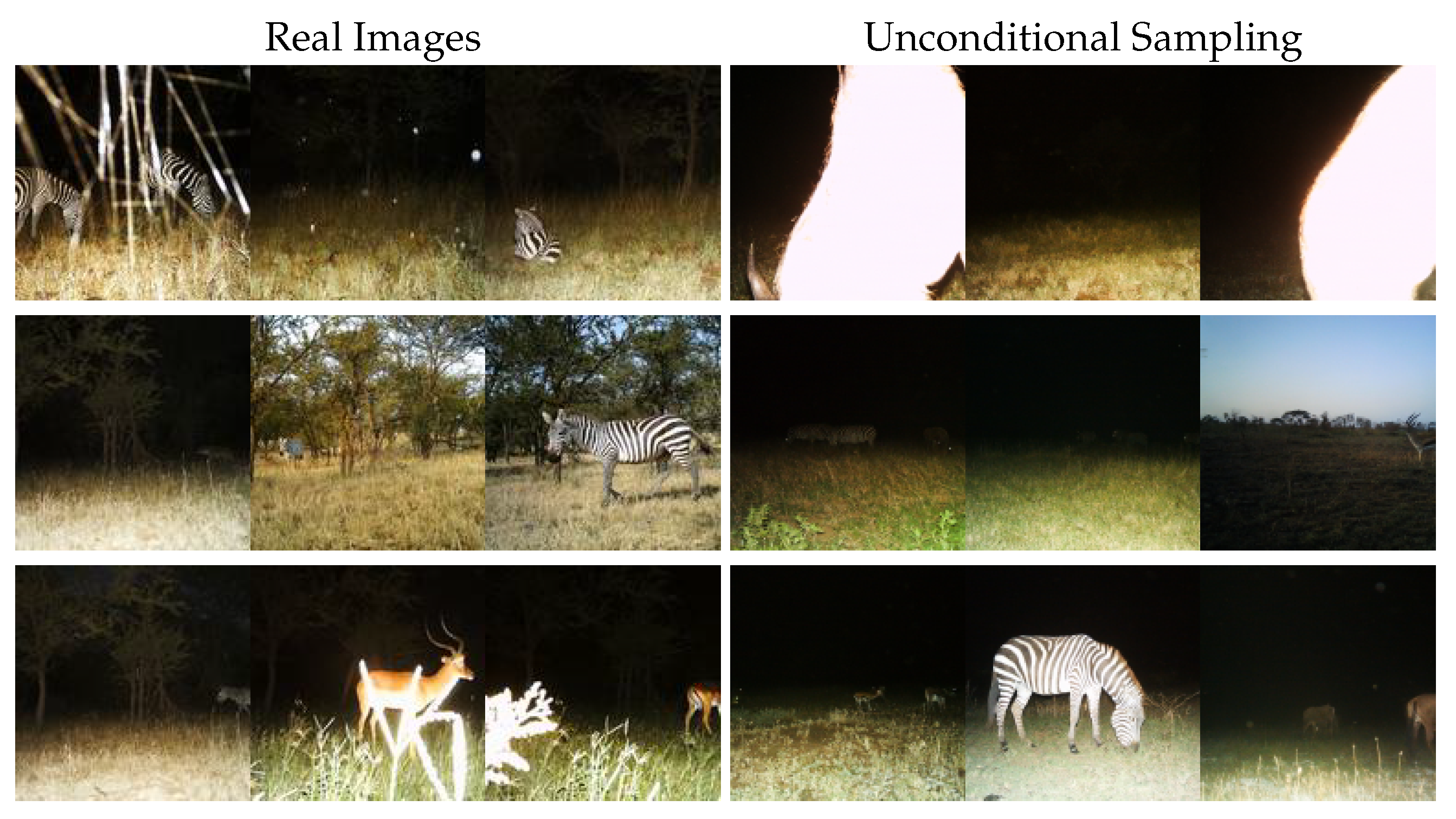
| Unconditional Diffusion Model [17] | 55.01 |
| Model | FID ↓ | NIQE ↓ | NRQM ↑ |
|---|---|---|---|
| CycleGAN [14] | |||
| DeOldify [25] | |||
| Iterative Seeding Using NIR Intensities |
| Model | FID ↓ | NIQE ↓ | NRQM ↑ |
|---|---|---|---|
| CycleGAN [14] | |||
| DeOldify [25] | |||
| Iterative Seeding High-Pass Filtering |
| Model | FID ↓ | NIQE ↓ | NRQM ↑ |
|---|---|---|---|
| CycleGAN [14] | |||
| DeOldify [25] | |||
| Iterative Seeding CycleGAN Intensities |
| Non-Frozen | Frozen | ||||
|---|---|---|---|---|---|
| Model | FID ↓ | Accuracy↑ | Accuracy ↑ | ||
| NIR | - | ||||
| CycleGAN [14] | |||||
| NIR Intensities | |||||
| High-Pass Filtering | |||||
| CycleGAN Intensities | |||||
Disclaimer/Publisher’s Note: The statements, opinions and data contained in all publications are solely those of the individual author(s) and contributor(s) and not of MDPI and/or the editor(s). MDPI and/or the editor(s) disclaim responsibility for any injury to people or property resulting from any ideas, methods, instructions or products referred to in the content. |
© 2024 by the authors. Licensee MDPI, Basel, Switzerland. This article is an open access article distributed under the terms and conditions of the Creative Commons Attribution (CC BY) license (https://creativecommons.org/licenses/by/4.0/).
Share and Cite
Borstelmann, A.; Haucke, T.; Steinhage, V. The Potential of Diffusion-Based Near-Infrared Image Colorization. Sensors 2024, 24, 1565. https://doi.org/10.3390/s24051565
Borstelmann A, Haucke T, Steinhage V. The Potential of Diffusion-Based Near-Infrared Image Colorization. Sensors. 2024; 24(5):1565. https://doi.org/10.3390/s24051565
Chicago/Turabian StyleBorstelmann, Ayk, Timm Haucke, and Volker Steinhage. 2024. "The Potential of Diffusion-Based Near-Infrared Image Colorization" Sensors 24, no. 5: 1565. https://doi.org/10.3390/s24051565
APA StyleBorstelmann, A., Haucke, T., & Steinhage, V. (2024). The Potential of Diffusion-Based Near-Infrared Image Colorization. Sensors, 24(5), 1565. https://doi.org/10.3390/s24051565