
Multivariable Air-Quality Prediction and Modelling via Hybrid Machine Learning: A Case Study for Craiova, Romania


Abstract
1. Introduction

| Ref. | A Brief Description | Objective Function | Data Location and Source | Predictors | Time-Series | Strengths | Limitation |
|---|---|---|---|---|---|---|---|
| [17] | An automated air quality forecasting system is developed for daily forecasts based on five various ML models: MLR, MLP, RF, GBDT, and SVR, combined with an FS technique. | PM2.5, PM10, SO2, NO2, O3, CO | Seven cities in China: Beijing, Shanghai, Guangzhou, Chengdu, Xi’an, Wuhan, and Changchun. (http://www.cnemc.cn) (accessed on 15 January 2022). | Daily pressure, 2 m temperature, relative humidity, precipitation, visibility, and total cloud cover. (http://data.cma.cn) (accessed on 15 January 2022). | Daily average | Development of an automated air quality forecasting system based on five various ML models. | Feature importance scores were calculated by the RF model, in which the predictor variables were checked individually. |
| [14] | Hybrid model based on a deterministic prediction module (RF-ELM) combined with an interval prediction module. | PM2.5 | Three major cities in China are Guang Zhou, Shenzhen, and Zhuhai. | ---- | Daily average | The use of an interval prediction module. | These are very complex models. |
| [15] | RF model combined with a meteorological normalization method. | PM2.5 | Hubei Province, China. https://quotsoft.net/air/ (accessed on 15 January 2022). | Included 2 m temperature, 2 m dewpoint temperature, 10 m u-component of wind, 10 m v-component of wind, surface pressure, total precipitation, boundary layer height, and downward surface solar radiation. | Hourly | The use of a meteorological normalization method. | Only a quantification of air pollution was performed. No forecasting and/or modelling was made. |
| [16] | Hybrid air quality forecasting system based on relief-F algorithm combined with a MOCBO and a modified fuzzy neural network. | AQI | Shanghai, Hangzhou, and Nanjing are three regions with severe air pollution in China. | PM2.5, PM10, SO2, CO, NO2, and O3 concentrations, average temperature (°C), cumulative precipitation (CP, mm), average wind speed (AWS, m/s), and average relative humidity. | Daily average | A comparison with other ML models and FS methods. | One combination of inputs was found for AQI forecasting. |
| [13] | MDA, Bagged CART, and RF combined with SA. | PM10 | A total of 75 stations over Barcelona, Spain. | Minimum temperature, maximum temperature, normalized difference vegetation index, precipitation, wind speed, wind direction, elevation, road density, topographic wetness index, land use, terrain roughness index, distance from water body, land use, and lithology. | Annually average | The use of many FS-ML models and comparison with others. | One combination of inputs was found for PM10 forecasting. |
| [18] | An ANN model was used to forecast daily pollutant concentrations. Real-time correlation (RTC) was applied to improve the quality of the forecasts. | PM10, PM2.5, NO2, and O3 | A total of 32 continuous air-quality-monitoring stations in Delhi, India. | CAVG_DAY0 CAVG_DAYM1 BLH_DAYN T2M_DAYN RH_DAYN IS975_DAYN IS950_DAYN IS925_DAYN U10_DAYNM1_DAYN V10_DAYNM1_DAYN TP_DAYN FIRE_DAYNM3_DAYNM1. | Daily average | Application of Real-Time Correction (RTC) technique. | ANN is a stochastic method, which means that one cannot obtian the same results for the same dataset. No FS was applied. |
| [19] | A hybrid early-warning artificial intelligence framework (ICEEMDAN-OS-ELM) was proposed. | PM2.5, PM10, and lower atmospheric visibility | Gladstone, Brisbane, Mackay Region, Newcastle, and Sydney, Australia. | --- | Hourly | The results are benchmarked with many ML models. | The main common weakness is that one should have data (measures) for obtaining data (forecasts). |
| [20] | Forecasting AQI using a long short-term memory (LSTM) neural network model combined with a variational mode decomposition (VMD) and a sample entropy. | AQI | Beijing and Baoding, China. https://www.aqistudy.cn/historydata/ (accessed on 15 January 2022). | --- | Daily average | A comparison with other models was performed. | No FS was applied. |
| [21] | Air pollutant concentration forecasting was performed by combining an EWT decomposition algorithm with MAEGA and NARX neural networks. | PM2.5, SO2, NO2, CO | Beijing in China. | --- | --- | A comparison was made with the VMD-MAEGA-NARX, EWT-MAEGA-SVM, MAEGA-NARX, EWT-NARX, and EWT-ARIMA-NARX models. | No inputs and no FS were applied. |
| [22] | A dynamic multiple equation (DME) model (a linear model). | PM2.5 | Santiago, Chile. | Temperature, wind speed, relative humidity, wind direction, and CO. | Hourly and daily average | A comparison with SARI-MAX and ANN models. | Complex model structure. |
- i.
- Implementing an Autonomous Anomaly Detection method during data preprocessing to identify and exclude anomalous data points.
- ii.
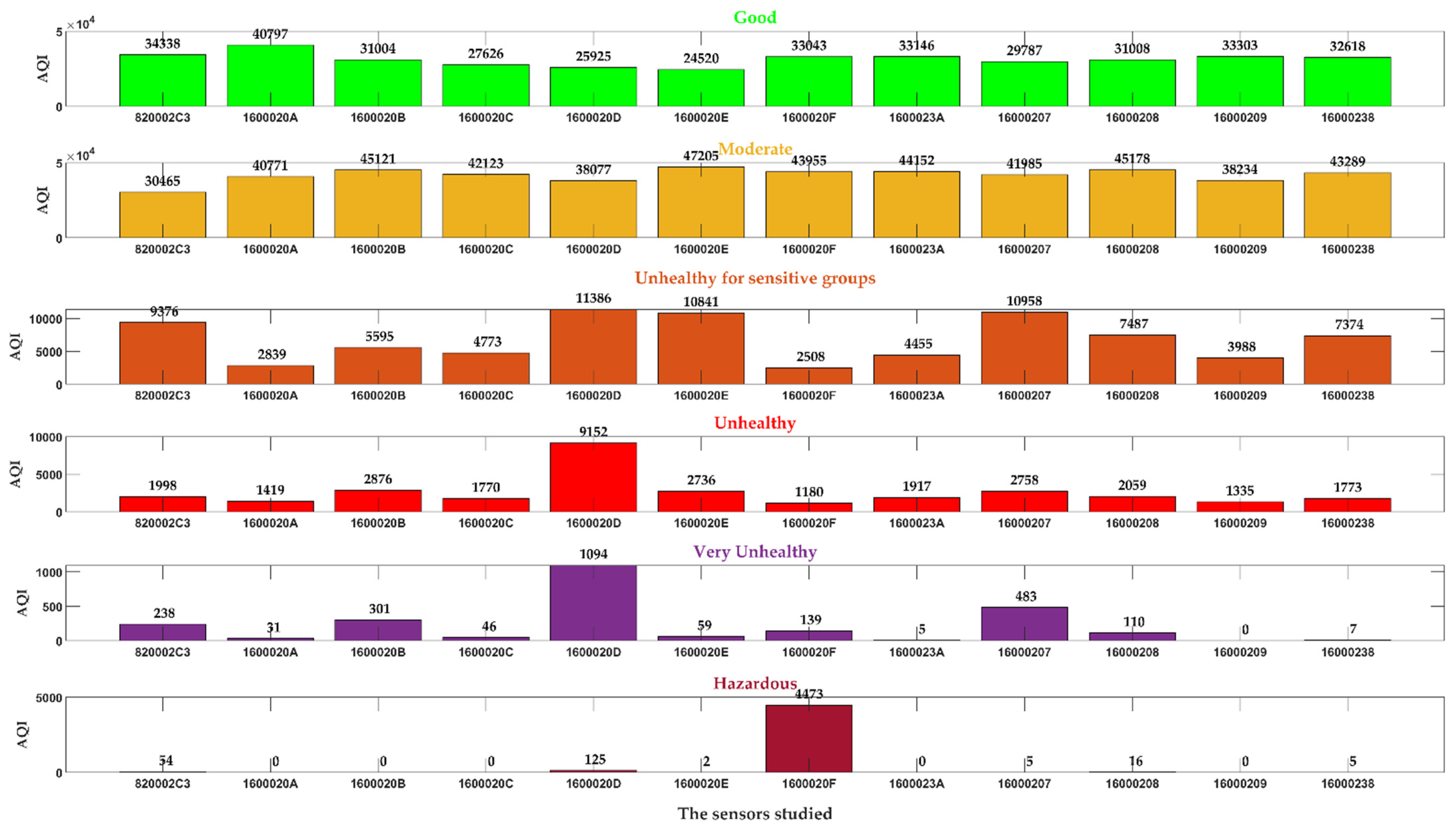
- Identifying spatial and temporal hazards detected by the study’s sensors/stations.
- iii.
- Clustering and decomposing data based on the significance of AQI in terms of health implications.
- iv.
- Analyzing partial dependence and estimating the importance of each predictor variable considered.
- v.
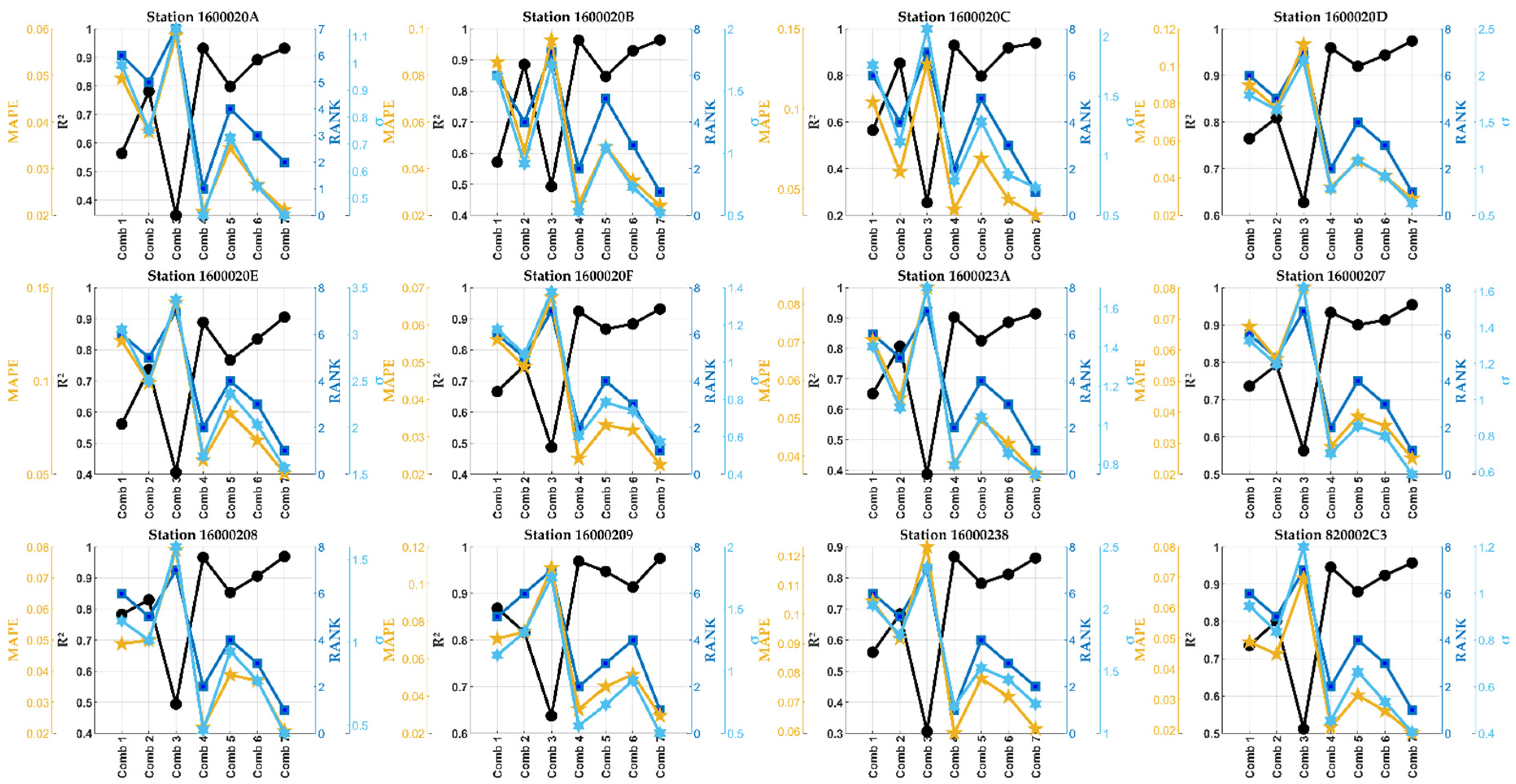
- Determining the optimal combinations of predictor variables for predicting AQI and other related pollutant concentrations through a comprehensive FS approach.
- vi.
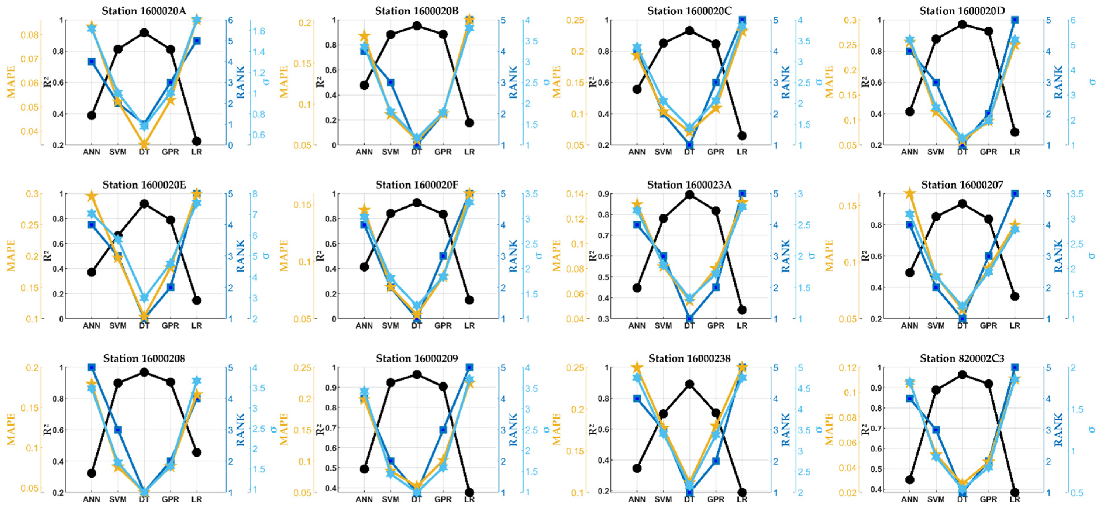
- Evaluating the performance of five hybrid FS-ML models for predicting a one-minute series of PM10, PM2.5, and PM1 and then AQI.
- vii.
- Developing new physical models for estimating PM10, PM2.5, PM1, and AQI.
- viii.
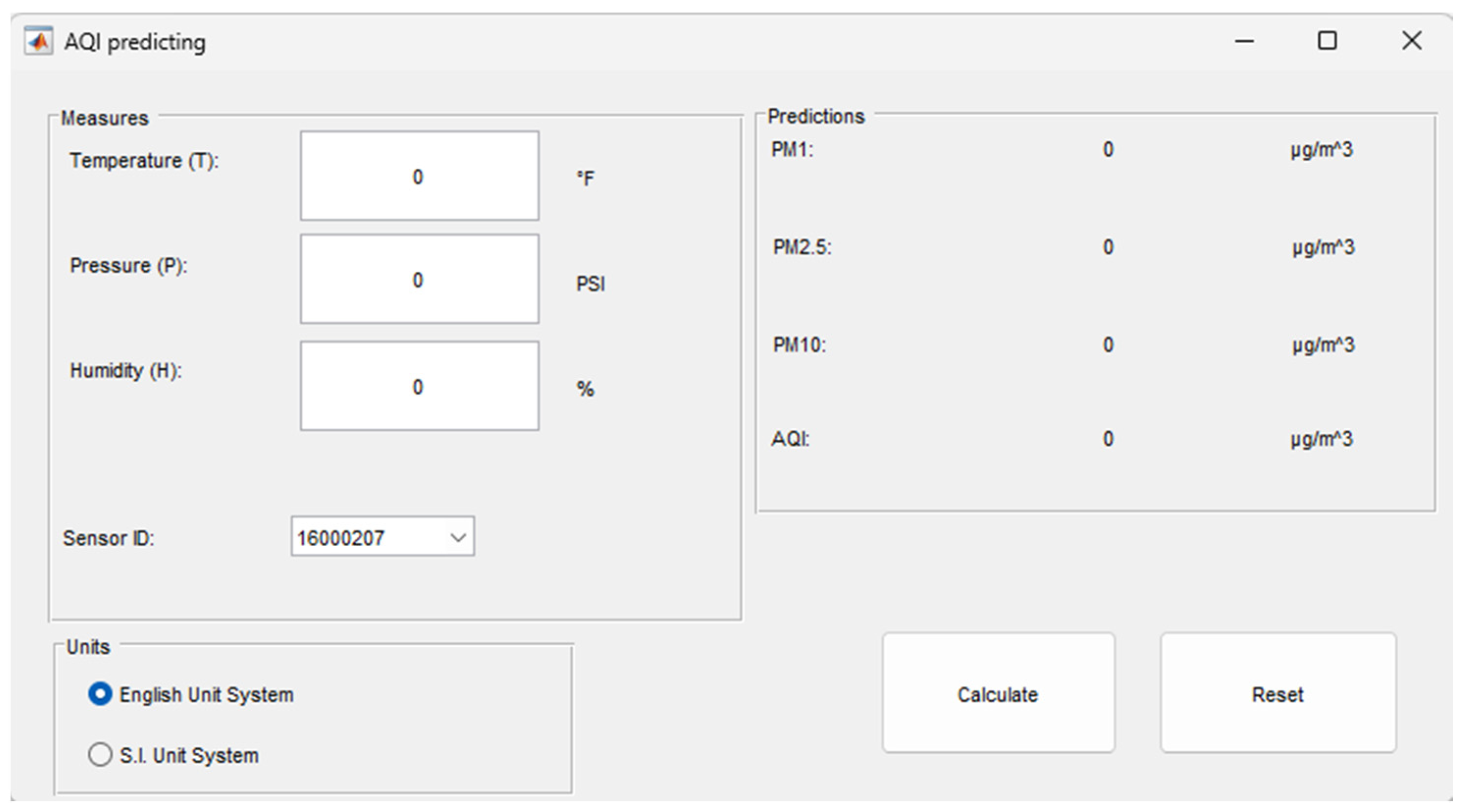
- Creating a new interface module to provide PM10, PM2.5, PM1, and AQI predictions based on the provided predictor variables.
- i.
- Analyzing pollution episodes in Craiova in line with World Health Organization (WHO) recommendations.
- ii.
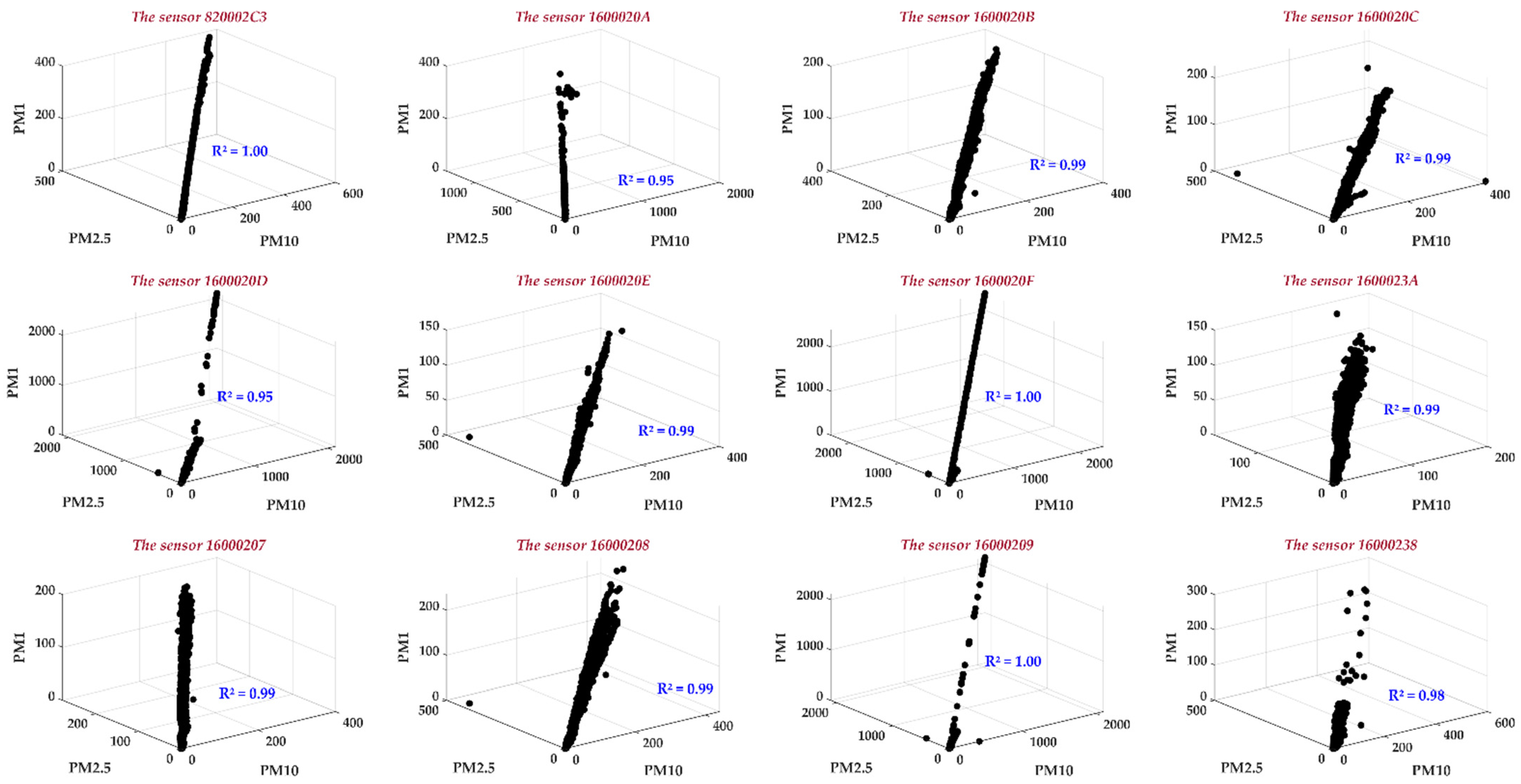
- Evaluating the correlations between meteorological parameters, AQI, and PM concentrations and interrelations among different PM fractions, such as PM1, PM2.5, and PM10.
- iii.
- Investigating the influences of noise and carbon dioxide (CO2) on PM concentrations.
2. Data and Statistical Analysis
2.1. Local Weather Information
2.2. Correlation between the PM1, PM2.5, and PM10 Concentrations
2.3. Evaluation Criteria and Statistical Indices
3. Hybrid FS-ML Models
3.1. Machine Learning Models
- i.
- Artificial Neural Network
- ii.
- Support Vector Machine
- iii.
- Decision Tree
- iv.
- Gaussian Process Regression
- v.
- Linear Regression
3.2. Feature Selection: Integral Feature Selection Method
3.3. Modelling: Least Square Regression
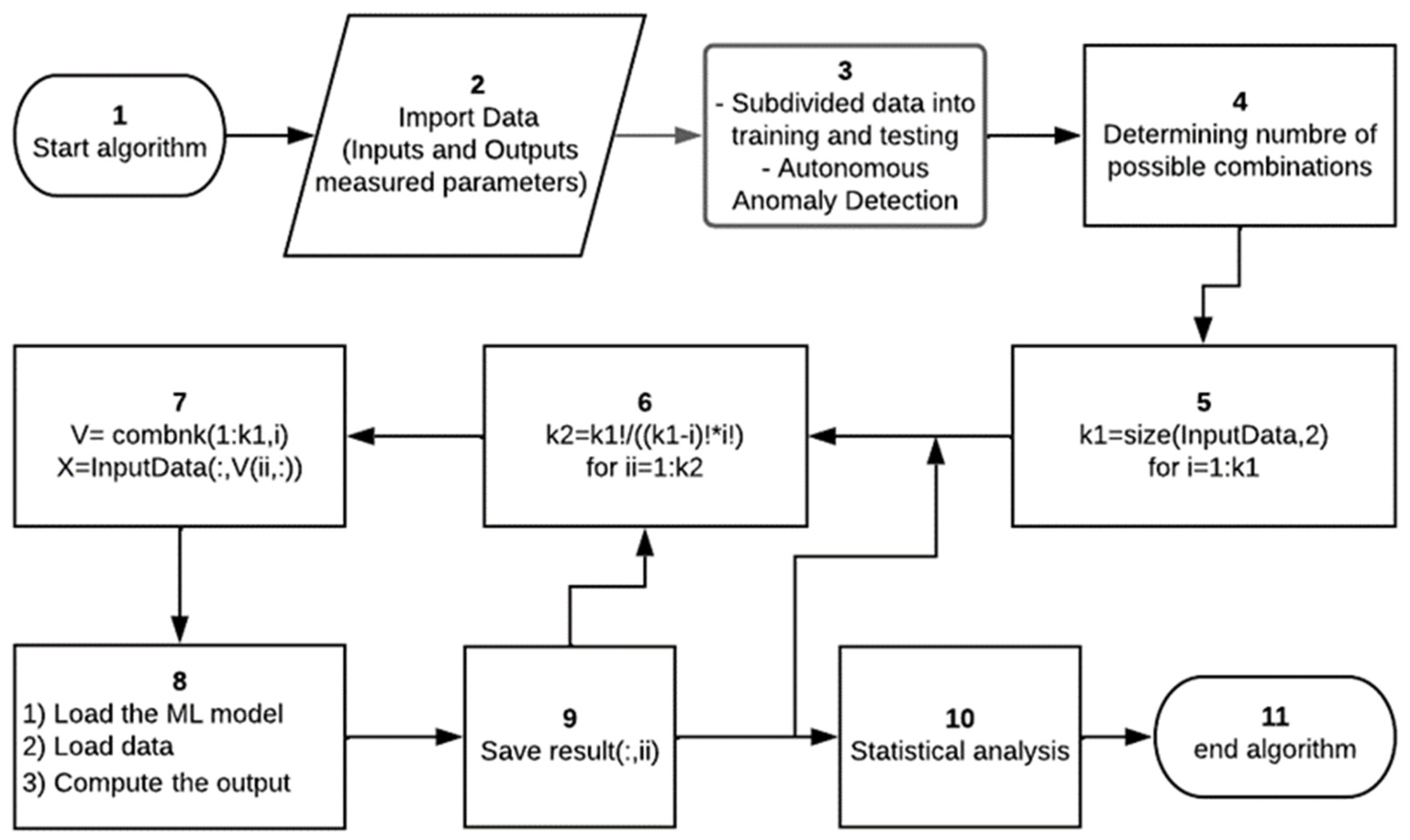
4. Methodology
- Start the algorithm.
- Import the inputs and outputs data.
- First, the data are pre-processed by applying normalization and Autonomous Anomaly Detection, are loaded to each studied ML model, and then are subdivided into training (80% of data) and testing (the remaining data).
- Compute the total number of combinations based on the data size loaded using Equation (11).
- Start a first loop based on the size of the provided data, K1.
- Compute the number of combinations for each ith considered size and then start a second loop for each value of K2.
- Use the combnk(V, K) function for producing a matrix with K columns.
- Load the ML model, load the data, and compute the considered output parameter.
- Save the computed values and go to the next iteration.
- After obtaining the predicted values by all considered combinations, the result is imported by a second algorithm in which the statistical analysis is performed.
- The best combinations of inputs are found and then the algorithm is ended.
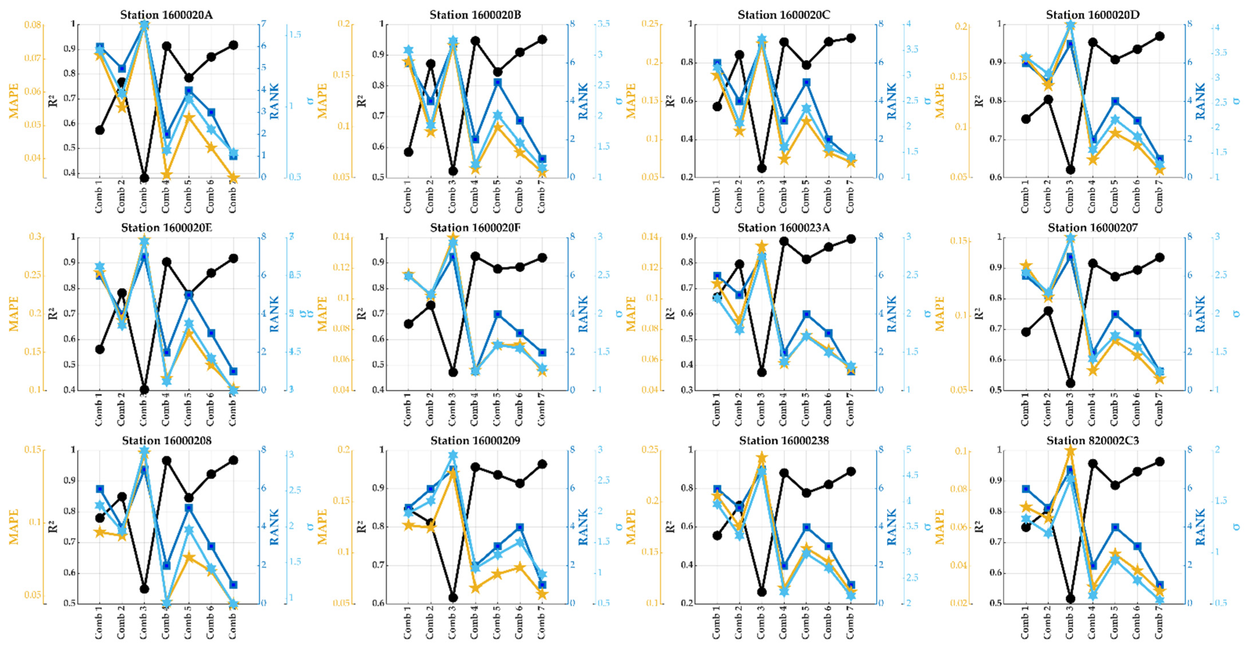
5. Results and Discussion
- -
- Comb1: Temperature
- -
- Comb2: Pressure
- -
- Comb3: Humidity
- -
- Comb4: Temperature and Pressure
- -
- Comb5: Temperature and Humidity
- -
- Comb6: Pressure and Humidity
- -
- Comb7: Temperature, Pressure, and Humidity
5.1. The Hybrid FS-DT Model Applied for Predicting PM1 Concentrations
5.2. Hybrid FS-DT Model Applied for Predicting PM2.5 Concentrations
5.3. Hybrid FS-DT Model Applied for Predicting PM10 Concentrations
5.4. Influence of VOC, Noise, and CO2 on PM Concentrations
5.5. Modelling of PMs and AQI
6. Conclusions
Author Contributions
Funding
Institutional Review Board Statement
Informed Consent Statement
Data Availability Statement
Conflicts of Interest
Appendix A
| Station | PM1 (μg/m3) | PM2.5 (μg/m3) | PM10 (μg/m3) | |||||||||
|---|---|---|---|---|---|---|---|---|---|---|---|---|
| a1 | a2 | a3 | a0 | a1 | a2 | a3 | a0 | a1 | a2 | a3 | a0 | |
| 820002C3 | 0 | 2.59 × 10⁻³ | −0.11 | −12.54 | 0 | 3.43 × 10⁻³ | −0.13 | −17.13 | 0 | 3.85 × 10⁻³ | −0.16 | −18.09 |
| 1600020A | 0.14 | 6.65 × 10⁻⁶ | 0 | 1.48 | 0.26 | −1.7 × 10⁻⁵ | 0.03 | 0.72 | 0.27 | 8.14 × 10⁻⁶ | 0 | 0.87 |
| 1600020B | 0 | −3.01 × 10⁻⁵ | 0.06 | 4.98 | 0 | −1.02 × 10⁻³ | 0.19 | 6.07 | 0 | −1.42 × 10⁻³ | 0.27 | 6.13 |
| 1600020C | 0 | 1.06 × 10⁻⁵ | −0.05 | 9.64 | 0 | 3.03 × 10⁻⁵ | −0.10 | 13.41 | 0 | 3.66 × 10⁻⁵ | −0.12 | 14.50 |
| 1600020D | 0 | 5.02 × 10⁻⁶ | −0.03 | 9.63 | 1.07 × 10⁻² | 1.2 × 10⁻⁵ | −0.06 | 13.69 | 0 | 2.05 × 10⁻⁵ | −0.09 | 16.02 |
| 1600020E | 1.69 | −7.59 × 10⁻³ | 0.93 | −0.70 | 2.84 | −1.26 × 10⁻² | 1.57 | −4.61 | 3.27 | −1.39 × 10⁻² | 1.67 | −2.58 |
| 1600020F | 0.22 | 2.25 × 10⁻⁵ | 0 | −1.46 | 1.83 | −1.17 × 10⁻² | 1.43 | 0.13 | 2.08 | −1.36 × 10⁻² | 1.66 | 0.23 |
| 1600023A | 0.48 | 1.56 × 10⁻⁶ | 0 | −0.24 | 1.9 | −6.21 × 10⁻³ | 0.75 | 0.33 | 0 | 5.53 × 10⁻³ | −0.20 | −33.02 |
| 16000207 | 0 | −1.37 × 10⁻³ | −0.12 | 33.86 | 0 | −9.95 × 10⁻⁵ | −0.25 | 36.49 | 0 | −3.10 × 10⁻⁵ | −0.24 | 30.10 |
| 16000208 | 0 | −5.64 × 10⁻⁵ | 0.19 | −1.26 | 0 | −1.66 × 10⁻³ | 0.39 | −1.65 | 0 | −2.13 × 10⁻³ | 0.48 | −1.87 |
| 16000209 | 0 | 3.21 × 10⁻³ | −0.19 | −14.23 | 0.61 | 1.83 × 10⁻³ | −0.19 | −6.74 | 0 | 5.81 × 10⁻³ | −0.34 | −27.24 |
| 16000238 | 1.41 | −4.75 × 10⁻³ | 0.56 | 1.45 | 0.91 | −5.60 × 10⁻⁵ | 0.12 | −1.59 | 2.80 | −1.03 × 10⁻² | 1.27 | 1.51 |
References
- Global Air Quality Guidelines: Particulate Matter (PM2.5 and PM10), Ozone, Nitrogen Dioxide, Sulfur Dioxide, and Carbon Monoxide. 2021. Available online: https://www.who.int/publications/i/item/9789240034228 (accessed on 19 January 2022).
- WHO. Health Effects of Particulate Matter, Policy Implications for Eastern Europe, Caucasus and Central Asia Countries. 2013. Available online: https://unece.org/fileadmin/DAM/env/documents/2012/air/WGE_31th/n_1_TFH_PM_paper_on_health_effects_-_draft_for_WGE_comments.pdf (accessed on 19 January 2022).
- Guo, H.; Wei, J.; Li, X.; Ho, H.C.; Song, Y.; Wu, J.; Li, W. Do socioeconomic factors modify the effects of PM1 and SO2 on lung cancer incidence in China? Sci. Total Environ. 2021, 756, 143998. [Google Scholar] [CrossRef]
- Guo, X.; Lin, Y.; Lin, Y.; Zhong, Y.; Yu, H.; Huang, Y.; Yang, J.; Cai, Y.; Liu, F.D.; Li, Y.; et al. PM2.5 induces pulmonary microvascular injury in COPD via METTL16-mediated m6A modification. Environ. Pollut. 2022, 303, 119115. [Google Scholar] [CrossRef]
- Liu, G.; Li, Y.; Zhou, J.; Xu, J.; Yang, B. PM2.5 deregulated microRNA and inflammatory microenvironment in lung injury. Environ. Toxicol. Pharmacol. 2022, 91, 103832. [Google Scholar] [CrossRef]
- de Bont, J.; Jaganathan, S.; Dahlquist, M.; Persson, Å.; Stafoggia, M.; Ljungman, P. Ambient air pollution and cardiovascular diseases: An umbrella review of systematic reviews and meta-analyses. JIM J. Intern. Med. 2022, 291, 779–800. [Google Scholar] [CrossRef] [PubMed]
- Mannucci, P.M.; Harari, S.; Franchini, M. Novel evidence for a greater burden of ambient air pollution on cardiovascular disease. Haematologica 2019, 104, 2349. [Google Scholar] [CrossRef] [PubMed]
- Rajagopalan, S.; Al-Kindi, S.G.; Brook, R.D. Air Pollution and Cardiovascular Disease: JACC State-of-the-Art Review. J. Am. Coll. Cardiol. 2018, 72, 2054–2070. [Google Scholar] [CrossRef] [PubMed]
- Lee, K.K.; Miller, M.R.; Shah, A.S. Air pollution and stroke. JoS 2018, 20, 2. [Google Scholar] [CrossRef] [PubMed]
- Magazzino, C.; Mele, M.; Sarkodie, S.A. The nexus between COVID-19 deaths, air pollution and economic growth in New York state: Evidence from Deep Machine Learning. J. Environ. Manag. 2021, 286, 112241. [Google Scholar] [CrossRef]
- European Commission, Scientific Committee on Health and Environmental Risks. Opinion on Risk Assessment on Indoor Air Quality. 2007. Available online: https://ec.europa.eu/health/ph_risk/committees/04_scher/docs/scher_o_055.pdf (accessed on 15 January 2022).
- Jiang, Y.; Xing, J.; Wang, S.; Chang, X.; Liu, S.; Shi, A.; Liu, B.; Sahu, S.K. Understand the local and regional contributions on air pollution from the view of human health impacts. Front. Environ. Sci. Eng. 2021, 15, 88. [Google Scholar] [CrossRef]
- Choubin, B.; Abdolshahnejad, M.; Moradi, E.; Querol, X.; Mosavi, A.; Shamshirband, S.; Ghamisi, P. Spatial hazard assessment of the PM10 using machine learning models in Barcelona, Spain. Sci. Total Environ. 2020, 701, 134474. [Google Scholar] [CrossRef]
- Bai, L.; Liu, Z.; Wang, J. Novel hybrid extreme learning machine and multi-objective optimization algorithm for air pollution prediction. Appl. Math. Model. 2022, 106, 177–198. [Google Scholar] [CrossRef]
- Liu, H.; Yue, F.; Xie, Z. Quantify the role of anthropogenic emission and meteorology on air pollution using machine learning approach: A case study of PM2.5 during the COVID-19 outbreak in Hubei Province, China. Environ. Pollut. 2022, 300, 118932. [Google Scholar] [CrossRef]
- Wang, J.; Li, H.; Yang, H.; Wang, Y. Intelligent multivariable air-quality forecasting system based on feature selection and modified evolving interval type-2 quantum fuzzy neural network. Environ. Pollut. 2021, 274, 116429. [Google Scholar] [CrossRef] [PubMed]
- Ke, H.; Gong, S.; He, J.; Zhang, L.; Cui, B.; Wang, Y.; Mo, J.; Zhou, Y.; Zhang, H. Development and application of an automated air quality forecasting system based on machine learning. Sci. Total Environ. 2022, 806, 151204. [Google Scholar] [CrossRef] [PubMed]
- Agarwal, S.; Sharma, S.; Suresh, R.; Rahman, M.H.; Vranckx, S.; Maiheu, B.; Blyth, L.; Janssen, S.; Gargava, P.; Shukla, V.K.; et al. Air quality forecasting using artificial neural networks with real time dynamic error correction in highly polluted regions. Sci. Total Environ. 2020, 735, 139454. [Google Scholar] [CrossRef] [PubMed]
- Sharma, E.; Deo, R.C.; Prasad, R.; Parisi, A.V. A hybrid air quality early-warning framework: An hourly forecasting model with online sequential extreme learning machines and empirical mode decomposition algorithms. Sci. Total Environ. 2020, 709, 135934. [Google Scholar] [CrossRef] [PubMed]
- Wu, Q.; Lin, H. Daily urban air quality index forecasting based on variational mode decomposition, sample entropy and LSTM neural network. Sustain. Cities Soc. 2019, 50, 101657. [Google Scholar] [CrossRef]
- Liu, H.; Wu, H.; Lv, X.; Ren, Z.; Liu, M.; Li, Y.; Shi, H. An intelligent hybrid model for air pollutant concentrations forecasting: Case of Beijing in China. Sustain. Cities Soc. 2019, 47, 101471. [Google Scholar] [CrossRef]
- Moisan, S.; Herrera, R.; Clements, A. A dynamic multiple equation approach for forecasting PM2.5 pollution in Santiago, Chile. Int. J. Forecast. 2018, 34, 566–581. [Google Scholar] [CrossRef]
- City Hall, Air Quality Plan in Craiova Municipality. 2020–2025. Available online: http://eprim.ro/portal/Craiova/stiri.nsf/0/660B882D45E5E101C225862900364D9F/$FILE/Plan%20integrat%20de%20calitate%20a%20aerului.pdf?Open (accessed on 15 January 2022).
- Badescu, V. Assessing the performance of solar radiation computing models and model selection procedures. J. Atmos. Sol.-Terr. Phys. 2013, 105–106, 119–134. [Google Scholar] [CrossRef]
- Deo, R.C.; Şahin, M. Forecasting long-term global solar radiation with an ANN algorithm coupled with satellite-derived (MODIS) land surface temperature (LST) for regional locations in Queensland. Renew. Sustain. Energy Rev. 2017, 72, 828–848. [Google Scholar] [CrossRef]
- Cortes, C.; Vapnik, V. Support-Vector Networks. Mach. Learn. 1995, 20, 273–297. [Google Scholar] [CrossRef]
- Lin, G.Q.; Li, L.L.; Tseng, M.L.; Liu, H.M.; Yuan, D.D.; Tan, R.R. An improved moth-flame optimization algorithm for support vector machine prediction of photovoltaic power generation. J. Clean. Prod. 2020, 253, 119966. [Google Scholar] [CrossRef]
- Quinlan, J.R. Induction of decision trees. Mach. Learn. 1986, 1, 81–106. [Google Scholar] [CrossRef]
- Jumin, E.; Basaruddin, F.B.; Yusoff, Y.B.M.; Latif, S.D.; Ahmed, A.N. Solar radiation prediction using boosted decision tree regression model: A case study in Malaysia. Environ. Sci. Pollut. Res. 2021, 28, 26571–26583. [Google Scholar] [CrossRef]
- Najibi, F.; Apostolopoulou, D.; Alonso, E. Enhanced performance Gaussian process regression for probabilistic short-term solar output forecast. Int. J. Electr. Power Energy Syst. 2021, 130, 106916. [Google Scholar] [CrossRef]
- Ibrahim, S.; Daut, I.; Irwan, Y.M.; Irwanto, M.; Gomesh, N.; Farhana, Z. Linear Regression Model in Estimating Solar Radiation in Perlis. Energy Procedia 2012, 18, 1402–1412. [Google Scholar] [CrossRef]
- El Mghouchi, Y.; Chham, E.; Zemmouri, E.M.; El Bouardi, A. Assessment of different combinations of meteorological parameters for predicting daily global solar radiation using artificial neural networks. Build. Environ. 2019, 149, 607–622. [Google Scholar] [CrossRef]
- Xu, W.; Chen, W.; Liang, Y. Feasibility study on the least square method for fitting non-Gaussian noise data. Phys. A Stat. Mech. 2018, 492, 1917–1930. [Google Scholar] [CrossRef]
- Yuan, H.; Zheng, J.; Lai, L.L.; Tang, Y.Y. A constrained least squares regression model. Inf. Sci. 2018, 429, 247–259. [Google Scholar] [CrossRef]
- Fortelli, A.; Scafetta, N.; Mazzarella, A. Influence of synoptic and local atmospheric patterns on PM10 air pollution levels: A model application to Naples (Italy). Atmos. Environ. 2016, 143, 218–228. [Google Scholar] [CrossRef]


| Abbreviation | Nomenclature | Units |
|---|---|---|
| ANNs | Artificial Neural Networks | -- |
| LCE | Legate’s Coefficient of Efficiency | Dimensionless |
| LSR | Least Square Regression | -- |
| MAPE | Mean Absolute Percentage Error | In percentage |
| MBE | Mean Bias Error | μg/m3 |
| EWT | Ensemble Wavelet Transform | -- |
| VMD | Variational Mode Decomposition | -- |
| NARX | Network nonlinear Autoregressive Network with Exogenous Inputs | -- |
| ARIMA | Auto Regressive Integrated Moving Average Model | -- |
| MAEGA | Multi-Agent Evolutionary Genetic Algorithm | -- |
| ELM | General Neural Networks | -- |
| LSTM | Deep Learning Neural Networks | -- |
| MODA | Multi-objective Dragonfly Optimization Algorithm | -- |
| MOPSO | Multi-objective Article Swarm Optimization Algorithm | -- |
| MOBO | Multi-objective Bonobo Optimizer | -- |
| PM | Particle Matter Concentration | μg/m3 |
| R2 | Coefficient of Determination | Dimensionless |
| ML | Machine Learning | -- |
| RH | Relative Humidity | In percentage |
| P | Pressure | Pa |
| RMSE | Root Mean Square Error | μg/m3 |
| SBF | Slope of Best-Fit line | Dimensionless |
| FS | Feature Selections | -- |
| T | Temperature | °C |
| TS | Test Statistic | Dimensionless |
| WIA | Willmott’s Index of Agreement | Dimensionless |
| σ | Standard Deviation | μg/m3 |
| φ | Performance Score | Dimensionless |
| MDA | Mixture Discriminant Analysis | -- |
| Bagged CART | Bagged Classification and Regression Trees | -- |
| RF | Random Forest | -- |
| SA | Simulated Annealing Method | -- |
| SVM | Support Vector Machine | -- |
| DT | Decision Tree | -- |
| GPR | Gaussian Process Regression | -- |
| LR | Linear Regression | -- |
| RF-ELM | Random Fourier Extreme Learning Machine | -- |
| RF-ELM | Random Fourier Extreme Learning Machine | -- |
| OS-ELM | Online Sequential Extreme Learning Machine | -- |
| IVS | Input Variable Selection | -- |
| AQI | Air Quality Conditions for Health |
|---|---|
| 0–50 | Good |
| 51–100 | Moderate |
| 101–150 | Unhealthy for sensitive groups |
| 151–200 | Unhealthy |
| 201–300 | Very unhealthy |
| 301–500 | Hazardous |
| Input and Output Number | Parameter | Unit |
|---|---|---|
| Input 1 | Temperature | °C |
| Input 2 | Pressure | Pa |
| Input 3 | Relative Humidity | % |
| Input 4 | NOISE | ---- |
| Input 5 | CO2 | μg/m3 |
| Input 6 | VOC | ---- |
| Output 1 | PM1 | μg/m3 |
| Output 2 | PM2.5 | μg/m3 |
| Output 3 | PM10 | μg/m3 |
Disclaimer/Publisher’s Note: The statements, opinions and data contained in all publications are solely those of the individual author(s) and contributor(s) and not of MDPI and/or the editor(s). MDPI and/or the editor(s) disclaim responsibility for any injury to people or property resulting from any ideas, methods, instructions or products referred to in the content. |
© 2024 by the authors. Licensee MDPI, Basel, Switzerland. This article is an open access article distributed under the terms and conditions of the Creative Commons Attribution (CC BY) license (https://creativecommons.org/licenses/by/4.0/).
Share and Cite
El Mghouchi, Y.; Udristioiu, M.T.; Yildizhan, H. Multivariable Air-Quality Prediction and Modelling via Hybrid Machine Learning: A Case Study for Craiova, Romania. Sensors 2024, 24, 1532. https://doi.org/10.3390/s24051532
El Mghouchi Y, Udristioiu MT, Yildizhan H. Multivariable Air-Quality Prediction and Modelling via Hybrid Machine Learning: A Case Study for Craiova, Romania. Sensors. 2024; 24(5):1532. https://doi.org/10.3390/s24051532
Chicago/Turabian StyleEl Mghouchi, Youness, Mihaela Tinca Udristioiu, and Hasan Yildizhan. 2024. "Multivariable Air-Quality Prediction and Modelling via Hybrid Machine Learning: A Case Study for Craiova, Romania" Sensors 24, no. 5: 1532. https://doi.org/10.3390/s24051532
APA StyleEl Mghouchi, Y., Udristioiu, M. T., & Yildizhan, H. (2024). Multivariable Air-Quality Prediction and Modelling via Hybrid Machine Learning: A Case Study for Craiova, Romania. Sensors, 24(5), 1532. https://doi.org/10.3390/s24051532