
Quantifying the Variability of Ground Light Sources and Their Relationships with Spaceborne Observations of Night Lights Using Multidirectional and Multispectral Measurements


Abstract
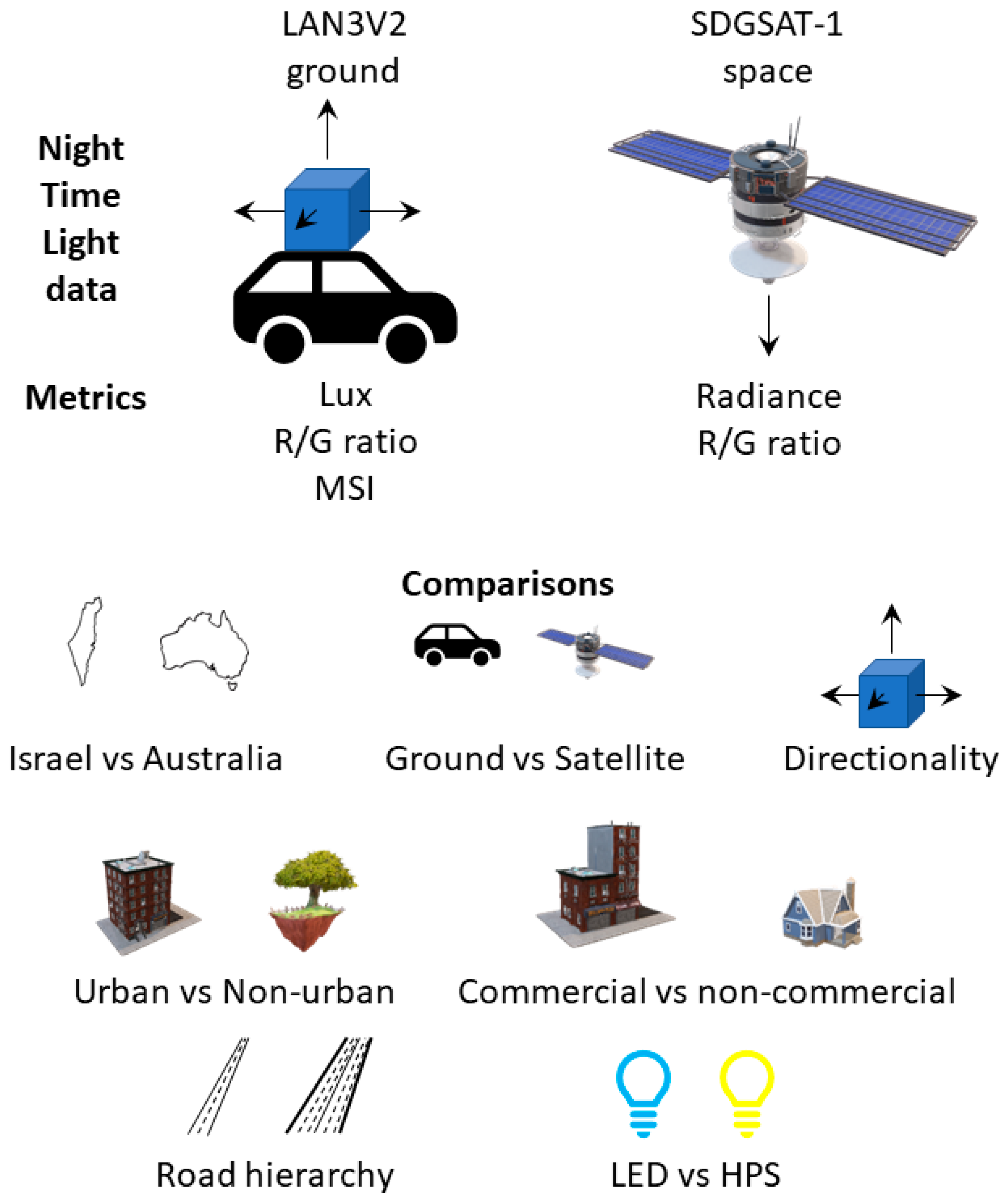
:1. Introduction
- To examine the differences in night-time lights as a function of road type and of urban land use.
- To examine the differences in the magnitude and color of night-time lights as measured in different directions, comparing roads in urban vs. rural areas.
- To examine whether measurements of night-time brightness in the horizontal direction improve our ability to explain night-time lights as measured from space.
- Highways belonging to a higher hierarchy would be more brightly lit than other road types and residential streets.
- Spaceborne measurements of night lights would be better explained by including ground based horizontal light emissions.
- The correlations between night-time brightness and color as measured in different directions will be low.
- The relative contribution of light from the different directions will vary as a function of the class of the road.
- In commercial areas, the contribution of horizontal light (as measured on the ground, especially to the left and right) to measured brightness will be greater than in residential areas.
- It will be easier to detect the type of street lighting from space outside of urban areas, given the multiple sources of artificial lights in urban areas. Therefore, we hypothesized that the variability in lighting, both in terms of its brightness and color using the metrics of the MSI (melatonin suppression index) and R/G ratio (red/green ratio) will be greater in urban road sections than in non-urban road sections.
2. Materials and Methods
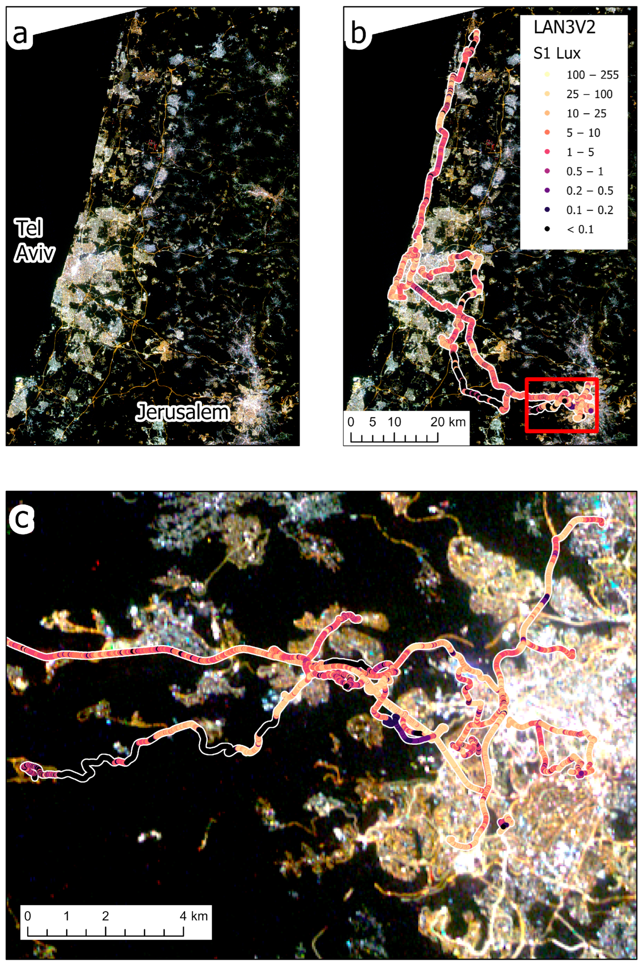
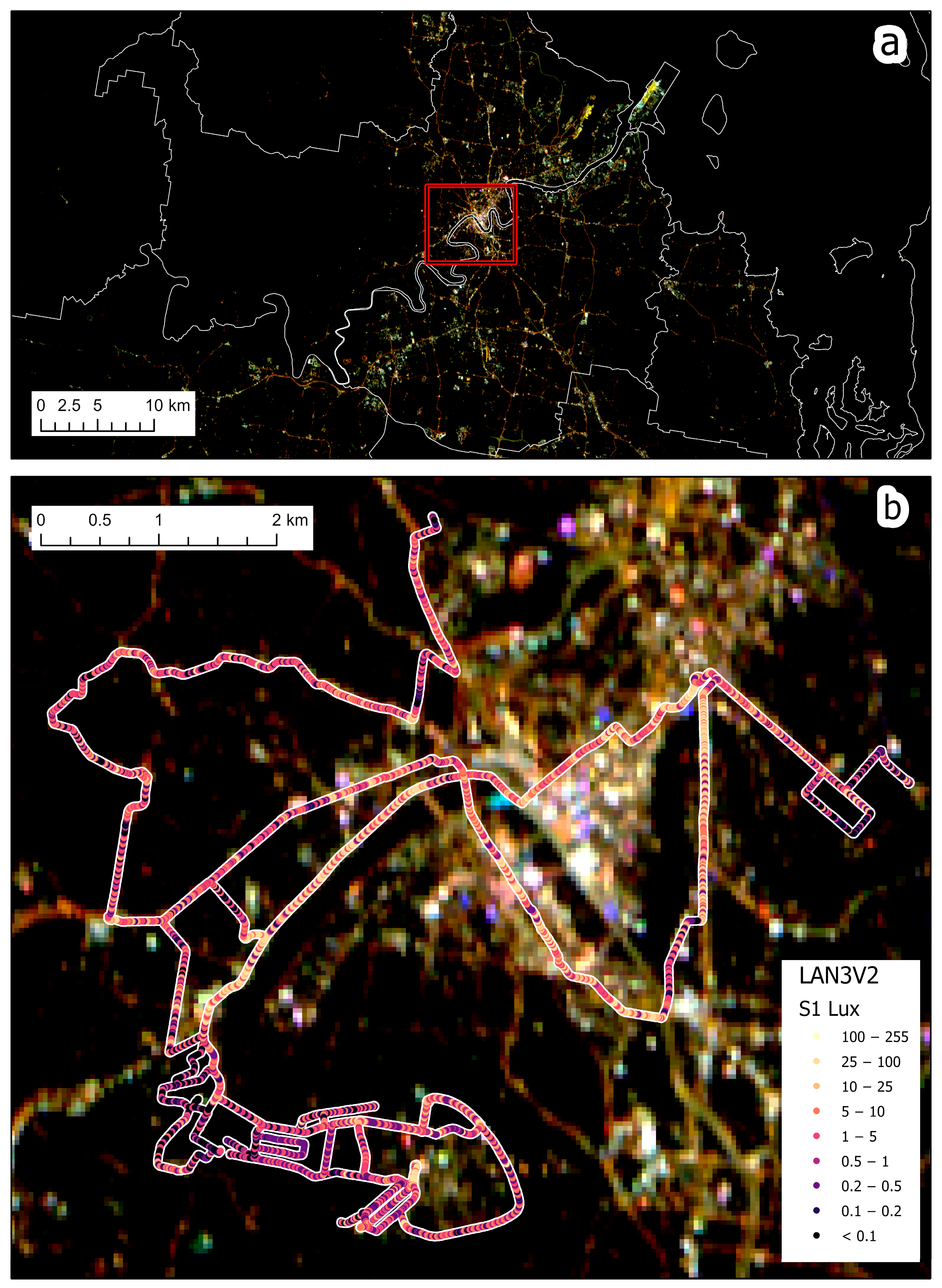
2.1. Study Area
2.2. Data Sets
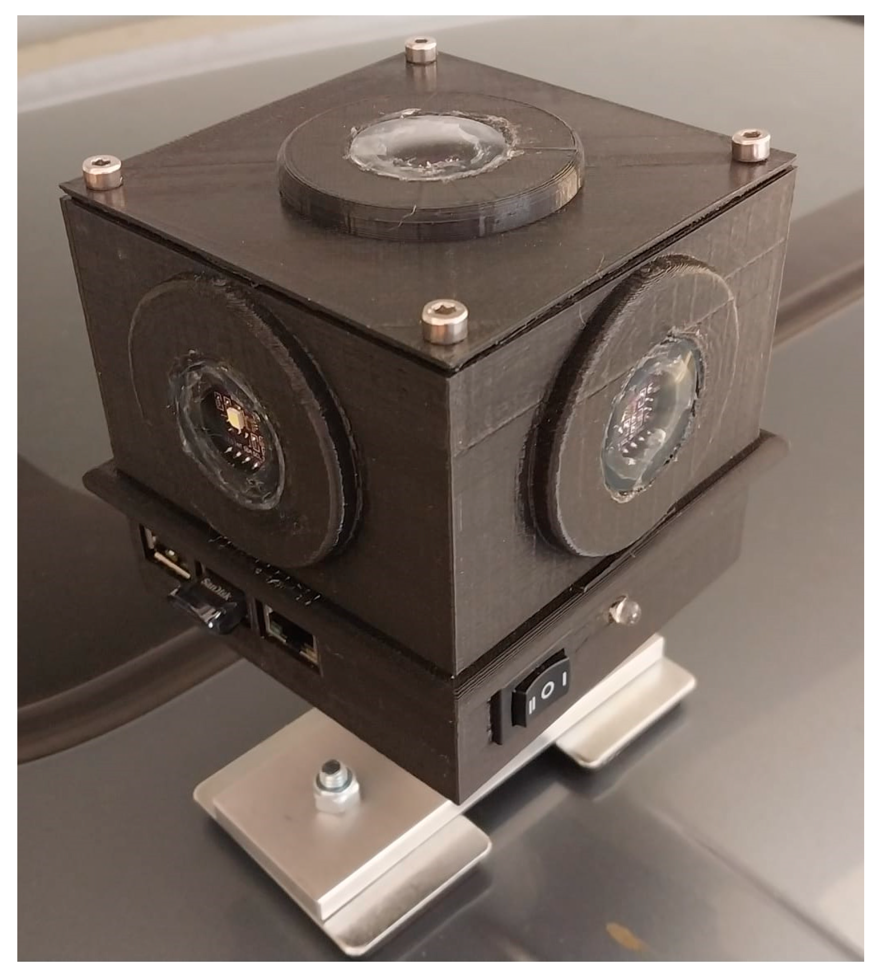
2.2.1. Ground Measurements
2.2.2. Space Borne Imagery
2.2.3. Supporting Datasets
2.3. Spatial and Statistical Analysis
3. Results
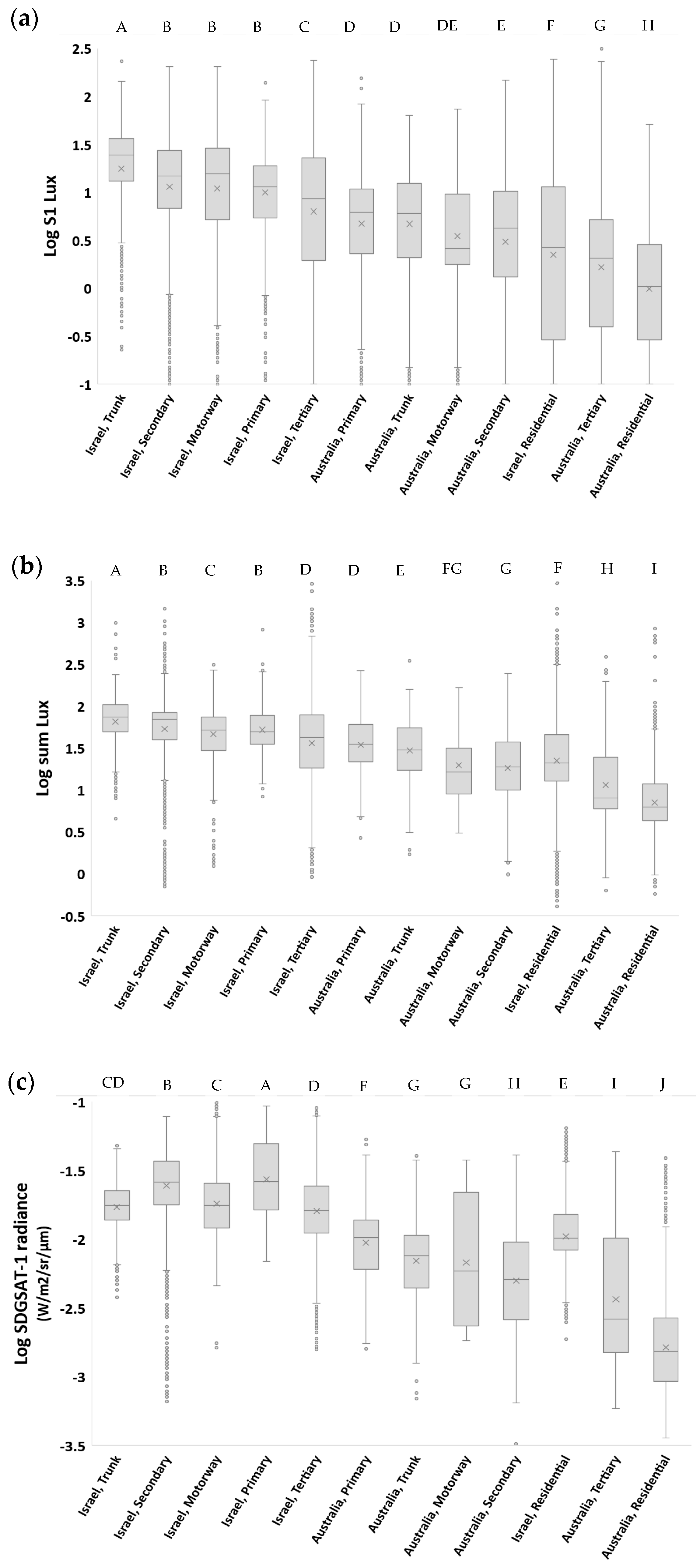
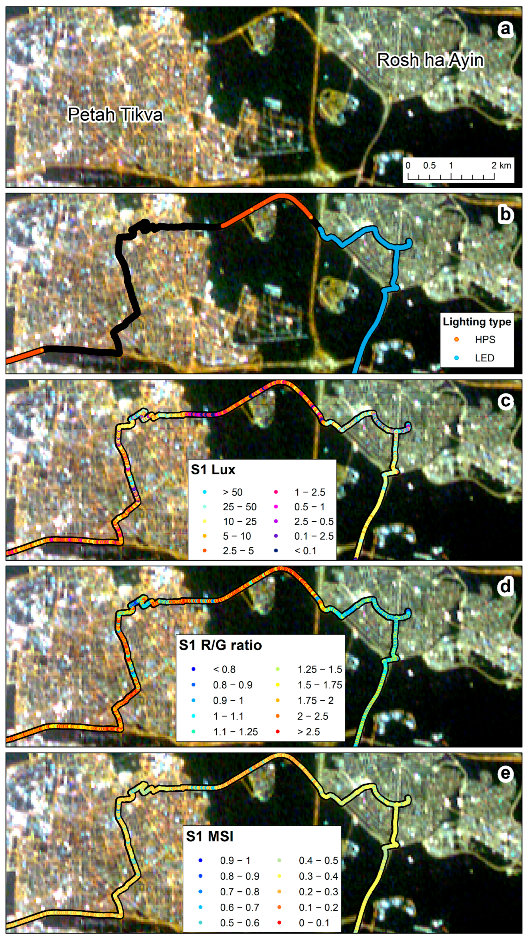
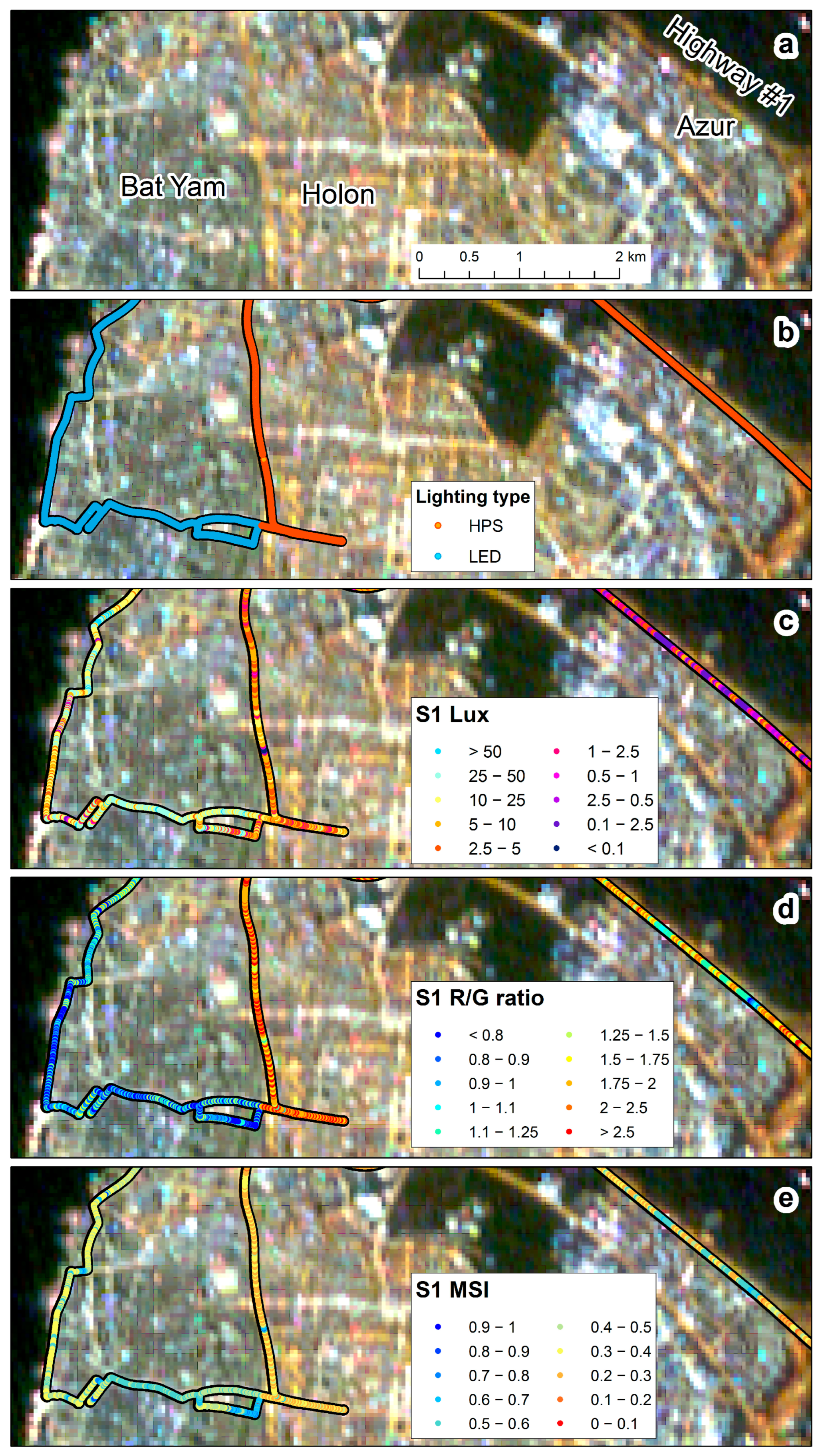
3.1. Comparisons between Road Classes and between Countries
3.2. Correlations between Ground-Based and Spaceborne Brightness Measurements
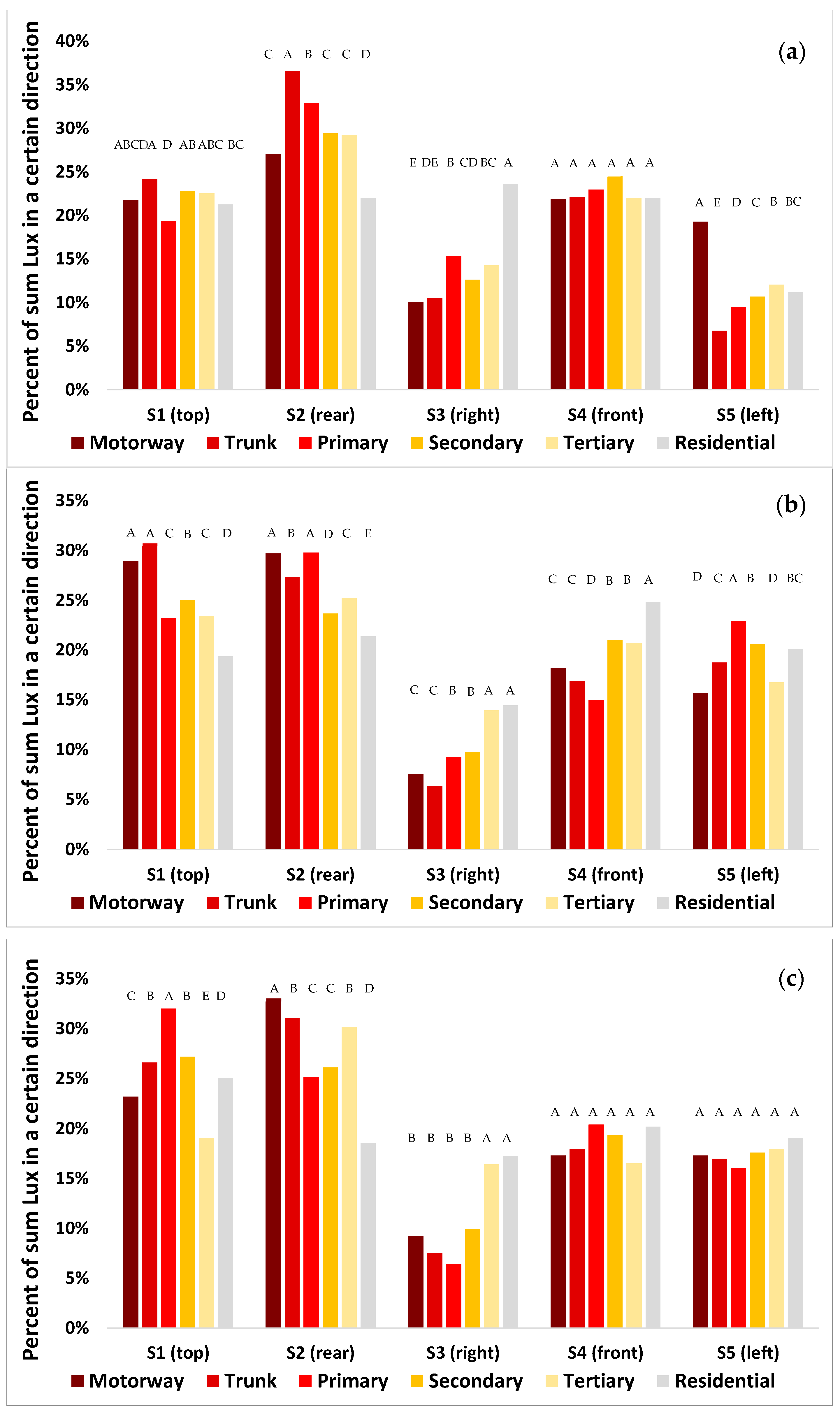
3.3. Comparisons between Ground Based Directional Measurements
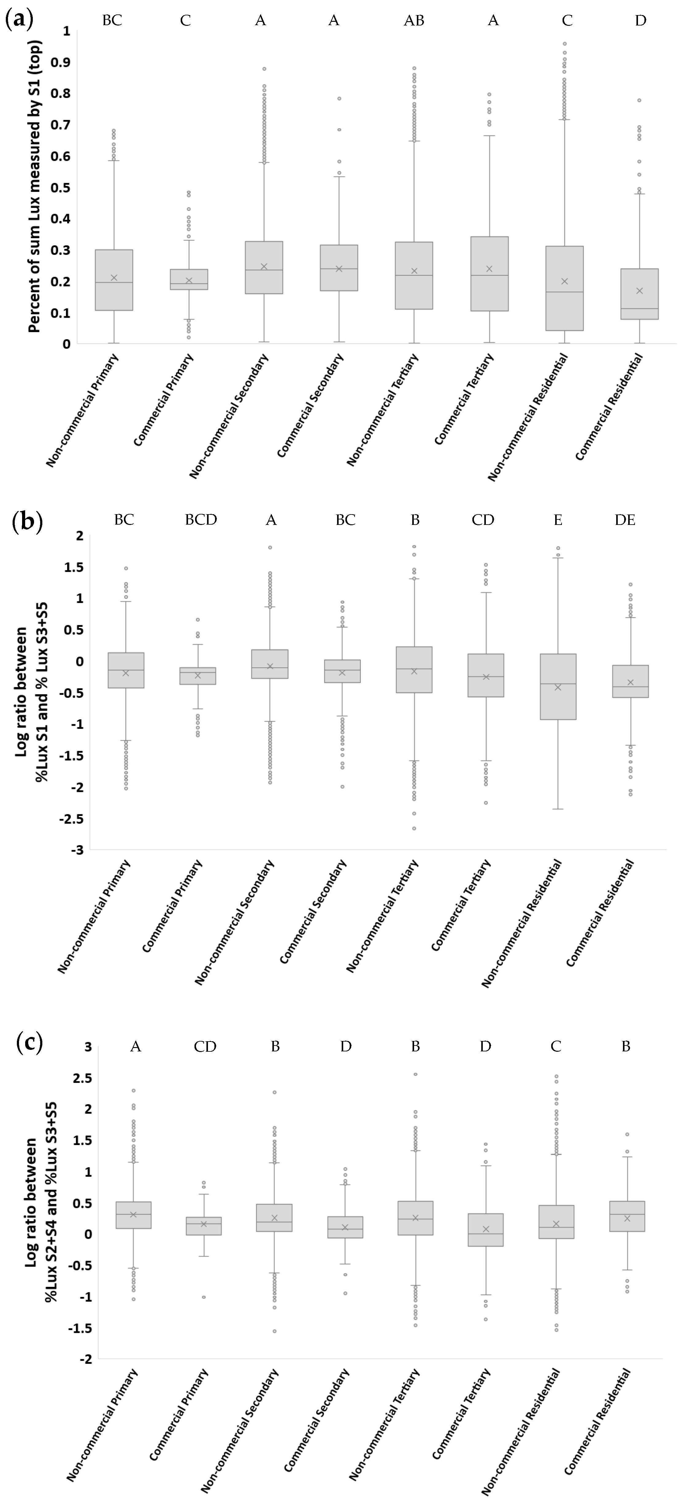
3.4. Comparisons between Commercial and Non-Commercial Locations
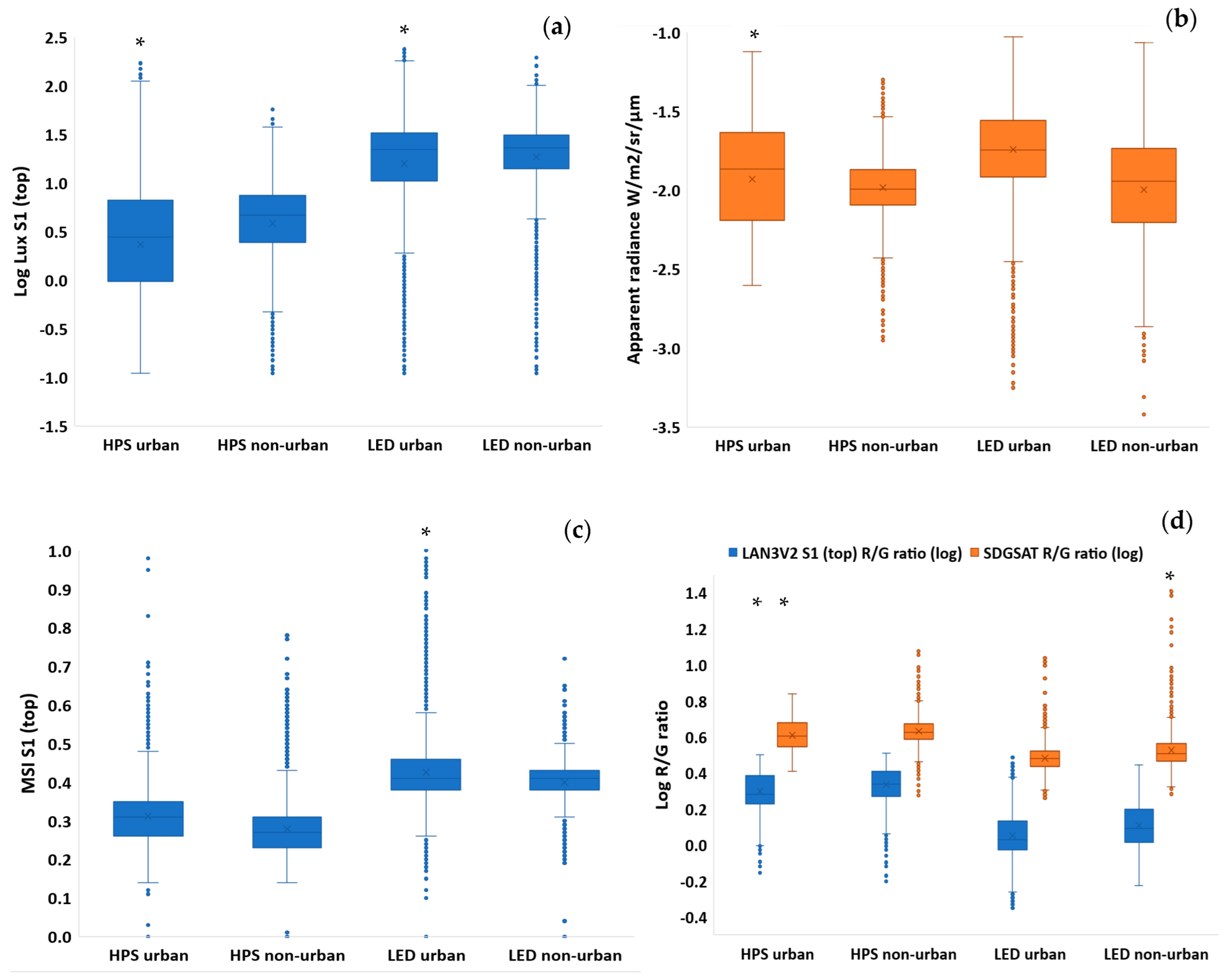
3.5. Comparisons between Urban and Non-Urban Road Sections
4. Discussion
5. Conclusions
Funding
Institutional Review Board Statement
Informed Consent Statement
Data Availability Statement
Acknowledgments
Conflicts of Interest
References
- Grimm, N.B.; Faeth, S.H.; Golubiewski, N.E.; Redman, C.L.; Wu, J.; Bai, X.; Briggs, J.M. Global Change and the Ecology of Cities. Science 2008, 319, 756–760. [Google Scholar] [CrossRef] [PubMed]
- Levin, N.; Kyba, C.C.M.; Zhang, Q.; Sánchez de Miguel, A.; Román, M.O.; Li, X.; Portnov, B.A.; Molthan, A.L.; Jechow, A.; Miller, S.D.; et al. Remote Sensing of Night Lights: A Review and an Outlook for the Future. Remote Sens. Environ. 2020, 237, 111443. [Google Scholar] [CrossRef]
- Kocifaj, M.; Wallner, S.; Barentine, J.C. Measuring and Monitoring Light Pollution: Current Approaches and Challenges. Science 2023, 380, 1121–1124. [Google Scholar] [CrossRef] [PubMed]
- Sánchez de Miguel, A.; Bennie, J.; Rosenfeld, E.; Dzurjak, S.; Gaston, K.J. First Estimation of Global Trends in Nocturnal Power Emissions Reveals Acceleration of Light Pollution. Remote Sens. 2021, 13, 3311. [Google Scholar] [CrossRef]
- Sánchez de Miguel, A.; Kyba, C.C.M.; Aubé, M.; Zamorano, J.; Cardiel, N.; Tapia, C.; Bennie, J.; Gaston, K.J. Colour Remote Sensing of the Impact of Artificial Light at Night (I): The Potential of the International Space Station and Other DSLR-Based Platforms. Remote Sens. Environ. 2019, 224, 92–103. [Google Scholar] [CrossRef]
- Zheng, Q.; Weng, Q.; Huang, L.; Wang, K.; Deng, J.; Jiang, R.; Ye, Z.; Gan, M. A New Source of Multi-Spectral High Spatial Resolution Night-Time Light Imagery—JL1-3B. Remote Sens. Environ. 2018, 215, 300–312. [Google Scholar] [CrossRef]
- Guo, B.; Hu, D.; Zheng, Q. Potentiality of SDGSAT-1 Glimmer Imagery to Investigate the Spatial Variability in Nighttime Lights. Int. J. Appl. Earth Obs. Geoinf. 2023, 119, 103313. [Google Scholar] [CrossRef]
- Tang, Y.; Dou, C.; Li, X.; Liu, J. SDGSAT-1 Data Users Handbook (Draft); International Research Center of Big Data for Sustainable Development Goals: Beijing, China, 2022. [Google Scholar]
- Elvidge, C.D.; Baugh, K.E.; Kihn, E.A.; Kroehl, H.W.; Davis, E.R.; Davis, C.W. Relation between Satellite Observed Visible-near Infrared Emissions, Population, Economic Activity and Electric Power Consumption. Int. J. Remote Sens. 1997, 18, 1373–1379. [Google Scholar] [CrossRef]
- Levin, N.; Zhang, Q. A Global Analysis of Factors Controlling VIIRS Nighttime Light Levels from Densely Populated Areas. Remote Sens. Environ. 2017, 190, 366–382. [Google Scholar] [CrossRef]
- Levin, N.; Duke, Y. High Spatial Resolution Night-Time Light Images for Demographic and Socio-Economic Studies. Remote Sens. Environ. 2012, 119, 1–10. [Google Scholar] [CrossRef]
- Kong, W.; Cheng, J.; Liu, X.; Zhang, F.; Fei, T. Incorporating Nocturnal UAV Side-View Images with VIIRS Data for Accurate Population Estimation: A Test at the Urban Administrative District Scale. Int. J. Remote Sens. 2019, 40, 8528–8546. [Google Scholar] [CrossRef]
- Guk, E.; Levin, N. Analyzing Spatial Variability in Night-Time Lights Using a High Spatial Resolution Color Jilin-1 Image—Jerusalem as a Case Study. ISPRS J. Photogramm. Remote Sens. 2020, 163, 121–136. [Google Scholar] [CrossRef]
- Li, X.; Ma, R.; Zhang, Q.; Li, D.; Liu, S.; He, T.; Zhao, L. Anisotropic Characteristic of Artificial Light at Night—Systematic Investigation with VIIRS DNB Multi-Temporal Observations. Remote Sens. Environ. 2019, 233, 111357. [Google Scholar] [CrossRef]
- Wang, Z.; Román, M.O.; Kalb, V.L.; Miller, S.D.; Zhang, J.; Shrestha, R.M. Quantifying Uncertainties in Nighttime Light Retrievals from Suomi-NPP and NOAA-20 VIIRS Day/Night Band Data. Remote Sens. Environ. 2021, 263, 112557. [Google Scholar] [CrossRef]
- Kyba, C.C.M.; Aubé, M.; Bará, S.; Bertolo, A.; Bouroussis, C.A.; Cavazzani, S.; Espey, B.R.; Falchi, F.; Gyuk, G.; Jechow, A.; et al. Multiple Angle Observations Would Benefit Visible Band Remote Sensing Using Night Lights. J. Geophys. Res. Atmos. 2022, 127, e2021JD036382. [Google Scholar] [CrossRef]
- Katz, Y.; Levin, N. Quantifying Urban Light Pollution—A Comparison between Field Measurements and EROS-B Imagery. Remote Sens. Environ. 2016, 177, 65–77. [Google Scholar] [CrossRef]
- Kyba, C.; Ruby, A.; Kuechly, H.; Kinzey, B.; Miller, N.; Sanders, J.; Barentine, J.; Kleinodt, R.; Espey, B. Direct Measurement of the Contribution of Street Lighting to Satellite Observations of Nighttime Light Emissions from Urban Areas. Light. Res. Technol. 2021, 53, 189–211. [Google Scholar] [CrossRef]
- Hänel, A.; Posch, T.; Ribas, S.J.; Aubé, M.; Duriscoe, D.; Jechow, A.; Kollath, Z.; Lolkema, D.E.; Moore, C.; Schmidt, N.; et al. Measuring Night Sky Brightness: Methods and Challenges. J. Quant. Spectrosc. Radiat. Transf. 2018, 205, 278–290. [Google Scholar] [CrossRef]
- Jechow, A.; Ribas, S.J.; Domingo, R.C.; Hölker, F.; Kolláth, Z.; Kyba, C.C.M. Tracking the Dynamics of Skyglow with Differential Photometry Using a Digital Camera with Fisheye Lens. J. Quant. Spectrosc. Radiat. Transf. 2018, 209, 212–223. [Google Scholar] [CrossRef]
- Kyba, C.C.M.; Ruhtz, T.; Fischer, J.; Hölker, F. Red Is the New Black: How the Colour of Urban Skyglow Varies with Cloud Cover: Red Is the New Black. Mon. Not. R. Astron. Soc. 2012, 425, 701–708. [Google Scholar] [CrossRef]
- Aubé, M.; Marseille, C.; Farkouh, A.; Dufour, A.; Simoneau, A.; Zamorano, J.; Roby, J.; Tapia, C. Mapping the Melatonin Suppression, Star Light and Induced Photosynthesis Indices with the LANcube. Remote Sens. 2020, 12, 3954. [Google Scholar] [CrossRef]
- Haklay, M. How Good Is Volunteered Geographical Information? A Comparative Study of OpenStreetMap and Ordnance Survey Datasets. Environ. Plan. B Plan. Des. 2010, 37, 682–703. [Google Scholar] [CrossRef]
- Reimann, C.; Filzmoser, P.; Garrett, R.G. Background and Threshold: Critical Comparison of Methods of Determination. Sci. Total Environ. 2005, 346, 1–16. [Google Scholar] [CrossRef] [PubMed]
- Verriotto, J.D.; Gonzalez, A.; Aguilar, M.C.; Parel, J.-M.A.; Feuer, W.J.; Smith, A.R.; Lam, B.L. New Methods for Quantification of Visual Photosensitivity Threshold and Symptoms. Trans. Vis. Sci. Technol. 2017, 6, 18. [Google Scholar] [CrossRef] [PubMed]
- Aube, M.; Houle, J.-P. Estimating Lighting Device Inventories with the LANcube v2 Multiangular Radiometer: Estimating Lighting Device Inventories. IJSL 2023, 25, 10–23. [Google Scholar] [CrossRef]
- Elvidge, C.D.; Cinzano, P.; Pettit, D.R.; Arvesen, J.; Sutton, P.; Small, C.; Nemani, R.; Longcore, T.; Rich, C.; Safran, J.; et al. The Nightsat Mission Concept. Int. J. Remote Sens. 2007, 28, 2645–2670. [Google Scholar] [CrossRef]
- Li, J.; Xu, Y.; Cui, W.; Ji, M.; Su, B.; Wu, Y.; Wang, J. Investigation of Nighttime Light Pollution in Nanjing, China by Mapping Illuminance from Field Observations and Luojia 1-01 Imagery. Sustainability 2020, 12, 681. [Google Scholar] [CrossRef]
- Li, X.; Shang, X.; Zhang, Q.; Li, D.; Chen, F.; Jia, M.; Wang, Y. Using Radiant Intensity to Characterize the Anisotropy of Satellite-Derived City Light at Night. Remote Sens. Environ. 2022, 271, 112920. [Google Scholar] [CrossRef]
- Xu, Y.; Knudby, A.; Côté-Lussier, C. Mapping Ambient Light at Night Using Field Observations and High-Resolution Remote Sensing Imagery for Studies of Urban Environments. Build. Environ. 2018, 145, 104–114. [Google Scholar] [CrossRef]
- Levin, N.; Johansen, K.; Hacker, J.M.; Phinn, S. A New Source for High Spatial Resolution Night Time Images—The EROS-B Commercial Satellite. Remote Sens. Environ. 2014, 149, 1–12. [Google Scholar] [CrossRef]
- Kuechly, H.U.; Kyba, C.C.M.; Ruhtz, T.; Lindemann, C.; Wolter, C.; Fischer, J.; Hölker, F. Aerial Survey and Spatial Analysis of Sources of Light Pollution in Berlin, Germany. Remote Sens. Environ. 2012, 126, 39–50. [Google Scholar] [CrossRef]
- Jie, N.; Cao, X.; Chen, J.; Chen, X. A New Method for Identifying the Central Business Districts with Nighttime Light Radiance and Angular Effects. Remote Sens. 2022, 15, 239. [Google Scholar] [CrossRef]
- Guo, Q.; Lin, M.; Meng, J.; Zhao, J. The Development of Urban Night Tourism Based on the Nightscape Lighting Projects--a Case Study of Guangzhou. Energy Procedia 2011, 5, 477–481. [Google Scholar] [CrossRef]
- Balasubramanian, S.; Irulappan, C.; Kitchley, J.L. Aesthetics of Urban Commercial Streets from the Perspective of Cognitive Memory and User Behavior in Urban Environments. Front. Archit. Res. 2022, 11, 949–962. [Google Scholar] [CrossRef]
- Brons, J.A.; Bullough, J.D.; Frering, D.C. Rational Basis for Light Emitting Diode Street Lighting Retrofit Luminaire Selection. Transp. Res. Rec. 2021, 2675, 634–638. [Google Scholar] [CrossRef]
- Watson, C.S.; Elliott, J.R.; Córdova, M.; Menoscal, J.; Bonilla-Bedoya, S. Evaluating Night-Time Light Sources and Correlation with Socio-Economic Development Using High-Resolution Multi-Spectral Jilin-1 Satellite Imagery of Quito, Ecuador. Int. J. Remote Sens. 2023, 44, 2691–2716. [Google Scholar] [CrossRef]
- Tabaka, P. Pilot Measurement of Illuminance in the Context of Light Pollution Performed with an Unmanned Aerial Vehicle. Remote Sens. 2020, 12, 2124. [Google Scholar] [CrossRef]
- Posch, T.; Binder, F.; Puschnig, J. Systematic Measurements of the Night Sky Brightness at 26 Locations in Eastern Austria. J. Quant. Spectrosc. Radiat. Transf. 2018, 211, 144–165. [Google Scholar] [CrossRef]
- Falchi, F.; Cinzano, P.; Duriscoe, D.; Kyba, C.C.M.; Elvidge, C.D.; Baugh, K.; Portnov, B.A.; Rybnikova, N.A.; Furgoni, R. The New World Atlas of Artificial Night Sky Brightness. Sci. Adv. 2016, 2, e1600377. [Google Scholar] [CrossRef]
- McCallum, I.; Kyba, C.C.M.; Bayas, J.C.L.; Moltchanova, E.; Cooper, M.; Cuaresma, J.C.; Pachauri, S.; See, L.; Danylo, O.; Moorthy, I.; et al. Estimating Global Economic Well-Being with Unlit Settlements. Nat. Commun. 2022, 13, 2459. [Google Scholar] [CrossRef]
- Kyba, C.C.M.; Kuester, T.; Sánchez de Miguel, A.; Baugh, K.; Jechow, A.; Hölker, F.; Bennie, J.; Elvidge, C.D.; Gaston, K.J.; Guanter, L. Artificially Lit Surface of Earth at Night Increasing in Radiance and Extent. Sci. Adv. 2017, 3, e1701528. [Google Scholar] [CrossRef] [PubMed]
- Sánchez de Miguel, A.; Bennie, J.; Rosenfeld, E.; Dzurjak, S.; Gaston, K.J. Environmental Risks from Artificial Nighttime Lighting Widespread and Increasing across Europe. Sci. Adv. 2022, 8, eabl6891. [Google Scholar] [CrossRef] [PubMed]


| Percent of All Measurements | ||||||
|---|---|---|---|---|---|---|
| Route Name | Date | Km | Unlit (Lux S1 < 0.1) | OSM Road Class | ||
| Motorway, Trunk, Primary | Secondary, Tertiary | Unclassified, Residential, Service | ||||
| Israel1 | 11 January 2022 | 3.3 | 15.3% | 0.0% | 11.6% | 88.4% |
| Israel2 | 12 January 2022 | 3.3 | 0.0% | 0.0% | 88.5% | 11.5% |
| Israel3 | 24 November 2022 | 19.8 | 2.4% | 18.7% | 57.9% | 23.4% |
| Israel4 | 3 December 2022 | 14.1 | 0.4% | 40.1% | 18.0% | 41.9% |
| Israel5 | 13 December 2022 | 127.0 | 6.7% | 67.1% | 16.6% | 16.3% |
| Israel6 | 18 December 2022 | 9.9 | 56.6% | 55.9% | 32.5% | 11.6% |
| Israel7 | 28 December 2022 | 33.2 | 25.1% | 26.3% | 59.2% | 14.5% |
| Israel8 | 2 January 2023 | 13.7 | 0.2% | 56.2% | 28.9% | 14.9% |
| Israel9 | 18 January 2023 | 12.2 | 9.6% | 21.0% | 54.1% | 24.9% |
| Israel10 | 20 January 2023 | 35.3 | 0.5% | 18.0% | 63.4% | 18.6% |
| Australia1 | 21 February 2023 | 13.5 | 10.2% | 0.0% | 30.8% | 69.2% |
| Australia2 | 21 March 2023 | 8.3 | 0.0% | 0.0% | 57.4% | 42.6% |
| Israel11 | 31 March 2023 | 4.6 | 0.0% | 0.0% | 75.8% | 24.2% |
| Israel12 | 14 April 2023 | 3.9 | 0.4% | 0.0% | 62.6% | 37.4% |
| Australia3 | 18 April 2023 | 26.2 | 10.2% | 32.4% | 47.4% | 20.2% |
| Australia4 | 23 April 2023 | 12.5 | 4.7% | 37.8% | 48.1% | 14.1% |
| Israel13 | 28 April 2023 | 11.2 | 0.1% | 63.2% | 30.3% | 6.5% |
| Israel14 | 12 May 2023 | 3.1 | 0.0% | 0.0% | 64.7% | 35.3% |
| Israel15 | 15 May 2023 | 103.1 | 15.5% | 51.6% | 29.9% | 18.6% |
| Total | 458.2 | 9.3% | 33.8% | 40.1% | 26.0% | |
| All Roads | Brisbane | Israel | Israel—Highways | Israel—Urban | ||
|---|---|---|---|---|---|---|
| Spearman rank correlation coefficients | S1 Lux (top) | 0.591 | 0.505 | 0.581 | 0.535 | 0.560 |
| S2 Lux (rear) | 0.608 | 0.629 | 0.601 | 0.519 | 0.614 | |
| S3 Lux (right) | 0.596 | 0.560 | 0.632 | 0.708 | 0.510 | |
| S4 Lux (front) | 0.596 | 0.605 | 0.592 | 0.503 | 0.581 | |
| S5 Lux (left) | 0.678 | 0.647 | 0.638 | 0.590 | 0.618 | |
| Sum Lux | 0.703 | 0.712 | 0.692 | 0.626 | 0.670 | |
| Linear regression Adjusted R2 | S1 Lux | 0.420 | 0.227 | 0.467 | 0.603 | 0.346 |
| Full model using all directional sensors | 0.625 | 0.526 | 0.644 | 0.725 | 0.556 | |
| n | 82,108 | 14,330 | 67,778 | 27,073 | 40,705 |
| HPS | LED | |||||||||
|---|---|---|---|---|---|---|---|---|---|---|
| S1 | S2 | S3 | S4 | S5 | S1 | S2 | S3 | S4 | S5 | |
| S1 | 0.40 | 0.37 | 0.36 | 0.23 | 0.30 | 0.51 | 0.48 | 0.20 | ||
| S2 | 0.61 | 0.32 | 0.22 | 0.28 | 0.30 | 0.39 | 0.24 | 0.16 | ||
| S3 | 0.42 | 0.43 | 0.20 | 0.20 | 0.34 | 0.26 | 0.29 | 0.23 | ||
| S4 | 0.52 | 0.37 | 0.49 | 0.24 | 0.31 | 0.22 | 0.23 | 0.21 | ||
| S5 | 0.65 | 0.56 | 0.33 | 0.50 | 0.29 | 0.24 | 0.17 | 0.21 | ||
| HPS | LED | |||||||||
|---|---|---|---|---|---|---|---|---|---|---|
| S1 | S2 | S3 | S4 | S5 | S1 | S2 | S3 | S4 | S5 | |
| S1 | 0.08 | 0.23 | 0.06 | 0.17 | 0.39 | 0.22 | 0.08 | 0.35 | ||
| S2 | 0.16 | 0.36 | 0.13 | 0.16 | 0.30 | 0.36 | 0.08 | 0.21 | ||
| S3 | 0.26 | 0.28 | 0.24 | 0.22 | 0.27 | 0.29 | 0.20 | 0.08 | ||
| S4 | 0.28 | 0.09 | 0.23 | 0.15 | 0.20 | 0.14 | 0.24 | 0.27 | ||
| S5 | 0.27 | 0.06 | 0.39 | 0.40 | 0.20 | 0.27 | 0.06 | 0.11 | ||
Disclaimer/Publisher’s Note: The statements, opinions and data contained in all publications are solely those of the individual author(s) and contributor(s) and not of MDPI and/or the editor(s). MDPI and/or the editor(s) disclaim responsibility for any injury to people or property resulting from any ideas, methods, instructions or products referred to in the content. |
© 2023 by the author. Licensee MDPI, Basel, Switzerland. This article is an open access article distributed under the terms and conditions of the Creative Commons Attribution (CC BY) license (https://creativecommons.org/licenses/by/4.0/).
Share and Cite
Levin, N. Quantifying the Variability of Ground Light Sources and Their Relationships with Spaceborne Observations of Night Lights Using Multidirectional and Multispectral Measurements. Sensors 2023, 23, 8237. https://doi.org/10.3390/s23198237
Levin N. Quantifying the Variability of Ground Light Sources and Their Relationships with Spaceborne Observations of Night Lights Using Multidirectional and Multispectral Measurements. Sensors. 2023; 23(19):8237. https://doi.org/10.3390/s23198237
Chicago/Turabian StyleLevin, Noam. 2023. "Quantifying the Variability of Ground Light Sources and Their Relationships with Spaceborne Observations of Night Lights Using Multidirectional and Multispectral Measurements" Sensors 23, no. 19: 8237. https://doi.org/10.3390/s23198237
APA StyleLevin, N. (2023). Quantifying the Variability of Ground Light Sources and Their Relationships with Spaceborne Observations of Night Lights Using Multidirectional and Multispectral Measurements. Sensors, 23(19), 8237. https://doi.org/10.3390/s23198237