
Extraction of Coastal Levees Using U-Net Model with Visible and Topographic Images Observed by High-Resolution Satellite Sensors


Abstract
1. Introduction
2. Materials and Methods
2.1. Proposed Method for Coastal Levee Extraction
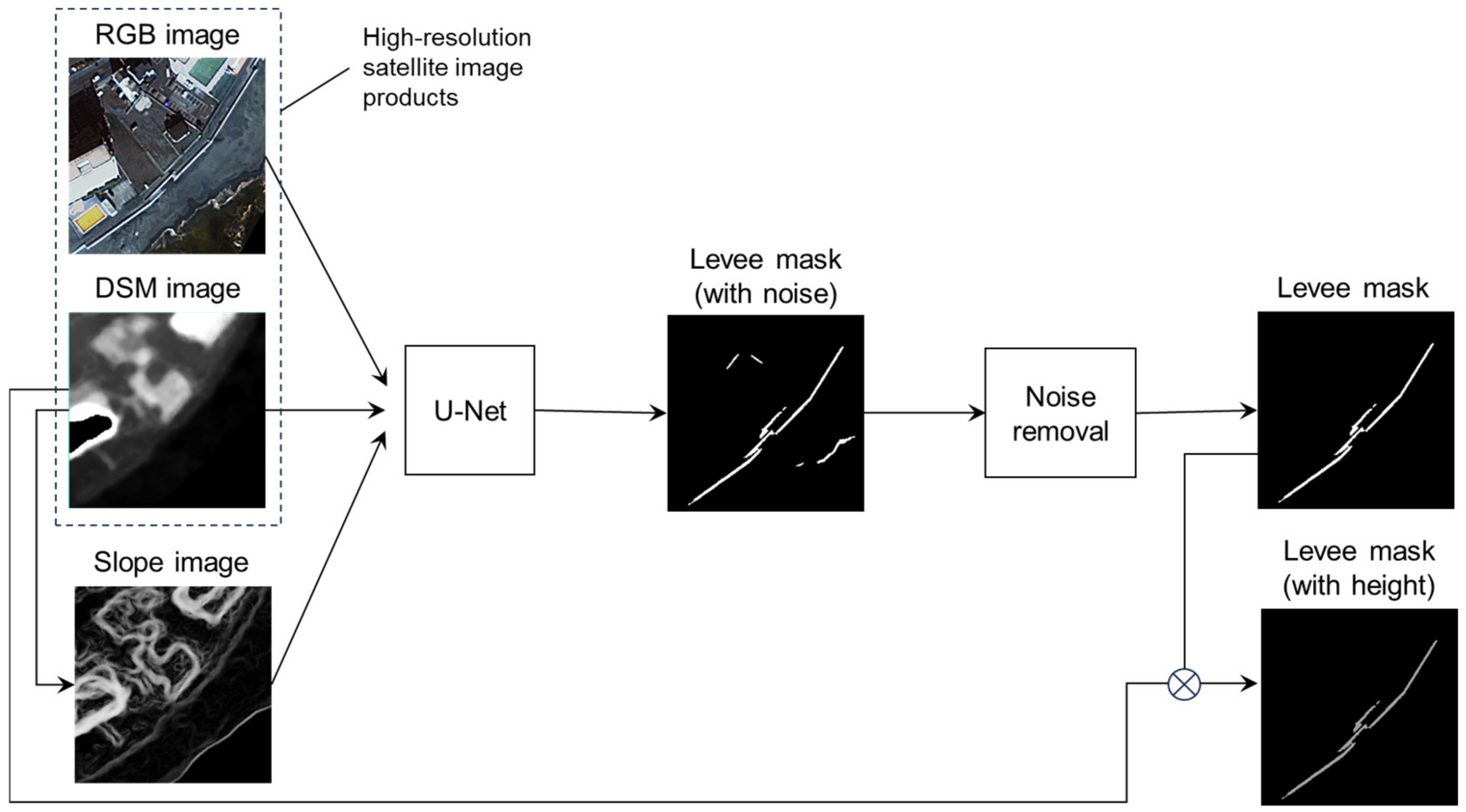
2.1.1. Method Overview
2.1.2. Structure and Parameters of the U-Net Model
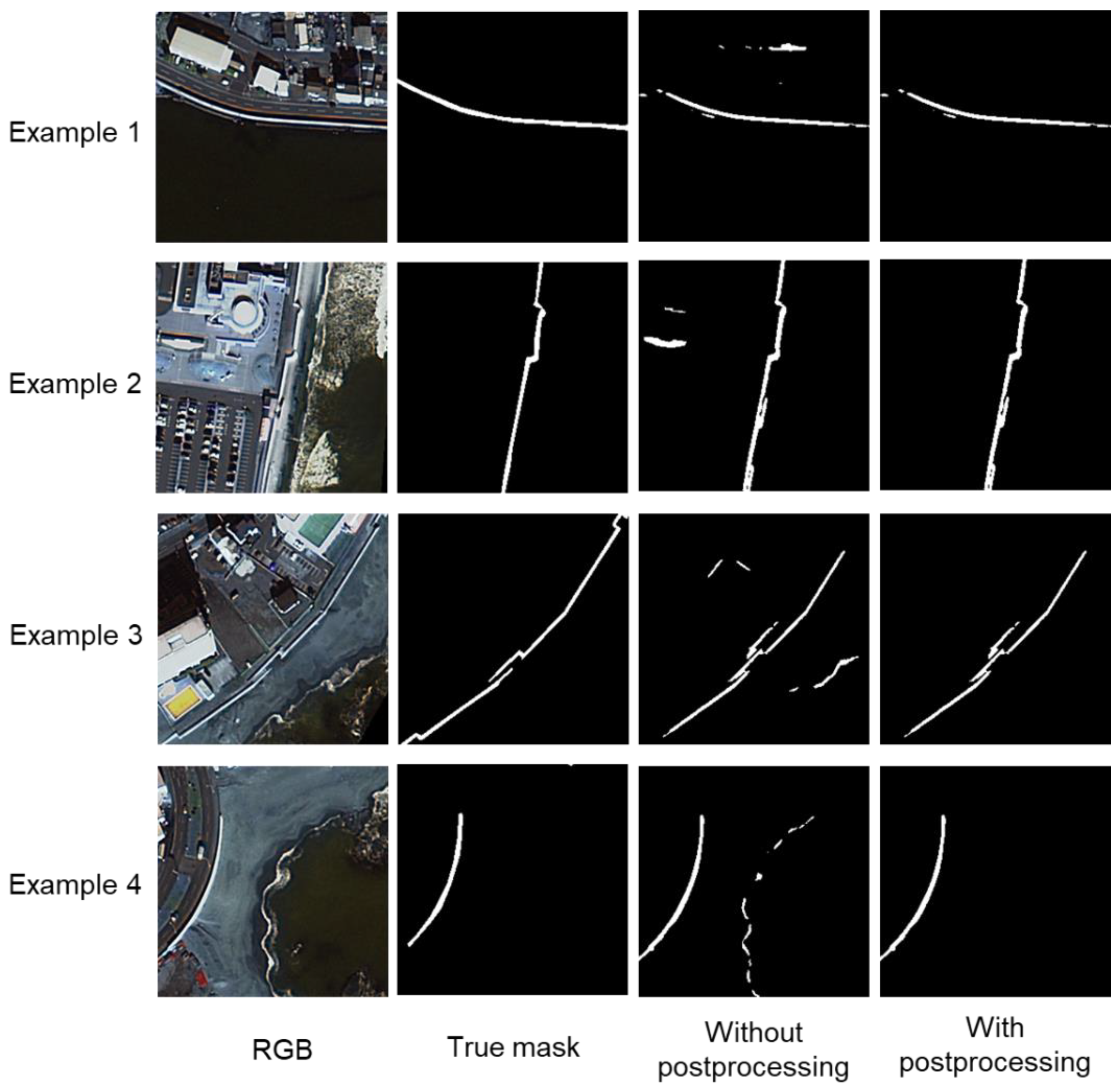
2.1.3. Post-Processing for Noise Removal
- Perform segmentation based on 8 connections for pixels extracted as levees.
- Select all segments within a predefined distance (20 pixels in this study) from the main segment with the highest number of pixels.
- Except for the main segment and the segments selected in (2), delete the remaining segments as noise.
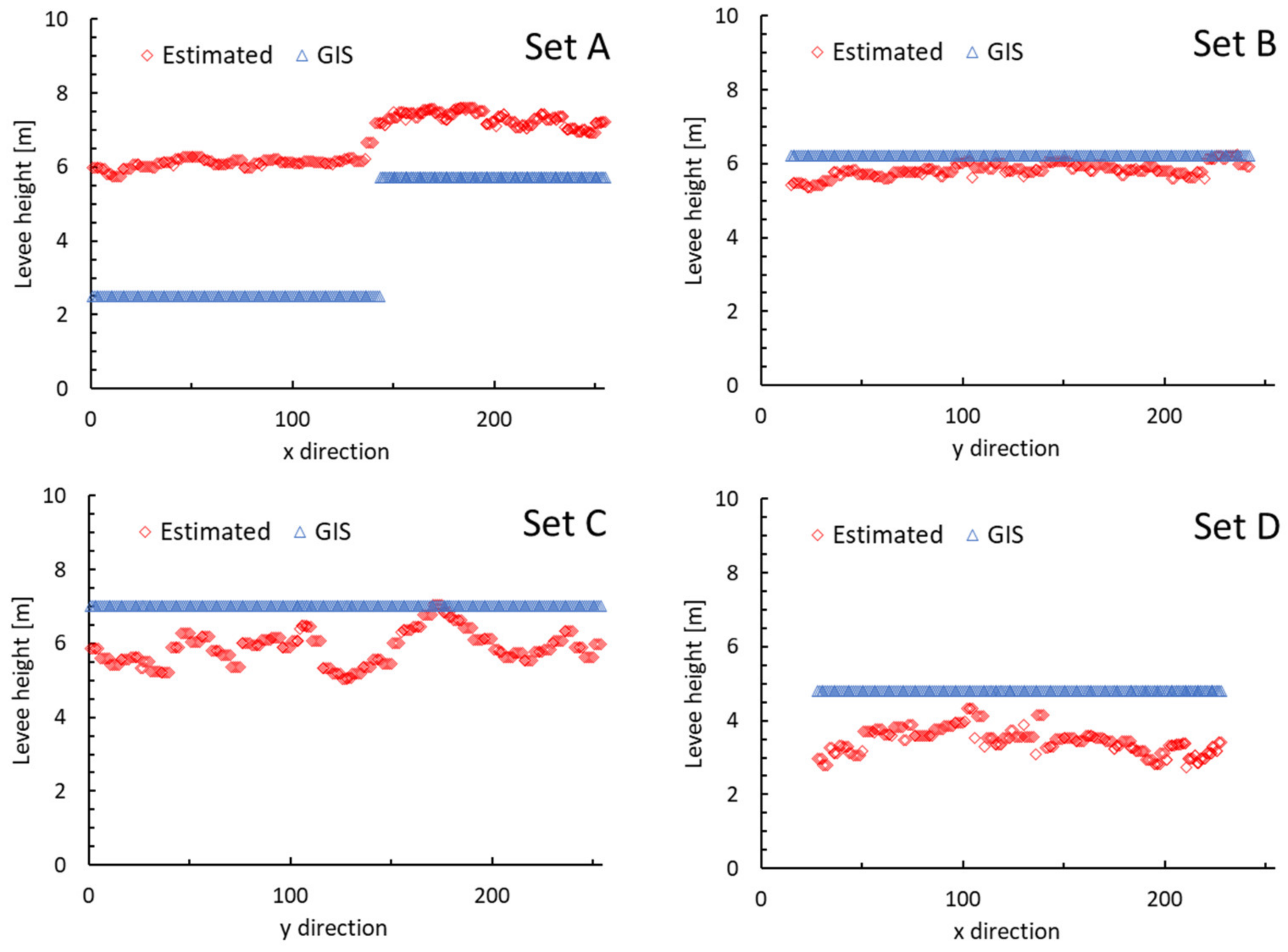
2.1.4. Calculation of Levee Height
2.2. Data Used
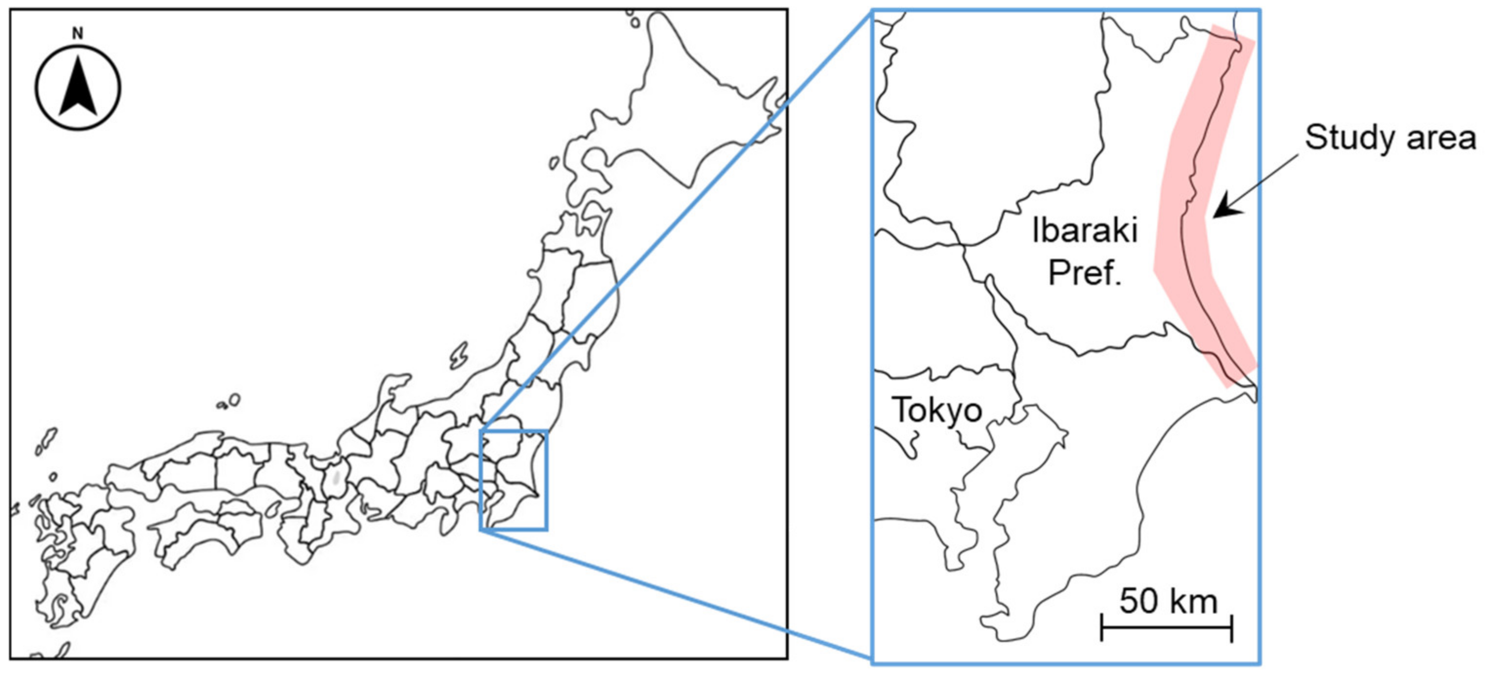
2.2.1. Study Area
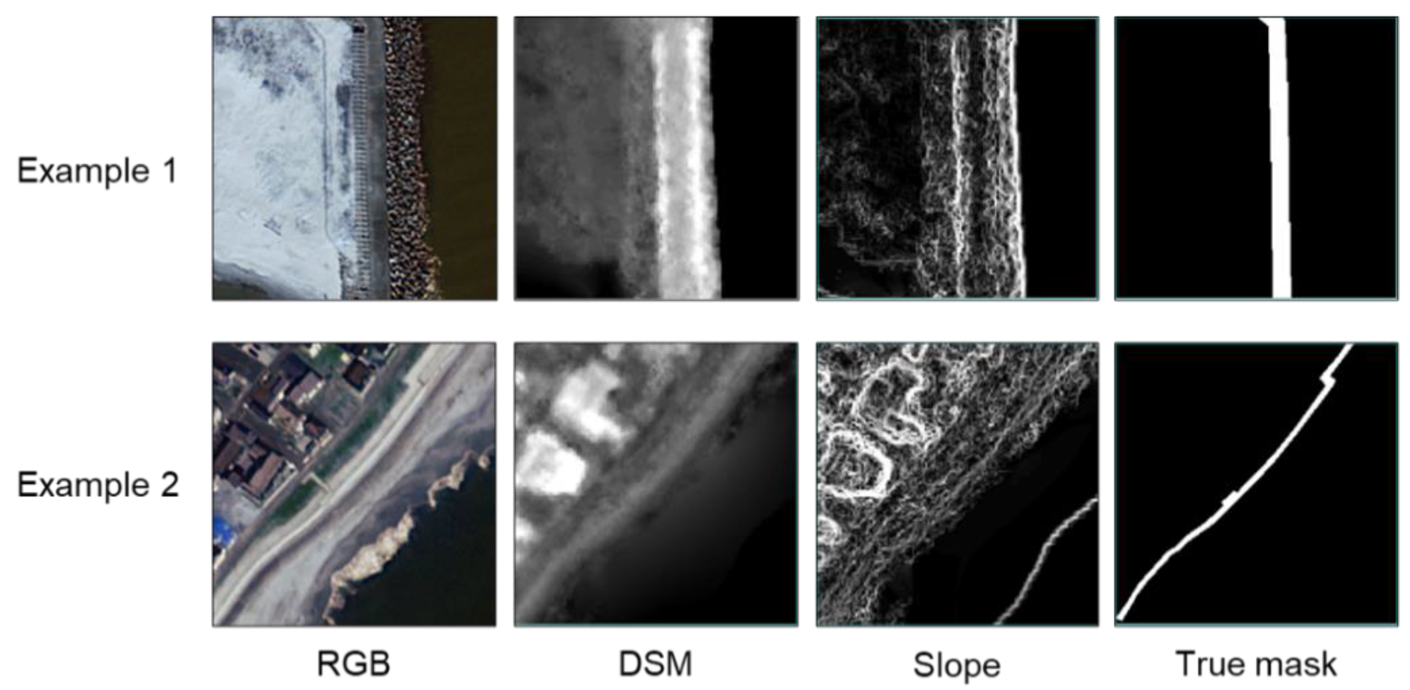
2.2.2. Input Images to U-Net
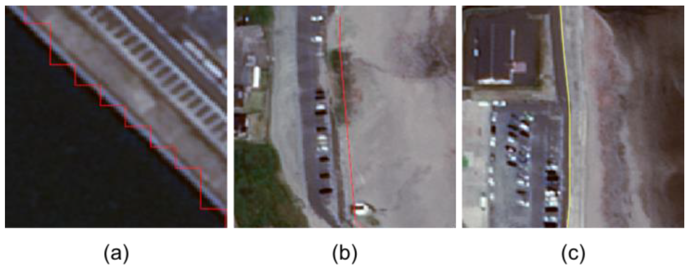
2.2.3. Levee Mask Images for Training
2.2.4. Subimage Sets
2.3. Learning and Evaluation
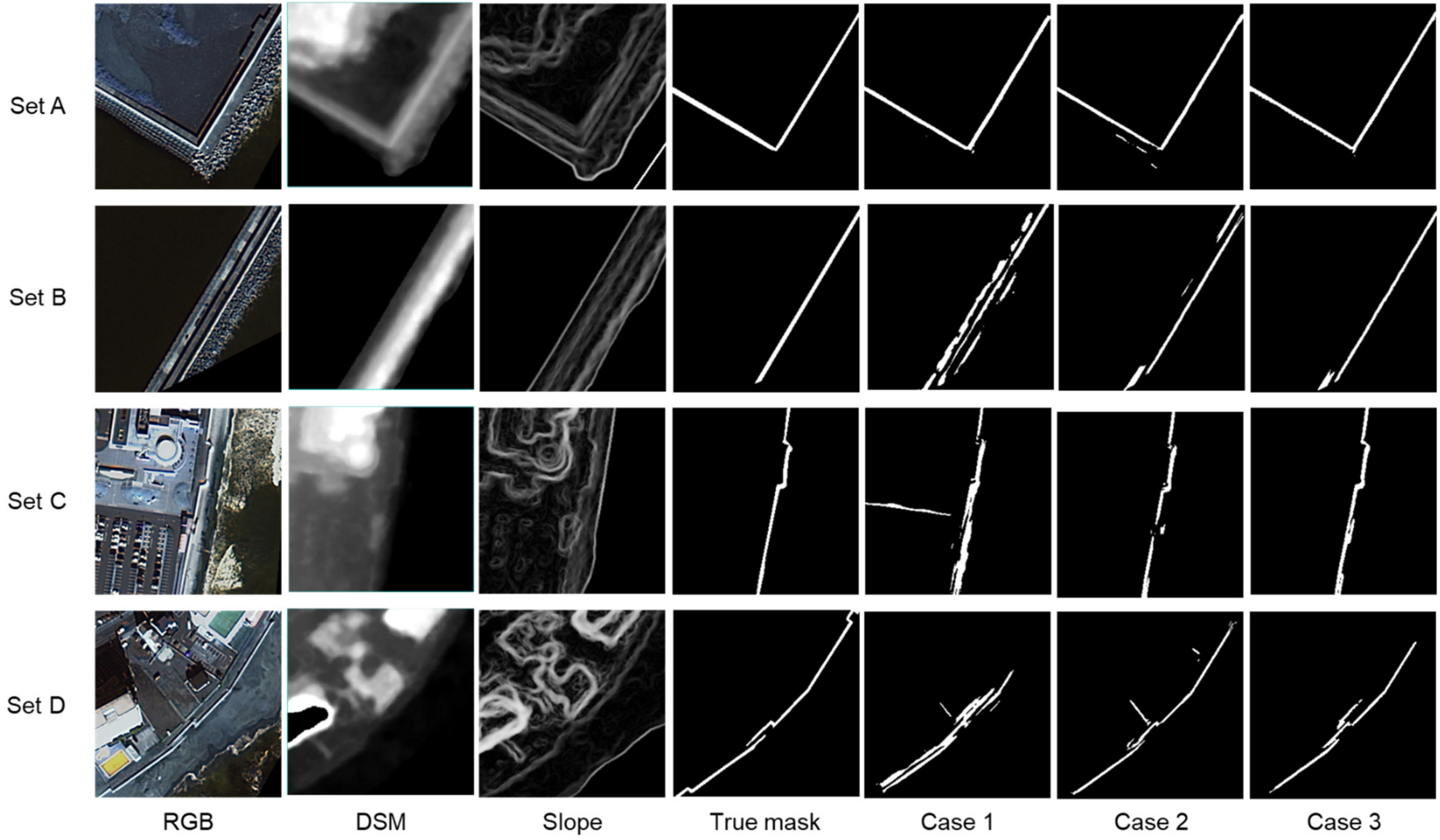
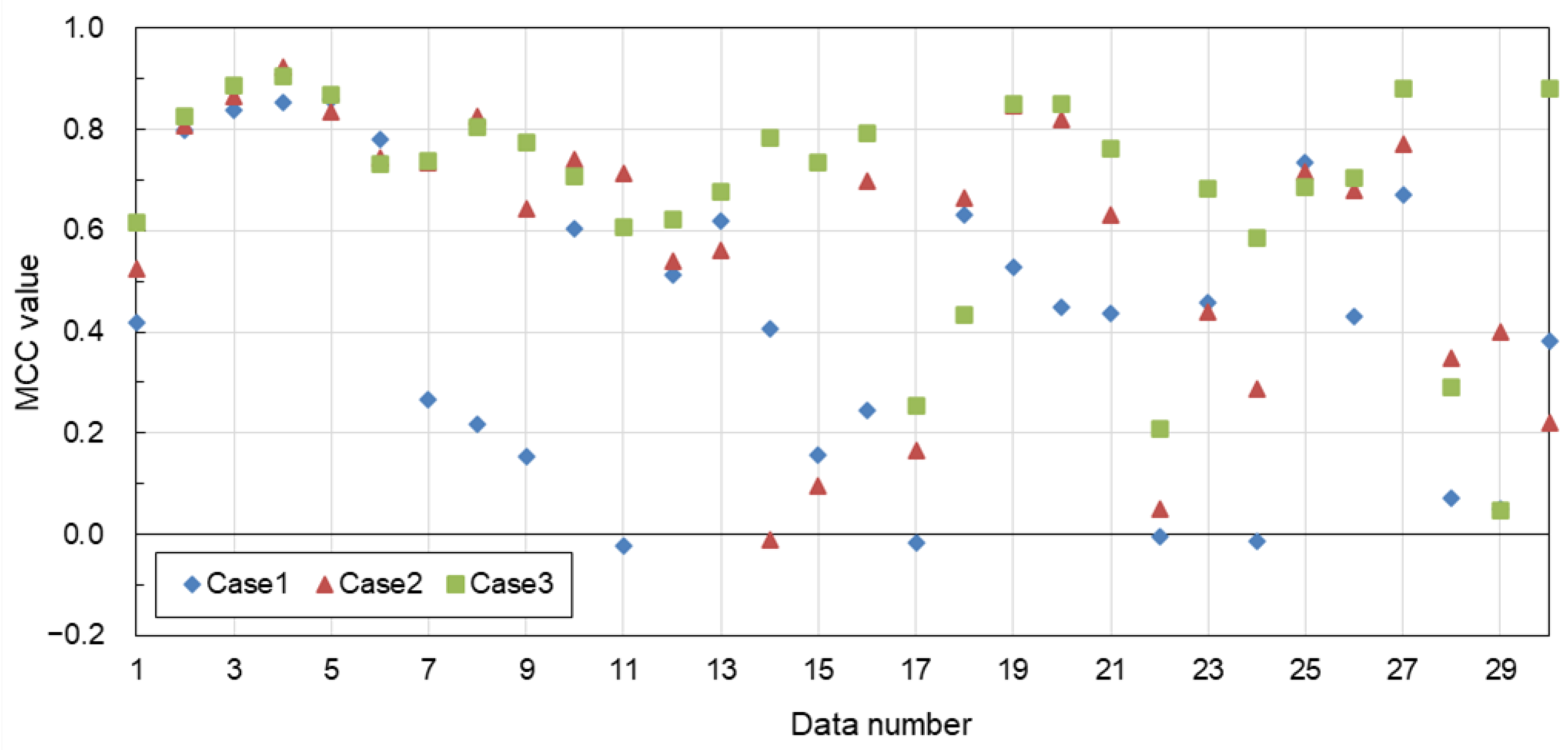
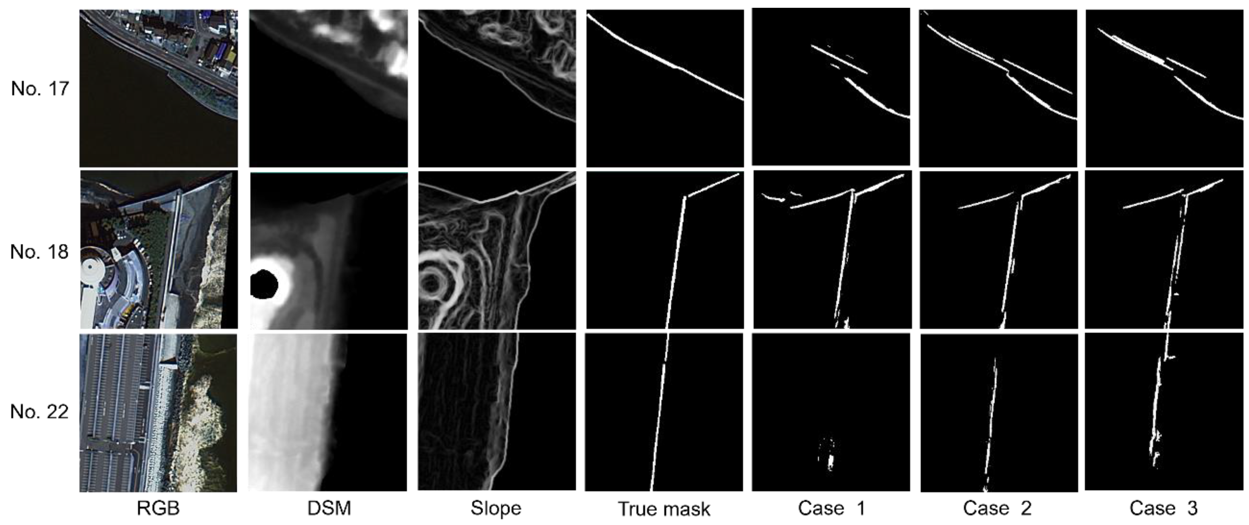
2.3.1. Evaluation Cases
- Case 1: Only RGB images were input;
- Case 2: RGB and DSM images were input;
- Case 3: RGB, DSM, and slope images were input.
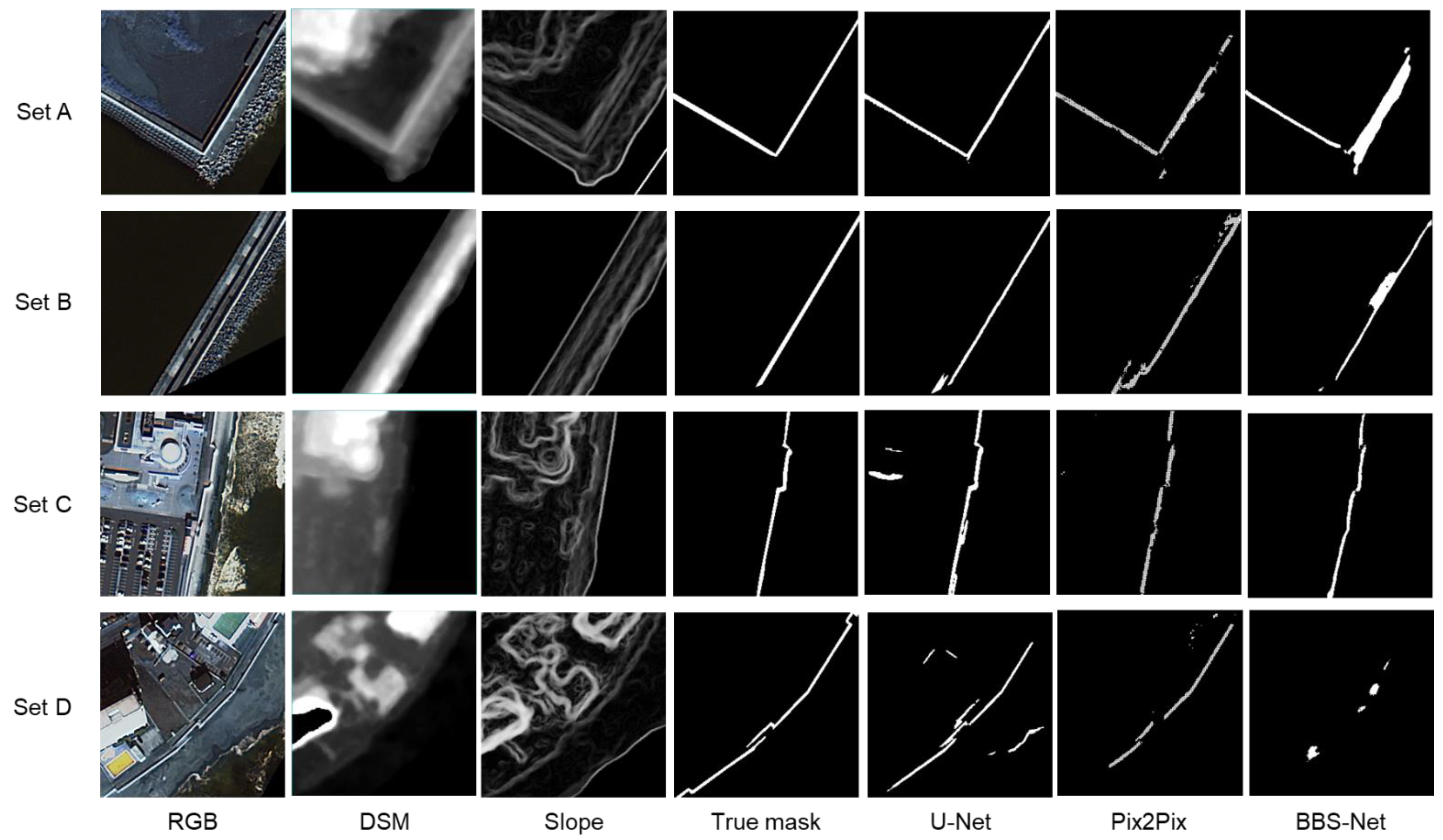
2.3.2. Deep Learning Models to Be Compared
2.3.3. Evaluation Indices
2.3.4. Evaluation of Levee Height
3. Results
4. Discussion
5. Conclusions
Author Contributions
Funding
Institutional Review Board Statement
Informed Consent Statement
Data Availability Statement
Acknowledgments
Conflicts of Interest
References
- Christensen, J.H.; Hewitson, B.; Busuioc, A.; Chen, A.; Gao, X.; Held, R.; Jones, R.; Kolli, R.K.; Kwon, W.K.; Laprise, R.; et al. Climate Change 2007: The Physical Science Basis: Contribution of Working Group I to the Fourth Assessment Report of the Intergovernmental Panel on Climate Change; Solomon, S., Intergovernmental Panel on Climate Change, Eds.; Cambridge University Press: Cambridge, UK; New York, NY, USA, 2007; ISBN 978-0-521-88009-1. [Google Scholar]
- Olbert, A.I.; Nash, S.; Cunnane, C.; Hartnett, M. Tide–Surge Interactions and Their Effects on Total Sea Levels in Irish Coastal Waters. Ocean. Dyn. 2013, 63, 599–614. [Google Scholar] [CrossRef]
- Von Storch, H.; Woth, K. Storm Surges: Perspectives and Options. Sustain. Sci. 2008, 3, 33–43. [Google Scholar] [CrossRef]
- Monirul Qader Mirza, M. Global Warming and Changes in the Probability of Occurrence of Floods in Bangladesh and Implications. Glob. Environ. Change. 2002, 12, 127–138. [Google Scholar] [CrossRef]
- Svetlana, D.; Radovan, D.; Ján, D. The Economic Impact of Floods and Their Importance in Different Regions of the World with Emphasis on Europe. Procedia Econ. Financ. 2015, 34, 649–655. [Google Scholar] [CrossRef]
- Grigorieva, E.; Livenets, A. Risks to the Health of Russian Population from Floods and Droughts in 2010–2020: A Scoping Review. Climate 2022, 10, 37. [Google Scholar] [CrossRef]
- Almar, R.; Ranasinghe, R.; Bergsma, E.W.J.; Diaz, H.; Melet, A.; Papa, F.; Vousdoukas, M.; Athanasiou, P.; Dada, O.; Almeida, L.P.; et al. A Global Analysis of Extreme Coastal Water Levels with Implications for Potential Coastal Overtopping. Nat. Commun. 2021, 12, 3775. [Google Scholar] [CrossRef]
- Chen, J.; Wang, Z.; Tam, C.-Y.; Lau, N.-C.; Lau, D.-S.D.; Mok, H.-Y. Impacts of Climate Change on Tropical Cyclones and Induced Storm Surges in the Pearl River Delta Region Using Pseudo-Global-Warming Method. Sci. Rep. 2020, 10, 1965. [Google Scholar] [CrossRef]
- Sahin, O.; Mohamed, S. Coastal Vulnerability to Sea-Level Rise: A Spatial–Temporal Assessment Framework. Nat. Hazards 2014, 70, 395–414. [Google Scholar] [CrossRef]
- Hallegatte, S.; Ranger, N.; Mestre, O.; Dumas, P.; Corfee-Morlot, J.; Herweijer, C.; Wood, R.M. Assessing climate change impacts, sea level rise and storm surge risk in port cities: A case study on Copenhagen. Clim. Chang. 2011, 104, 113–137. [Google Scholar] [CrossRef]
- Scussolini, P.; Aerts, J.C.J.H.; Jongman, B.; Bouwer, L.M.; Winsemius, H.C.; de Moel, H.; Ward, P.J. FLOPROS: An Evolving Global Database of Flood Protection Standards. Nat. Hazards Earth Syst. Sci. 2016, 16, 1049–1061. [Google Scholar] [CrossRef]
- Özer, I.E.; van Damme, M.; Jonkman, S.N. Towards an International Levee Performance Database (ILPD) and Its Use for Macro-Scale Analysis of Levee Breaches and Failures. Water 2020, 12, 119. [Google Scholar] [CrossRef]
- Steinfeld, C.M.M.; Kingsford, R.T.; Laffan, S.W. Semi-automated GIS Techniques for Detecting Floodplain Earthworks. Hydrol. Process. 2013, 27, 579–591. [Google Scholar] [CrossRef]
- Digital National Land Information Coastal Protection Facilities Data. Available online: https://nlftp.mlit.go.jp/ksj/gml/datalist/KsjTmplt-P23.html (accessed on 8 February 2024).
- Liu, Q.; Ruan, C.; Guo, J.; Li, J.; Lian, X.; Yin, Z.; Fu, D.; Zhong, S. Storm Surge Hazard Assessment of the Levee of a Rapidly Developing City-Based on LiDAR and Numerical Models. Remote Sens. 2020, 12, 3723. [Google Scholar] [CrossRef]
- Wing, O.E.J.; Bates, P.D.; Neal, J.C.; Sampson, C.C.; Smith, A.M.; Quinn, N.; Shustikova, I.; Domeneghetti, A.; Gilles, D.W.; Goska, R.; et al. A New Automated Method for Improved Flood Defense Representation in Large-Scale Hydraulic Models. Water Resour. Res. 2019, 55, 11007–11034. [Google Scholar] [CrossRef]
- Nienhuis, J.H.; Cox, J.R.; O’Dell, J.; Edmonds, D.A.; Scussolini, P. A Global Open-Source Database of Flood-Protection Levees on River Deltas (openDELvE). Nat. Hazards Earth Syst. Sci. 2022, 22, 4087–4101. [Google Scholar] [CrossRef]
- Ronneberger, O.; Fischer, P.; Brox, T. U-Net: Convolutional Networks for Biomedical Image Segmentation. In Medical Image Computing and Computer-Assisted Intervention—MICCAI 2015; Navab, N., Hornegger, J., Wells, W.M., Frangi, A.F., Eds.; Lecture Notes in Computer Science; Springer International Publishing: Cham, Switzerland, 2015; Volume 9351, pp. 234–241. ISBN 978-3-319-24573-7. [Google Scholar]
- Yan, C.; Fan, X.; Fan, J.; Wang, N. Improved U-Net Remote Sensing Classification Algorithm Based on Multi-Feature Fusion Perception. Remote Sens. 2022, 14, 1118. [Google Scholar] [CrossRef]
- Xu, Z.; Wang, S.; Stanislawski, L.V.; Jiang, Z.; Jaroenchai, N.; Sainju, A.M.; Shavers, E.; Usery, E.L.; Chen, L.; Li, Z.; et al. An Attention U-Net Model for Detection of Fine-Scale Hydrologic Streamlines. Environ. Model. Softw. 2021, 140, 104992. [Google Scholar] [CrossRef]
- Xu, W.; Deng, X.; Guo, S.; Chen, J.; Sun, L.; Zheng, X.; Xiong, Y.; Shen, Y.; Wang, X. High-Resolution U-Net: Preserving Image Details for Cultivated Land Extraction. Sensors 2020, 20, 4064. [Google Scholar] [CrossRef]
- Hormese, J.; Saravanan, C. Automated Road Extraction from High Resolution Satellite Images. Procedia Technol. 2016, 24, 1460–1467. [Google Scholar] [CrossRef]
- Hikosaka, S.; Tonooka, H. Image-to-Image Subpixel Registration Based on Template Matching of Road Network Extracted by Deep Learning. Remote Sens. 2022, 14, 5360. [Google Scholar] [CrossRef]
- Ovi, T.B.; Bashree, N.; Mukherjee, P.; Mosharrof, S.; Parthima, M.A. Performance Analysis of Various EfficientNet Based U-Net++ Architecture for Automatic Building Extraction from High Resolution Satellite Images. arXiv 2023, arXiv:2310.06847. [Google Scholar]
- Liu, W.; Yang, M.; Xie, M.; Guo, Z.; Li, E.; Zhang, L.; Pei, T.; Wang, D. Accurate Building Extraction from Fused DSM and UAV Images Using a Chain Fully Convolutional Neural Network. Remote Sens. 2019, 11, 2912. [Google Scholar] [CrossRef]
- Brown, C.; Smith, H.; Waller, S.; Weller, L.; Wood, D. Using image-based deep learning to identify river defenses from elevation data for large-scale flood modelling. In Proceedings of the EGU General Assembly 2020, Online, 4–8 May 2020. EGU2020-8522. [Google Scholar]
- Isola, P.; Zhu, J.Y.; Zhou, T.; Efros, A.A. Image-to-Image Translation with Conditional Adversarial Networks. arXiv 2016, arXiv:1611.07004. [Google Scholar]
- Zhai, Y.; Fan, D.-P.; Yang, J.; Borji, A.; Shao, L.; Han, J.; Wang, L. Bifurcated Backbone Strategy for RGB-D Salient Object Detection. IEEE Trans. Image Process. 2021, 30, 8727–8742. [Google Scholar] [CrossRef] [PubMed]
- Nitish, S.; Geoffrey, H.; Alex, K.; Ilya, S.; Ruslan, S. Dropout: A Simple Way to Prevent Neural Networks from Overfitting. Mach. Learn. Res. 2014, 15, 1929–1958. [Google Scholar]
- Liu, L.; Jiang, H.; He, P.; Chen, W.; Liu, X.; Gao, J.; Han, J. On the Variance of the Adaptive Learning Rate and Beyond. arXiv 2019, arXiv:1908.03265. [Google Scholar]
- Ibaraki Prefectural Living Environment. Available online: https://www.pref.ibaraki.jp/seikatsukankyo/bousaikiki/bousai/kirokushi/documents/shinsaikiroku-1syou.pdf (accessed on 8 January 2024).
- AW3D Ortho Imagery. Available online: https://www.aw3d.jp/products/ortho/ (accessed on 8 January 2024).
- AW3D Enhanced. Available online: https://www.aw3d.jp/products/enhanced/ (accessed on 8 January 2024).
- Pavlis, N.; Holmes, S.A.; Kenyon, S.; Factor, J. The development and evaluation of the Earth Gravitational Model 2008 (EGM2008). J. Geophys. Res. 2012, 117, B04406. [Google Scholar] [CrossRef]
- Matthews, B.W. Comparison of the Predicted and Observed Secondary Structure of T4 Phage Lysozyme. Biochim. Biophys. Acta (BBA) Protein Struct. 1975, 405, 442–451. [Google Scholar] [CrossRef]
- GIS Maps. Available online: https://maps.gsi.go.jp/ (accessed on 8 February 2024).

| Subarea Name | Satellite | Ground Resolution | Observation Date |
|---|---|---|---|
| Hazaki | GeoEye-1 | 0.5 m | 1 January 2023 |
| Kashima | WorldView-2 | 0.5 m | 10 May 2021 |
| Nakaminato and Oarai | WorldView-3 | 0.5 m | 19 December 2018 |
| Tokai | WorldView-2 | 0.5 m | 2 July 2022 |
| Kita-Ibaraki and Hitachi | WorldView-2/3 | 0.5 m | 21 April 2021, 5 August 2021, 25 November 2021 |
| Index | U-Net | Pix2Pix | BBS-Net |
|---|---|---|---|
| MCC | 0.648 | 0.521 | 0.533 |
| SSIM | 0.950 | 0.939 | 0.946 |
| IoU | 0.507 | 0.368 | 0.390 |
| Index | Case 1 (Only RGB) | Case 2 (RGB + DSM) | Case 3 (RGB + DSM + Slope) |
|---|---|---|---|
| MCC | 0.417 | 0.576 | 0.674 |
| SSIM | 0.926 | 0.951 | 0.958 |
| IoU | 0.309 | 0.447 | 0.542 |
| Index | Without Post-Processing | With Post-Processing |
|---|---|---|
| MCC | 0.648 | 0.674 |
| SSIM | 0.950 | 0.958 |
| IoU | 0.507 | 0.542 |
Disclaimer/Publisher’s Note: The statements, opinions and data contained in all publications are solely those of the individual author(s) and contributor(s) and not of MDPI and/or the editor(s). MDPI and/or the editor(s) disclaim responsibility for any injury to people or property resulting from any ideas, methods, instructions or products referred to in the content. |
© 2024 by the authors. Licensee MDPI, Basel, Switzerland. This article is an open access article distributed under the terms and conditions of the Creative Commons Attribution (CC BY) license (https://creativecommons.org/licenses/by/4.0/).
Share and Cite
Xia, H.; Tonooka, H. Extraction of Coastal Levees Using U-Net Model with Visible and Topographic Images Observed by High-Resolution Satellite Sensors. Sensors 2024, 24, 1444. https://doi.org/10.3390/s24051444
Xia H, Tonooka H. Extraction of Coastal Levees Using U-Net Model with Visible and Topographic Images Observed by High-Resolution Satellite Sensors. Sensors. 2024; 24(5):1444. https://doi.org/10.3390/s24051444
Chicago/Turabian StyleXia, Hao, and Hideyuki Tonooka. 2024. "Extraction of Coastal Levees Using U-Net Model with Visible and Topographic Images Observed by High-Resolution Satellite Sensors" Sensors 24, no. 5: 1444. https://doi.org/10.3390/s24051444
APA StyleXia, H., & Tonooka, H. (2024). Extraction of Coastal Levees Using U-Net Model with Visible and Topographic Images Observed by High-Resolution Satellite Sensors. Sensors, 24(5), 1444. https://doi.org/10.3390/s24051444